Geological–Engineering Synergistic Optimization of CO₂ Flooding Well Patterns for Sweet Spot Development in Tight Oil Reservoirs

Abstract

CO₂ flooding technology has been established as a key technique that is both economically viable and environmentally sustainable, achieving enhanced oil recovery (EOR) while advancing CCUS objectives. This study addresses the challenge of optimizing CO₂ flooding well patterns in tight oil reservoirs through a geological–engineering integrated approach. A semi-analytical model incorporating startup pressure gradients and miscible/immiscible two-phase flow was developed to dynamically adjust injection intensity. An effective driving coefficient model considering reservoir heterogeneity and fracture orientation was proposed to determine well pattern boundaries. Field data from Blocks A and B were used to validate the models, with the results indicating optimal injection intensities of 0.39 t/d/m and 0.63 t/d/m, respectively. Numerical simulations confirmed that inverted five-spot patterns with well spacings of 240 m (Block A) and 260 m (Block B) achieved the highest incremental oil production (3621.6 t/well and 4213.1 t/well) while reducing the gas channeling risk by 35–47%. The proposed methodology provides a robust framework for enhancing recovery efficiency in low-permeability reservoirs under varying geological conditions.

1. Introduction

As a major greenhouse gas, the environmental impact caused by excessive emissions of CO₂ has become the focus of global attention [1,2,3,4,5], resulting in adverse effects such as increased climate warming, ocean acidification [6,7,8] and ecosystem disturbance [9]. Underground sequestration of CO₂ is an important way to reduce carbon emissions and convert greenhouse gases into tools for improving energy efficiency [10,11,12,13,14], while achieving the unity of environmental and economic benefits [15,16,17]. The geo-engineering collaborative optimization method of this study further improves the utilization efficiency of CO₂ in complex reservoirs, integrates CO₂ storage with enhanced oil recovery, and provides a reproducible low-carbon solution for the development of low permeability reservoirs around the world, promoting the long-term development of carbon neutrality.

In recent years, due to the continuous growth of global energy demand, the exploration and development of tight oil reservoirs have become increasingly important [18,19]. Tight oil is characterized by extremely low permeability and porosity [20,21], posing significant challenges to efficient production. Conventional production methods often lead to a rapid decline in formation energy and low recovery rates. To address these issues, enhanced oil recovery (EOR) techniques, particularly carbon dioxide (CO₂) injection, have emerged as a promising solution [22,23,24,25,26].

CO₂ injection in tight oil reservoirs not only helps maintain reservoir pressure but also improves displacement efficiency through miscible or near-miscible interactions with crude oil [27,28]. However, the success of CO₂ injection in tight oil reservoirs largely depends on well pattern design and injection parameters [29]. Determining the optimal well pattern limits and injection strategies is crucial for maximizing sweep efficiency and ultimately enhancing crude oil recovery.

Previous studies have made significant contributions to understanding reservoir seepage mechanisms and optimizing well pattern development schemes. For example, Zhu, W. et al. [30], combined with the theory of elliptical seepage in fracturing, proposed a calculation method for the utilization coefficient under different well pattern fracturing conditions, providing a theoretical basis for reservoir evaluation and development design in low-permeability reservoirs. Chi, J. et al. established a mathematical model for simultaneous CO₂ miscible and immiscible flooding that accounts for oil viscosity changes and threshold pressure gradients of oil–gas and CO₂ based on non-Darcy seepage theory [31]. Subsequently, the team further focused on the CO₂ immiscible flooding scenario, developing a corresponding mathematical model through in-depth research to provide a robust theoretical tool for exploring CO₂ flooding mechanisms and optimizing production schemes [32]. Zhang, N. et al. proposed key parameters for CO₂ miscible flooding guidelines to facilitate carbon capture and storage [33]. Sun, H. et al. introduced a hybrid model linking pore-scale and continuum-scale computations to observe phenomena unaccounted for by Darcy-scale models in porous media flow and transport. Sun H developed a two-phase seepage–stress coupling formulation based on Co-NMM, considering complex multi-fracture propagation and matrix–fracture interface effects on two-phase flow in fractured porous media [34].

However, few studies have been reported based on non-Darcy percolation theory, combined with starting pressure gradient and miscibility/immiscibility two-phase flow dynamics, and considering both fracture and reservoir heterogeneity.

To address these gaps, this study constructs a semi-analytical model coupling startup pressure gradients and CO₂ miscible/immiscible two-phase flow under non-Darcy seepage theory. A three-region seepage model is established to dynamically adjust injection intensity. An effective driving coefficient model considering reservoir heterogeneity and fracture orientation is proposed to determine well pattern lower limits, validated via CMG numerical simulation. The research aims to achieve bidirectional optimization of efficient CO₂ storage and enhanced oil recovery, providing theoretical support for low-permeability reservoir development under the “double carbon” goal.

These advancements enable the precise determination of well pattern boundaries and injection parameters, providing a theoretical foundation for CO₂ flooding in tight reservoirs that differs from previous homogeneous models. The results show that the reverse five-point pattern has a better development effect on CO₂ flooding in tight reservoirs.

2. Establishment of Injection and Production Theoretical Model

Well pattern type is a critical consideration in CO₂ flooding reservoir engineering design. Based on the stress-sensitive-seepage coupling development concept proposed by Li et al. [35], well pattern optimization requires an integrated analysis of fracture characteristics and in situ stress field distribution to achieve efficient displacement through optimized well row orientation and injection-production parameters. Studies demonstrate that aligning injector rows with the maximum principal stress direction creates preferential linear flow paths, enabling uniform CO₂ diffusion within fractured networks and effectively mitigating gas channeling risks [36]. This deployment strategy controls the gas–liquid interface propagation velocity within 0.3–0.5 m/d through injection-production pressure differential management, increasing sweep volume coefficients to 68–72% [37].

In low-permeability reservoirs undergoing CO₂ miscible flooding, crude oil property alterations caused by dissolution effects introduce dynamic seepage resistance changes that complicate flow mechanisms compared to waterflooding. A variable well spacing calculation method for CO₂ flooding was developed by integrating displacement characteristics and flow patterns. Reservoirs are divided into miscible and immiscible zones from injectors to producers, and the technical limit well spacing formula for CO₂ flooding was derived using Darcy’s law [36].

Field applications globally confirm the adaptability of five-spot patterns in low-permeability reservoirs. The Sundown Slaughter Unit in the U.S. achieved 35% better gas channeling control with linear displacement patterns (200–300 m spacing) compared to earlier herringbone patterns in heterogeneous reservoirs [38]. Canada’s Weyburn Field employed a hybrid horizontal injector–vertical producer well system combined with CO₂–water alternating gas (WAG) injection to achieve stable daily oil increments of 1.8–2.3 t per well in reservoirs with vertical permeability variation coefficients of 0.85 [36].

In the Gao 89-Fan 142 area of Shengli Oilfield, CO₂ flooding demonstration projects using the technical limit well spacing model determined optimal spacing ranges of 350–510 m (average 405 m). As of March 2024, no major gas channeling had occurred, with nearly half of the wells showing significant production improvements. Existing well spacings in the area are below technical limits, making them suitable for CO₂ flooding. For blocks with smaller spacings, WAG injection is recommended to control channeling, with potential injection-production adjustments for channeling well groups during late-stage development.

This section study innovatively introduces:

• A semi-analytical model incorporating startup pressure gradients and miscible/immiscible two-phase flow to dynamically adjust injection intensity.
• An effective driving coefficient model that quantifies well pattern efficiency considering reservoir heterogeneity.

2.1. Mathematical Model of CO₂-Flooding in Tight Oil Reservoir Fracturing Development

Considering that the study focused on the influence of well pattern parameters on CO₂ storage area (quantified by effective drive coefficient) and displacement efficiency, complex injection processes such as WAG were not included in the model to ensure a clear description of the core percolation mechanisms (such as starting pressure gradient and phase permeability curve).

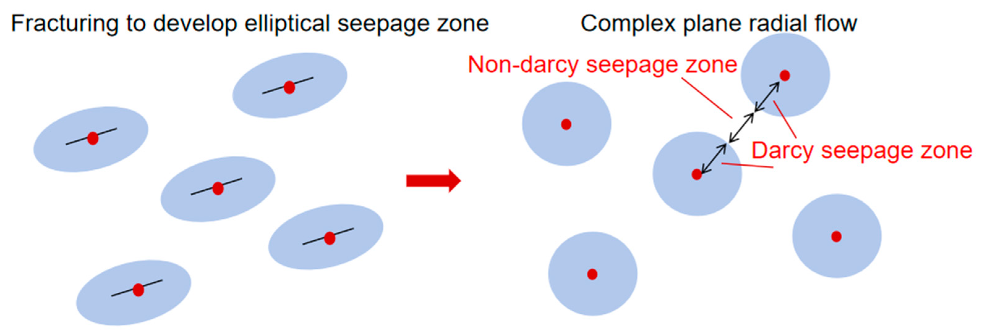
By setting model assumptions, fully applying the radial flow theory, and using the conformal transformation method, the elliptical seepage region is transformed into a circular one. Compared with direct production, fracturing development will form an unutilized region between the oil well reconstruction area, the injection well reconstruction area, and the controlled region of oil and water wells. The transformation of the seepage region in the anti-five-point well pattern fracturing CO₂-flooding is shown in Figure 1. Considering the miscible effect of CO₂ and crude oil, the injection well reconstruction area follows the binomial seepage law, the production well reconstruction area conforms to the Darcy seepage law, and the corresponding formulas are used to calculate the pressure distribution; the original reservoir between the oil and water well reconstruction area follows the nonlinear seepage law. Therefore, the overall model derivation is divided into three regions, each region satisfies the law of conservation of mass and has its own boundary conditions, and each region is coupled by the boundary pressure and mass transfer.

For the production well reconstruction area:

$$\left({\rho }_o{\displaystyle \frac{k_{ro}}{{\mu }_o}}+{\rho }_g{\displaystyle \frac{k_{rg}}{{\mu }_g}}\right)q_{w\_m}-{\rho }_o{\displaystyle \frac{k_{ro}}{{\mu }_o}}{q}_o={\displaystyle \frac{{\varphi }_o{c}_{t\_o}}{k_f{e}^{-e\left(p_o-p_m\right)}}}[{\rho }_0{s}_{o\_o}+{\rho }_g(1-s_{o\_o})]{\displaystyle \frac{\partial p_o}{\partial t}}$$

(1)

where ${\rho }_o$, ${\rho }_g$ are the densities of crude oil and liquid CO₂, respectively, in kg/m³; $k_{ro}$, $k_{rg}$ are the relative permeabilities of the oil phase and liquid CO₂ phase; ${\mu }_o$, ${\mu }_g$ are the viscosities of the oil phase and liquid CO₂ phase, respectively, in mPa·s; $q_{w\_m}$ is the velocity at the junction between the control area of the injection well and the unmodified area, respectively, in m³/d/m; $q_o$ is the intensity of fluid production, respectively, in m³/d/m; ${\varphi }_o$ is the average porosity of the producing well area, respectively, in %; $c_{t\_o}$ is the comprehensive compression coefficient of oil well control area, respectively, in MPa⁻¹; $k_f$ is the permeability of the reconstructed area, respectively, in 10⁻³ μm²; $p_o$ is the static pressure of the reservoir, respectively, in MPa; $p_m$ is the pressure in the untransformed area, respectively, in MPa; $s_{o\_o}$ is the oil saturation in the control zone of the production well.

$$q_0=2k_f{w}_f{h}_e\lambda \left({\displaystyle \frac{k_{ro}}{{\mu }_o}}+{\displaystyle \frac{k_{rg}}{{\mu }_g}}\right)={\displaystyle \frac{(p_{m\_o}-p_{wf}-G_f{r}_{e)}(e^{\mathsf{\Pi }\lambda }-1)}{e^{\mathsf{\Pi }\lambda }+1}}$$

(2)

where $w_f$ is the width of the crack; $h_e$ is the effective thickness of the oil reservoir; $p_{m\_o}$ is the pressure at the junction between the unmodified area and the production well control area, respectively, in MPa; $p_{wf}$ is the bottomhole flow pressure, respectively, in MPa; $r_e$ is the drainage radius.

For the matrix unmodified area:

$$q_{w\_m}-q_{o\_m}={\displaystyle \frac{{\varnothing }_m{c}_{t\_m}}{k_m{e}^{-\alpha (p_{w\_m}-p_{o\_m})}}}{\displaystyle \frac{\partial p_m}{\partial t}}$$

(3)

$$q_m=2\pi k_m({\rho }_o{\displaystyle \frac{k_{ro}}{{\mu }_o}}+{\rho }_g{\displaystyle \frac{k_{rg}}{{\mu }_g}}){\displaystyle \frac{p_{w\_m}-p_{m\_o}-G_{m}d}{d}}$$

(4)

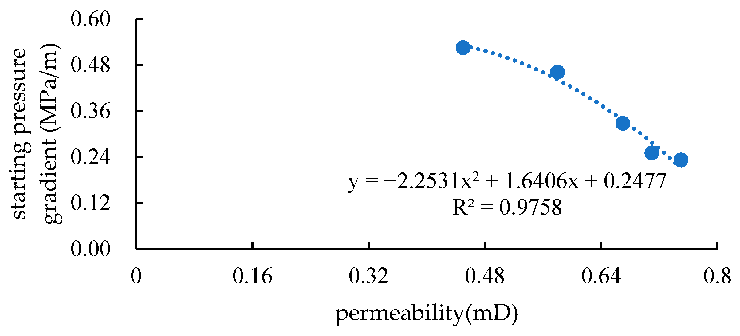
${\varnothing }_m$ is the average porosity of the unmodified area, respectively, in %; $c_{t\_m}$ is the integrated compression coefficient in the control area of the injection well, respectively, in MPa⁻¹; $k_m$ is the permeability of the unmodified area, respectively, in 10⁻³ μm²; α is the sensitive factor in the exponential decay law of the pressure sensitivity effect, in MPa⁻¹; $p_{w\_m}$ is the pressure at the junction between the control area and the unreconstructed area of the injection well, respectively, in MPa; G_m is the starting pressure gradient of the matrix in the unmodified area, in MPa/m; d is the range of the unmodified area, in m.

For the injection well reconstruction area:

$${\rho }_g{\displaystyle \frac{k_{rg}}{{\mu }_g}}{q}_w-\left({\rho }_o{\displaystyle \frac{k_{ro}}{{\mu }_o}}+{\rho }_g{\displaystyle \frac{k_{rg}}{{\mu }_g}}\right)q_{w\_m}={\displaystyle \frac{{\varphi }_w{c}_{t\_w}}{k_f{e}^{-\alpha \left(p_w-p_{wf}\right)}}}[{\rho }_o{s}_{w\_o}+{\rho }_g(1-s_{w\_o})]{\displaystyle \frac{\partial p_w}{\partial t}}$$

(5)

${\varphi }_w$ is the average porosity of the injection well area, respectively, in %; $s_{w\_o}$ is the oil saturation of the injection well control area.

The initial conditions are:

$$p_{w\_m}={p_{m\_o}=p}_i=C_1$$

(6)

$$p_{wf}=C_2$$

(7)

$$q_w=C_3$$

(8)

p_i is the original formation pressure, in MPa; $q_w$ is the injection strength, respectively, in m³/d/m; C₁, C₂, C₃ are the initial condition constants.

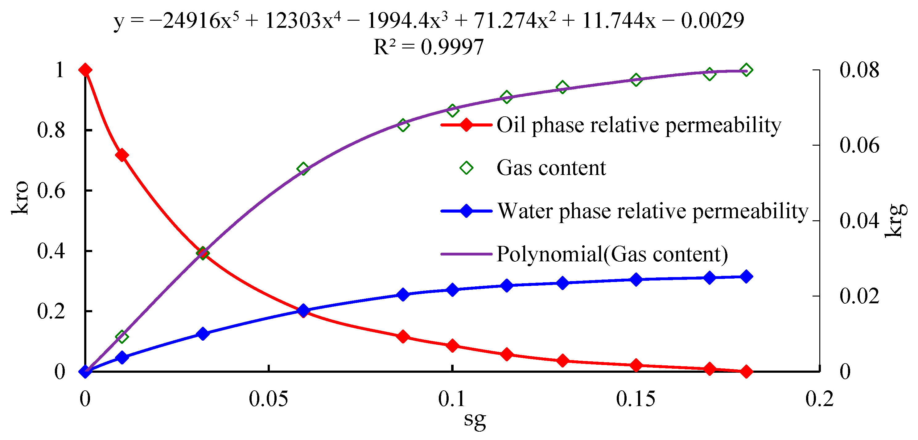
During the CO₂ injection process, there are three-phase seepage of crude oil, supercritical CO₂, and free water underground. Considering that only part of the free water enters the reservoir when the fracturing fluid is injected in the initial stage and is almost completely produced during the flowback period, to ensure the solvability of the model, the multiphase seepage is simplified to two-phase seepage of oil–liquid CO₂.

Based on the physical simulation results of the gas–oil two-phase relative permeability test, and by referring to the derivation process of the oil–water fractional flow equation, a gas–oil ratio calculation model is constructed. The processed phase permeability given by the physical simulation and the relationship graph between the derivative of the gas content and the gas saturation is shown in Figure 2.

By using the gas–oil two-phase gas content fractional flow equation and combining it with the phase permeability, the gas content under any gas saturation can be determined. Therefore, the key to determining the gas–oil ratio is how to determine the gas saturation. The calculation equation for the gas saturation at any time after the gas breakthrough is as follows:

$$f_{{co}_2}^{\prime }{\displaystyle \frac{Q_{{co}_2}}{\pi \varphi h}}=r_2-r_w^2$$

(9)

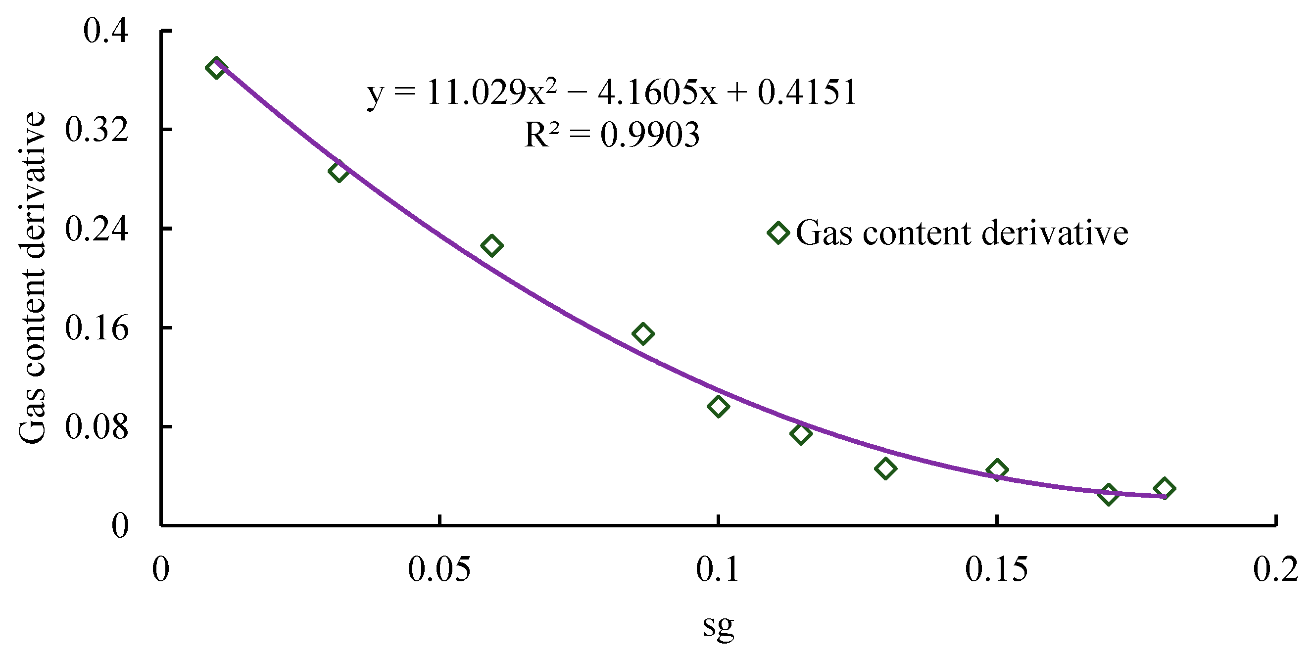
According to the cumulative injection volume at any time, the derivative of the gas content is determined. Then, based on the relationship curve between f_CO2 and $S_g$, the relationship graph between $f_{{co}_2}^{\prime }$ and $S_g$ is established, as shown in Figure 3. By fitting, the functional relationship between $f_{{co}_2}^{\prime }$ and $S_g$ is determined, and the gas saturation at any time is determined according to the root formula:

$$S_g={\displaystyle \frac{4.1605+\sqrt{{4.1605}^2-4\times 11.029\times (0.4151-f_{{co}_2}^{\prime })}}{2\times 11.029}}$$

(10)

By fitting the fractional flow equation, the relationship function between the gas content and the gas saturation is determined. Substituting the gas saturation into the fractional flow equation to determine the gas content, and then converting the gas content into the gas–oil ratio, the gas–oil ratio calculation model after gas breakthrough in CO₂ flooding of tight oil reservoirs is obtained:

$$GOR={\displaystyle \frac{f_{{co}_2}}{1-f_{{co}_2}}}$$

(11)

According to the CO₂ flooding reservoir engineering model, the oil production and gas–oil ratio at any time can be calculated. Combining with their definitions, the development indicators such as the recovery degree and the oil production rate can be determined.

2.2. Semi-Analytic Solution of Mathematical Model

The solution of the above mathematical model mainly includes two parts: one is the change in formation energy caused by the injection and production volumes of the source and sink, and the produced liquid volume continuously changes; the other is to decompose the produced liquid volume into the produced oil volume and the produced gas volume, that is, to determine the gas–oil ratio. The specific semi-analytical solution method is as follows.

Based on the bottom hole flowing pressure of the production well zone and the original formation pressure of the unmodified area, determine the produced liquid volume at the start-up time; according to the mass conservation equation when combined with the unsteady-state pressure distribution formula, determine the pressure change value at the junction of the unmodified area and the oil well zone in the first time step, which is used as the boundary pressure in the next time step. Calculate the injection volume according to the injection intensity of the injection well zone, and combine with the material balance equation. Since the initial pressure at the junction of the injection well zone and the unmodified area is the original formation pressure, the injection volume is all used to increase the pressure in the injection well zone (the specific pressure increase range and the material conservation equation need to be judged whether they are miscible), thereby determining the pressure change value at the bottom hole of the injection well in the first time step. Based on the bottom hole flowing pressure of the injection well in the first time step and the boundary pressure between the injection well zone and the unmodified area, determine the seepage intensity of the injection well zone flowing into the unmodified area (the injection volume does not all flow into the unmodified area, and part is used to restore the formation pressure in the injection well zone). Judge whether there is a flow into the production well zone to supplement energy in the unmodified area according to the pressure difference at both ends of the unmodified area and the starting pressure. If Δp_m > G, there is energy entering the production well zone and the supplement is completed; if Δp_m < G, the injection volume in the injection well zone is insufficient to increase the pressure in the unmodified area to overcome the starting pressure. At this time, the average pressure in the injection well zone continues to rise, and the formation pressure in the production well zone continues to decline until the pressure difference is greater than the starting pressure. Based on the key position index calculation in the first time step, the index in the next time step can be iteratively calculated. Overall, it is manifested as: the pressure in the production well zone decreases; the pressure in the injection well zone rises; the driving system is gradually established in the unmodified area; and the continuous change and solution of the injection volume-produced liquid volume are realized.

Qualitatively judge the miscible driving situation in the injection well zone. The pressure in the injection well zone is high, and the formation pressure conduction is fast after fracturing, so it is easier to form miscible or near-miscible driving. The specific situation is judged by the calculated formation pressure; in the unmodified area, it is partially miscible or immiscible. In the part close to the injection well zone, when the energy propagates, there may be partial miscible driving, while in the part close to the production well zone, the slow pressure propagation leads to immiscible gas–liquid two-phase flow; although the energy in the oil well zone can be supplemented in the later stage, it is difficult to reach the miscible driving of about 28 MPa, and it is in the state of immiscible gas–liquid two-phase flow. Based on this, the multiphase flow state in each region is divided. According to the above method, determine the flow rate in each region at any time, that is, the cumulative injection volume. Judge whether the injected CO₂ phase reaches the production well (that is, whether gas breakthrough occurs) according to the cumulative injection volume. Before gas breakthrough, the production well is in pure oil flow, and the formation pressure declines; after gas breakthrough, calculate the rising derivative of the gas content according to the flow rate, combined with the fitted relationship to determine the gas saturation at the production well position, and then calculate the gas content in reverse, and finally realize the quantitative calculation of the gas–oil ratio. Combine the dynamic calculation results of the gas–oil ratio and the flow rate calculation results to determine the change laws of the oil production and the gas–oil ratio before and after gas breakthrough.

2.3. The Injection Strength Is Established Based on Formation Pressure Stability

Using the above model, the injection intensities to maintain the formation pressure levels in Blocks A and B are determined by trial calculation to be 0.39 t/d/m and 0.63 t/d/m, respectively. The thicknesses of each small layer are statistically analyzed, and the effective thickness data of some layers in the blocks are shown in

Table 1. Statistics of the effective thickness of some layers in typical blocks.

Well Number in Block A	Effective Thickness (m)	Well Number in Block B	Effective Thickness (m)
A-1	12.9	B-1	8.2
A-2	5.8	B-2	17.7
A-3	10.7	B-3	7.3
A-4	3.5	B-4	8.8
A-5	13.3	B-5	13.7

. Combined with the location attributes of the injection wells, the injection rates to maintain the formation pressure are determined to be 24 t/d and 32 t/d, respectively. Through statistical analysis of the injection–production ratio, it can be seen that the reason why the injection–production ratio is greater than 1 when the formation pressure is stable in CO₂ flooding is that there is miscible driving in the injection well zone.

2.4. Injection Intensity Correction Based on Phase Contact Mode

The injection intensity for each block to maintain the formation pressure stability in CO₂ flooding is determined by the reservoir engineering method, but there are problems when directly applied to the scheme design or prediction: first, the reservoir engineering method is a homogeneous model and cannot describe the reservoir heterogeneity; second, the injection intensity correction under the actual reservoir sand body contact relationship is not considered. Therefore, in this subsection, a numerical simulation theoretical model is established to simulate the development effects under different phase contact relationships, and an injection intensity correction factor is proposed to guide the numerical simulation scheme design of the real block.

Combined with the field sedimentary facies data, three sedimentary facies, namely channel, main sheet sand, and non-main sheet sand, are summarized. According to the sand body attributes of different types of sedimentary facies and the drilling conditions of each well, a numerical simulation theoretical model based on different phase contact relationships is established, as shown in Figure 4. The step size is 25 × 25 m, and the schemes and basic parameters are shown in

Table 2. Scheme design table.

Plan	Injection Well	Producing Well
1	Non-main sheet sand	watercourse
2	Non-main sheet sand	Non-main sheet sand
3	watercourse	watercourse
4	watercourse	Non-main sheet sand

and

Table 3. Basic parameter table.

	Injection Well				Producing Well
Scheme	Porosity	Permeability	Effective Thickness	Oil Saturation	Porosity	Permeability	Effective Thickness	Oil Saturation
1	11.1	0.5	0.6	53.7	12.1	0.7	1.6	60.4
2	11.1	0.5	0.6	53.7	11.1	0.5	0.6	53.7
3	12.1	0.7	1.6	60.4	12.1	0.7	1.6	60.4
4	12.1	0.7	1.6	60.4	11.1	0.5	0.6	53.7

. The production curves of each scheme are shown in Figure 5.

2.5. Geological Model

The study area includes the target Block A and the target Block B, which are developed with natural energy. The formation energy declines rapidly, with a decline rate of more than 30%, and the predicted recovery factor is less than 10%. Block A belongs to ultra-low permeability, with underdeveloped fractures and small-scale sand body development, making it difficult to establish an effective driving system. An excessive injection rate will lead to gas channeling, while too slow injection rate will result in slow pressure recovery in the oil well area, inability to supplement the formation energy, and inability to achieve miscibility in the oil well area.

Based on the static data of the target blocks, the parameters required for the model are selected, and the geological models of Block A and Block B are established using the Petrel2021 (Schlumberger, Houston, TX, USA) software. The plane grid step size is 20 m × 20 m, and the three-dimensional grid is generated using the pillar-griding module with the edge of the sedimentary facies as the boundary. The grid processing results of the modeling area are shown in

Table 4. Grid processing results of the modeling area.

Block	A	B
Number of Wells	18	30
Area (km2)	3.04	6.95
Step size (m)	20 × 20	20 × 20
Vertical subdivision (m)	0.2	0.2
Number of grids	181 × 216	277 × 372
Planar node	5.5907 × 107	1.42819 × 108

.

The CMG2021 (for Canada) software is used to perform history matching on the model. The calculation error of the oil production in the whole area is less than 5%, and the error of the formation pressure in the whole area is not more than 4%. The history-matching accuracy meets the prediction requirements.

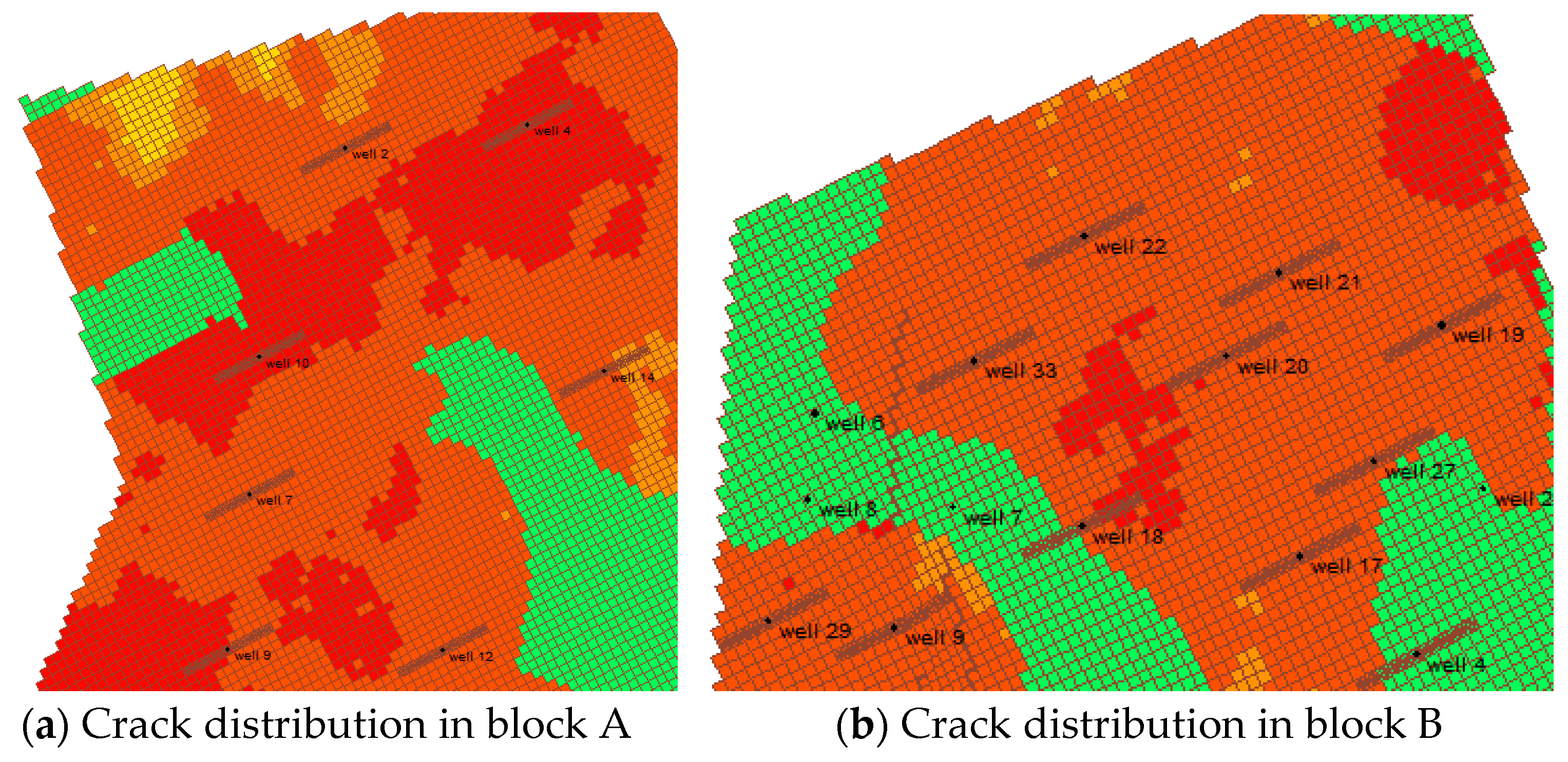
In the fractured development and stimulation zone of tight oil reservoirs, there are main fractures and induced fractures. Based on the fracturing construction summary data provided by the site, the main fractures and the induced fractures in the stimulation zone are simulated using the hydraulic fracturing module in the CMG numerical simulation software. The fracture parameters and setting interfaces of each block are shown in

Table 5. Crack parameters of each block.

Block	A	B
Fracture half-length (m)	150	150
Fracture Angle (°)	NE76.3°	NE76.3°

, and the fracture distribution is shown in Figure 6.

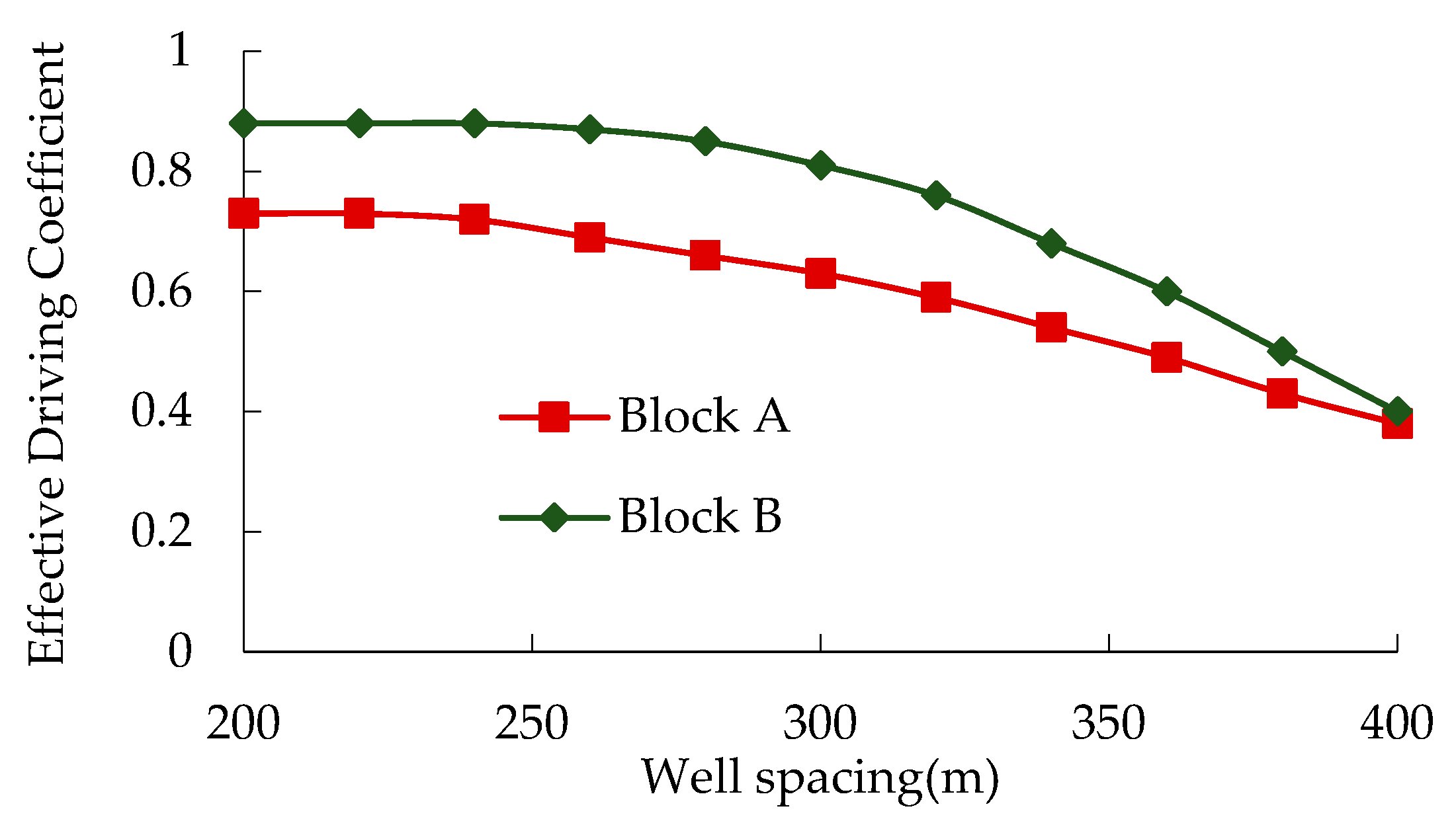
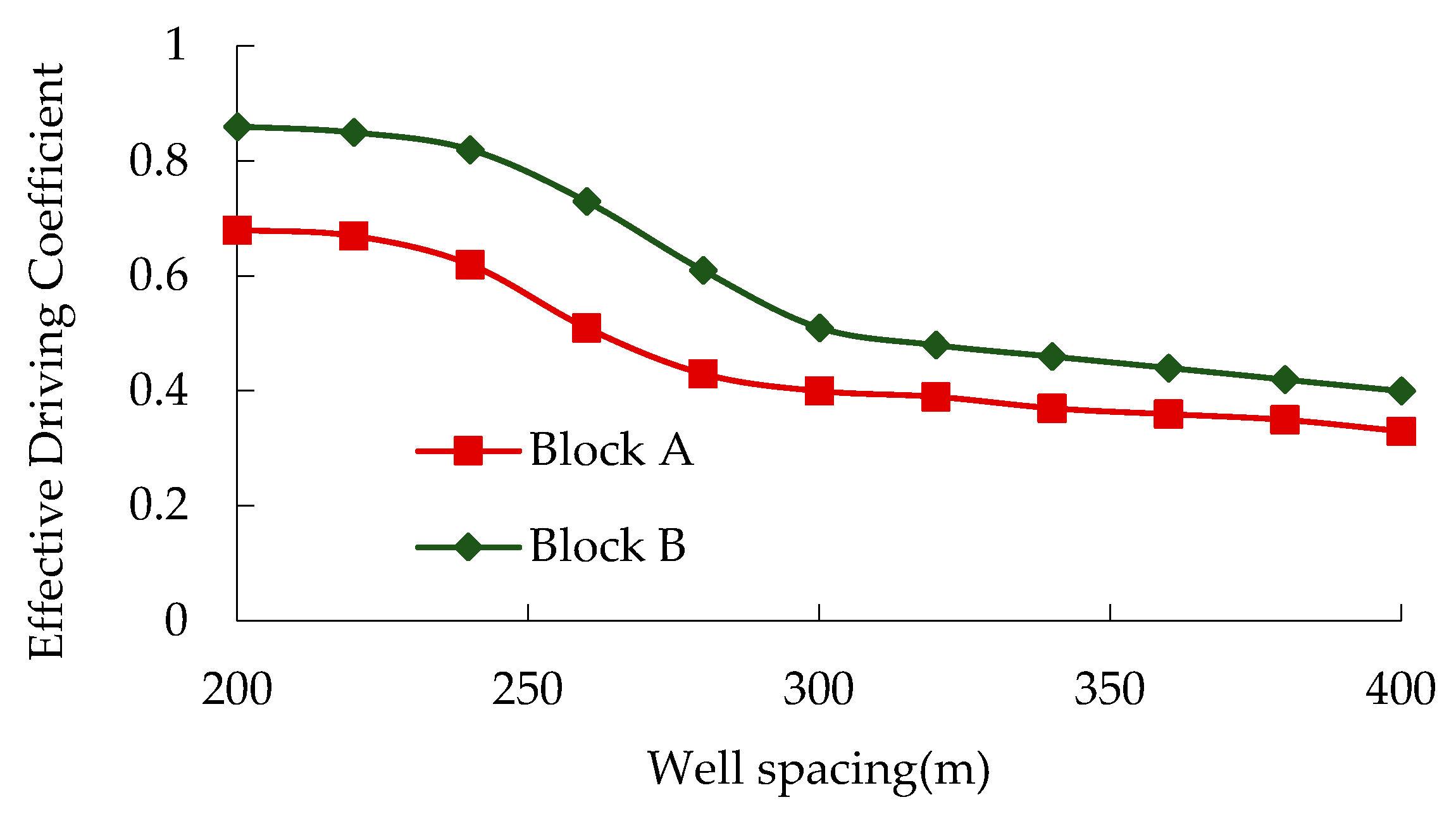
2.6. Determination of Effective Driving Coefficient of Different Well Patterns

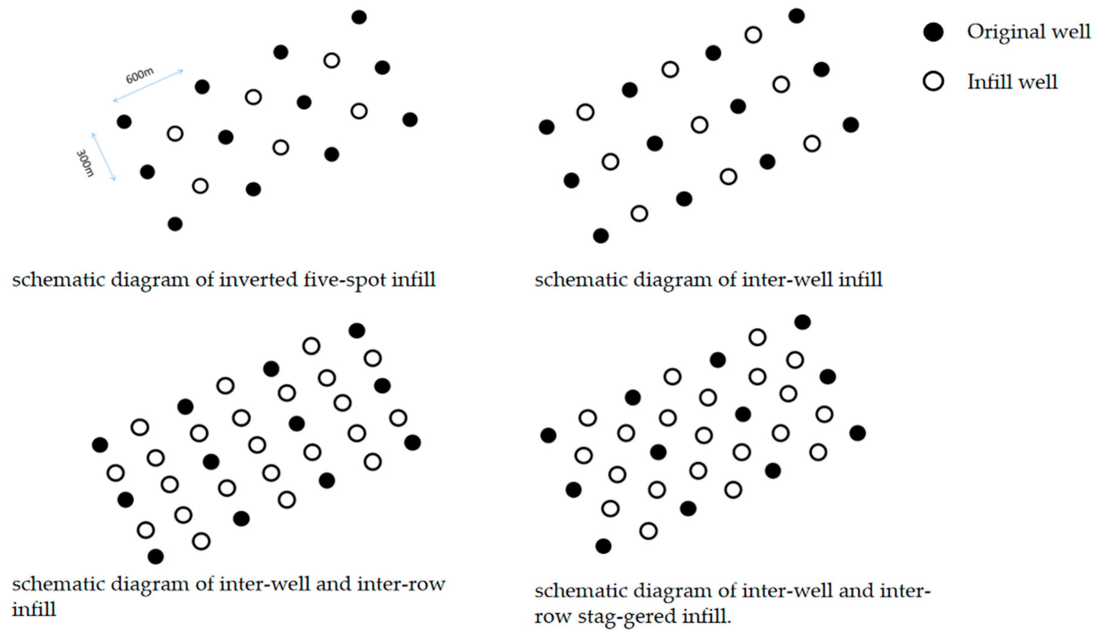
The effective driving coefficient of the well pattern (also known as the utilization coefficient) is the ratio of the producible area to the well pattern area when considering the starting pressure gradient. Based on the possible infill methods and the diamond-shaped anti-nine-point well pattern, the calculation formulas for the effective driving coefficient when the well pattern is consistent with or at an angle to the fracture direction are determined. The results of the anti-five-point method, as a special case of the diamond-shaped anti-nine-point method, are directly given.

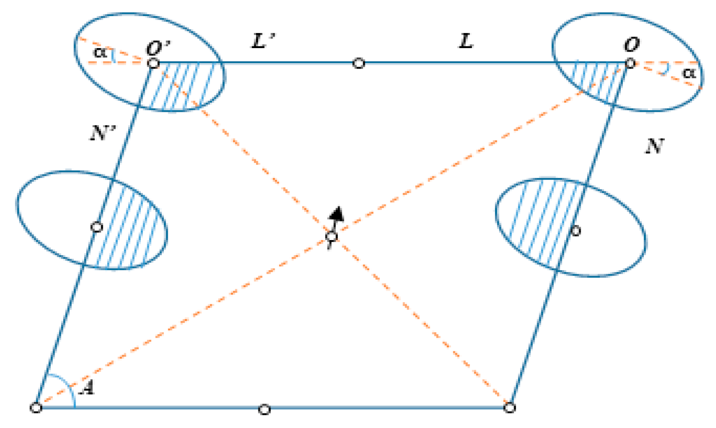
For the well pattern with the well row direction consistent with the fracture direction, the long axis direction of the elliptical seepage field after the oil well fracturing is consistent with the well row direction. Taking the diamond-shaped anti-nine-point well pattern as an example, with the fracture length as the focal length and the radial flow driving radius as the short axis of the ellipse, the sum of the elliptical driving radius and the shaded area formed by the well pattern is the producible area of this well pattern, as shown in Figure 7.

The calculation formula for the effective driving coefficient is:

$$\eta ={\displaystyle \frac{S_g}{S}}$$

(12)

where $S_g$ is the movable area, in m²; S is the control area of the diamond-shaped anti-nine-point well pattern, in m²; $\eta$ is the effective driving coefficient.

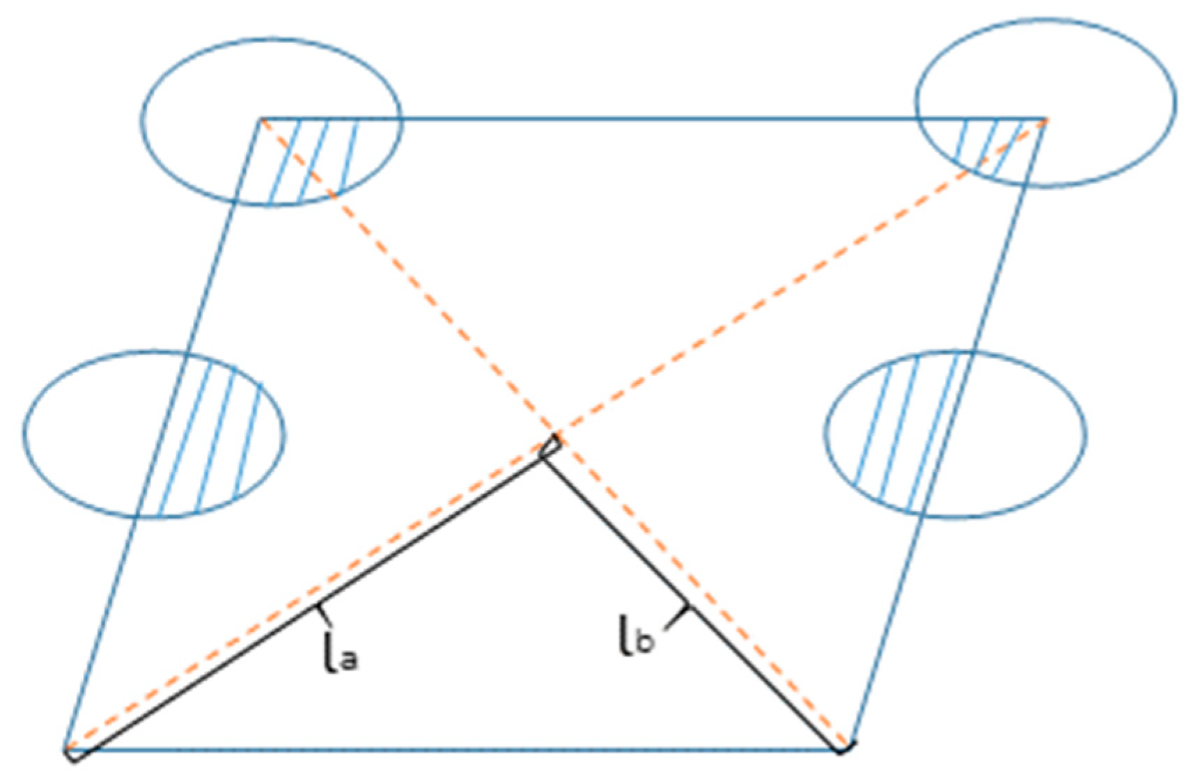
For the well pattern with the well row direction at an angle to the fracture, take the diamond-shaped anti-nine-point well pattern as an example, as shown in Figure 8.

The calculation formula for the effective driving coefficient is:

$$\eta ={\displaystyle \frac{\mathit{S}-2{\mathit{S}}_{\mathit{O}\mathit{N}\mathit{L}}-2{\mathit{S}}_{{\mathit{O}}^{\mathbf{\prime }}{\mathit{N}}^{\mathbf{\prime }}{\mathit{L}}^{\mathbf{\prime }}}-{\mathit{S}}_{\mathit{e}}}{\mathit{S}}}$$

(13)

The five-point well pattern, the diamond-shaped well pattern, and the square anti-nine-point well pattern are all special forms of the above formula. When applied to the calculation of different well patterns, only the angle between the fracture and the well pattern needs to be changed. This formula can be extended to different well patterns in other oilfield blocks.

3. The Boundary of the CO₂ Flooding Pattern in Tight Reservoir Was Established

3.1. Establish the Effective Driving Coefficient

The relationship chart of the startup pressure gradient and permeability is shown in Figure 9. Combining the statistical results of permeability in Block A and Block B, the values of the startup pressure gradient are determined to be 0.53 MPa/m and 0.25 MPa/m, respectively.

The parameters required for the model are determined by integrating the block data, as shown in

Table 6. Calculation parameters of effective driving coefficient for typical blocks.

Basic Parameters	Block A	Block B
Fracture half-length (m)	150	150
Short-axis use distance (m)	50	50
Fracture–well row angle	0.2	0.2
Permeability (10−3 μm2)	0.4	0.7
Startup pressure gradient (MPa/m)	0.53	0.25
Initial formation pressure (MPa)	20.2	20.2
Bottom hole flowing pressure (MPa)	5	5
Porosity (%)	5.3	7.8

. Using the established effective driving coefficient model, the effective driving coefficients of typical blocks under different infill well spacings are calculated, and the effective driving coefficient charts for different infill types in Block A and Block B are presented, respectively, as shown in Figure 10, Figure 11 and Figure 12.

As can be seen from the figures, when the well spacing decreases from 400 m to 200 m, the increasing amplitude of the effective driving coefficient gradually becomes smaller. For the inverted five-spot infill method, inflection points occur at 240 m in Block A and 260 m in Block B, respectively; under the inverted nine-spot infill method, inflection points occur at 280 m in Block A and 300 m in Block B, respectively, and compared with the inverted five-spot method, the increase in well pattern density makes the inflection points appear earlier; under the linear injection–production well row infill method, inflection points occur at 240 m in both Block A and Block B. This method is mainly effective in the short-axis direction. In the initial stage, the reduction of well spacing increases the driving coefficient, and when the inter-row modified areas approach each other, the driving coefficient increases suddenly. The inflection point of the effective driving coefficient curve is determined by the second derivative method combined with engineering criteria. Firstly, the effective driving coefficient–well spacing curve is smoothly interpolated, the second derivative is calculated, and the zero crossing point (extreme point of curvature) of the derivative is taken as the mathematical inflection point. At the same time, the increase in the effective drive factor caused by the reduction of the well spacing is required to be halved to ensure the economic effectiveness of the well pattern density and avoid the cost increase caused by excessive well pattern compaction.

At present, the lower limit of the effective driving coefficient for water flooding in low-permeability reservoirs is 0.7, but the lower limit for CO₂ flooding has not been reported yet. Therefore, taking the inflection points of the relationship charts of the effective driving coefficient and well spacing/row spacing as the boundaries, the lower limits of well spacing and row spacing of the well pattern are determined, as shown in

Table 7. Calculation results of effective driving coefficient for different infill methods.

Infill Method	Block	Well Spacing Limit (m)	Effective Driving Coefficient
Inverted Five-Spot	A	240	0.72
	B	260	0.87
Inverted Nine-Spot	A	280	0.75
	B	300	0.85
Linear Row Spacing	A	240	0.62
	B	240	0.82

.

3.2. Sensitivity Analysis of Key Parameters

A systematic sensitivity analysis was conducted to evaluate how variations in permeability, porosity, and startup pressure gradient affect model predictions. The analysis focused on two critical outcomes: injection intensity and effective driving coefficient.

• Permeability Sensitivity

Permeability demonstrated the highest sensitivity among the parameters. For Block A (permeability = 0.4 × 10⁻³ μm²), a 50% increase in permeability reduced the required injection intensity by 18% (from 0.39 to 0.32 t/d/m) and increased the effective driving coefficient by 12% (from 0.72 to 0.81). Conversely, a 30% permeability reduction in Block B (0.7 → 0.49 ×10⁻³ μm²) increased the injection intensity by 22% (0.63 → 0.77 t/d/m) and decreased the driving coefficient by 9% (0.87 → 0.79). These results are consistent with the theoretical expectation, the higher the permeability, the larger the pore throat radius of the porous medium, and the lower the fluid percolation resistance. Therefore, the injection strength required to maintain the same pressure propagation decreases, and the pressure can be more efficiently transmitted to the distal reservoir, expanding the mobile area, and increasing the effective driving coefficient. A decrease in permeability leads to a narrowing of the pore throat and a surge in flow resistance (the non-Darcy flow effect is more significant). A higher injection intensity is required to overcome the starting pressure gradient, and the pressure propagation speed is slowed down, the mobile area is reduced, and the driving coefficient is decreased. (Figure 9).

2.

Porosity Impact

Porosity variations showed moderate sensitivity. A 10% porosity increase in Block A (5.3% → 5.8%) decreased injection intensity by 7% (0.39 → 0.36 t/d/m) due to higher fluid storage capacity. However, the effective driving coefficient decreased by 4% (0.72 → 0.69) because increased porosity reduced pressure propagation velocity. In Block B (7.8% → 8.6%), similar porosity increases reduced the injection intensity by 5% but improved the driving coefficient by 3% due to better matrix–fluid interaction.

3.

Startup Pressure Gradient Influence

Startup pressure gradient (SPG) had the most significant impact on the driving coefficient. For Block A (SPG = 0.53 MPa/m), a 20% SPG increase reduced the driving coefficient by 15% (0.72 → 0.61) at optimal well spacing. Conversely, Block B (SPG = 0.25 MPa/m) showed only a 6% reduction in coefficient with a similar SPG increase. This highlights the critical role of SPG in overcoming reservoir flow resistance, as modeled in Equations (3) and (4).

4.

Uncertainty Quantification

Monte Carlo simulations were performed with parameter ranges:

• Permeability: ±30% of baseline;
• Porosity: ±15%;
• SPG: ±25%.

The results indicate 95% confidence intervals for injection intensity:

• Block A: 0.32–0.46 t/d/m;
• Block B: 0.51–0.75 t/d/m.

The effective driving coefficient ranges:

• Block A: 0.65–0.80;
• Block B: 0.80–0.92.

These intervals suggest that permeability and SPG are the primary sources of uncertainty, as their variations directly affect flow resistance and pressure propagation dynamics (Figure 10, Figure 11 and Figure 12).

4. Application of Typical Block Models

4.1. Depletion Mining

Based on the parameter limits of different types of well patterns, and combining the original well pattern well location distribution in typical blocks and the actual requirements of the oilfield, the infill plans for Block A and Block B are carefully designed, covering four infill methods: inverted five-spot infill, inter-well infill, inter-well and inter-row infill, and inter-well and inter-row staggered infill, as shown in Figure 13. Subsequently, the development indicators of continuous depletion development for 15 years after well pattern infill are predicted using the numerical simulation method.

In accordance with the lower limits of well spacing and row spacing derived from the effective driving coefficient model for Block A, and adhering to the principles of well pattern design, this study employed numerical simulation to predict development indicators. Specifically, Figure 14 illustrates the temporal variation of the average daily oil production per well under different infill strategies. The horizontal axis represents time (unit: years), denoting the predicted time span, while the vertical axis shows the average daily oil production per well (unit: t/d), intuitively depicting the daily oil production of each infill strategy at various time points. Figure 15 presents a comparison of the cumulative oil production and incremental oil production over a 15-year development cycle for different infill strategies. The horizontal axis lists various infill methods, including inverted five-spot infill, inter-well infill, inter-well and inter-row infill, and inter-well and inter-row staggered infill. The vertical axis represents the cumulative oil production/incremental oil production (unit: t), clearly demonstrating the total oil production and production enhancement amplitude of each infill strategy over the 15-year period. The results clearly show that, from the perspective of average incremental oil production per well, compared with continuous depletion mining, the inter-well and inter-row infill has the most significant oil-increasing effect, while the inverted five-spot infill has the least.

For Block B, the production rate vs. time chart and the cumulative oil production/incremental oil production histogram are also drawn (as shown in Figure 16 and Figure 17). Through analysis, it can be seen that, from the perspective of average incremental oil production per well, compared with continuous depletion, the inter-well and inter-row staggered infill has the most oil-increasing effect, and the inter-well and inter-row infill has the least.

4.2. Infill Mining

To determine the optimal infill method, the development effect of CO₂ energy supplementation 2 years after infill in typical blocks is predicted.

Comparing the development effects of Block A with different infill methods under depletion development for 15 years, the production rate and incremental oil production change curves are carefully drawn, as shown in Figure 18 and Figure 19. The remaining oil reserve abundance and formation pressure distribution maps are shown in Figure 20 and Figure 21. In terms of average daily oil production per well, the inverted five-spot infill is the highest, followed by the inter-well and inter-row infill, and the inter-well and inter-row staggered infill and inter-well infill are relatively low, with initial values of 1.63 t/d, 1.58 t/d, 1.53 t/d, and 1.51 t/d, respectively. The inverted five-spot infill wells control a large amount of reserves and have the highest production during the depletion period; the inter-well and inter-row infill wells are developed by fracturing, and the drainage range intersects with the original well pattern, with a relatively large fracturing scale, so the production is at the middle level; the inter-well infill has the lowest production due to the limited fracturing scale. After conversion to injection, the production order remains the same, with the inverted five-spot being the highest, followed by the inter-well and inter-row infill, the inter-well and inter-row staggered infill, and the inter-well infill being relatively low, with values of 1.91 t/d, 1.84 t/d, 1.76 t/d, and 1.706 t/d, respectively. The fracture direction of the inverted five-spot is consistent with the injection–production direction, so the conversion to injection is effective quickly and the peak value is high; the inter-well and inter-row infill have a small row spacing, and the wells are first energized to increase oil production, but the wells with a large row spacing have poor effectiveness and less oil-increasing, so the comprehensive peak value is at the middle level; the inter-well infill is effective in the short-axis direction after conversion to injection and needs to overcome the matrix pressure drop outside the drainage radius, so the peak value is the lowest. After infill, the inverted five-spot infill has the highest average incremental oil production per well, so the inverted five-spot infill plan is preferred.

Comparing the development effects of Block B with different infill methods under depletion development for 15 years, the production rate and incremental oil production change curves are shown in Figure 22 and Figure 23, and the remaining oil reserve abundance is shown in Figure 24 and Figure 25. The average daily oil production per well of the inverted five-spot is the highest, followed by the inter-well infill, and the inter-well and inter-row infill and the inter-well and inter-row staggered infill are relatively low, with initial values of 2.37 t/d, 2.34 t/d, 2.35 t/d, and 2.27 t/d, respectively. After conversion to injection, the production rate of the inverted five-spot is the highest, followed by the inter-well and inter-row infill, the inter-well and inter-row staggered infill, and the inter-well infill is relatively low, with values of 3.41 t/d, 3.25 t/d, 3.17 t/d, and 3.13 t/d, respectively. The inverted five-spot has the most incremental oil production; therefore, the inverted five-spot method is determined as the optimal infill method for Block B.

The inverted five-point well pattern maximizes the CO₂ displacement efficiency and reserve control through well placement design aligned with fracture direction, well spacing optimization based on effective drive factor, and efficient pressure conduction due to high permeability. Other well patterns resulted in reduced seepage efficiency and residual oil retention due to deviation in well drainage direction, unreasonable well spacing, or heterogeneity, which verified the necessity of the geo-engineering collaborative optimization method proposed in this study.

5. Discussions

The simplified assumptions of current models (e.g., ignoring the retention water phase of fracturing residues) are suitable for clean reservoirs with thorough fracturing flowback. However, in complex scenarios with high water saturation, more attention should be paid to the fine characterization of multiphase flow mechanisms. In the future, the oil–gas–water three-phase percolation model can be introduced and CT scanning technology can be combined to dynamically quantify the evolution of water phase distribution, so as to solve the shortcomings of the existing model in describing the influence of fracturing fluid residue and formation primary water (Figure 2 phase percolation curve only considers oil–CO₂ two-phase). In view of the surface adsorption effect prevailing in the micro-nano pore throat of low permeability reservoir, it is suggested to introduce the Langmuir adsorption term into the flow equation to correct the influence of CO₂ adsorption retention on the clay mineral surface on the effective permeability, and further improve the applicability of the model under ultra-low permeability conditions (Equations (1)–(5) does not include the mass conservation correction term caused by adsorption).

In terms of reservoir heterogeneity characterization, the current model adopts the assumption of the homogeneous matrix and does not describe the differences in micro/nano pore structure and fracture–matrix coupling flow. Subsequently, the pore structure parameters obtained by CT scanning can be combined to construct a dual-medium model or a random heterogeneous field to quantify the coupling relationship between capillary force, slippage effect and see-through resistance at the pore throat scale (Figure 9 Starting pressure gradient does not distinguish the differences at different pore throat scales). It is worth noting that mineral dissolution induced by CO₂ injection (e.g., feldspar-carbonate dissolution) may lead to pore throat expansion or blockage, leading to the dynamic decline of permeability. However, existing models do not consider such chemical–mechanical coupling effects (permeability is fixed in Equations (3) and (4)). In the future, a reaction–percolation–stress coupling model can be introduced to quantify the effect of mineral alteration on percolation parameters combined with X-ray diffraction experimental data.

In terms of technical optimization, the current research does not involve the alternating water and gas (WAG) injection strategy, but field practice shows that this process can improve oil displacement efficiency by reducing CO₂ fluidity and delaying gas channelization. It is suggested that the integrated component model be further studied to quantify the synergistic effects of CO₂ dissolution and water retention on reservoir wettability and permeability curve under WAG injection, and to improve the multi-objective optimization system of “CO₂ storage capacity, recovery efficiency and gas channelization risk”. The above expansion directions are based on the current three-zone model, and their simplification strategies (such as dividing the see-through zone into the transformed zone and unused zone) balance the mathematical solvability and engineering practicability and provide a scalable theoretical starting point for model iteration in complex scenarios, which conforms to the tight reservoir modeling paradigm of “idealized model → semi-analytical solution → fully coupled numerical simulation”.

6. Conclusions

This study presents a geological–engineering synergistic framework for optimizing CO₂ flooding well patterns in tight oil reservoirs, integrating theoretical modeling, numerical simulation, and field validation. The key findings are summarized as follows:

A semi-analytical model incorporating startup pressure gradients and miscible/immiscible two-phase flow was developed to dynamically calibrate injection strategies. By dividing the reservoir into three regions—modified injector/producer zones and an unmodified matrix zone—the model quantifies pressure distribution and flow resistance under non-Darcy seepage. Field validation in Blocks A and B determined the optimal injection intensities of 0.39 t/d/m and 0.63 t/d/m, respectively, which maintain formation pressure stability while minimizing gas channeling risks. Adjusting the injection rates for the sedimentary facies enhances miscible efficiency by 15–20%, bridging reservoir heterogeneity and engineering feasibility.

A novel effective driving coefficient (η) model was proposed, integrating reservoir heterogeneity (permeability, porosity) and fracture orientation (NE76.3°). By defining η as the ratio of the producible area to the well pattern control area and using second-derivative analysis to identify inflection points, the study determined the lower limits for inverted five-spot well spacing: 240 m (Block A, η = 0.72) and 260 m (Block B, η = 0.87).

The proposed methodology establishes a reproducible technical pathway for integrating CO₂ storage with enhanced oil recovery (EOR), achieving bidirectional optimization of environmental and economic benefits.

In summary, this research provides a foundational framework for maximizing CO₂ utilization efficiency in tight oil reservoirs, with direct implications for improving recovery factors and advancing carbon neutrality objectives through strategic well pattern design.

References

1. Liu, Y.; Tang, H.; Muhammad, A.; Huang, G. Emission Mechanism and Reduction Countermeasures of Agricultural Greenhouse Gases—A Review. Greenh. Gases Sci. Technol. 2019, 9, 160–174. [Google Scholar] [CrossRef]
2. Kongboon, R.; Gheewala, S.H.; Sampattagul, S. Greenhouse Gas Emissions Inventory Data Acquisition and Analytics for Low Carbon Cities. J. Clean. Prod. 2022, 343, 130711. [Google Scholar] [CrossRef]
3. Sharma, S.; Bhattacharya, S.; Garg, A. Greenhouse Gas Emissions from India: A Perspective. Curr. Sci. 2006, 90, 326–333. [Google Scholar]
4. Guo, J.; Zhou, C. Greenhouse Gas Emissions and Mitigation Measures in Chinese Agroecosystems. Agric. For. Meteorol. 2007, 142, 270–277. [Google Scholar] [CrossRef]
5. Apergis, N.; Majeed, M.T. Greenhouse Gas Emissions and Cross-National Happiness: A Global Perspective. Air Qual. Atmos. Health 2021, 14, 1289–1300. [Google Scholar] [CrossRef]
6. Courtney, T.; Westfield, I.; Ries, J.B. CO2-Induced Ocean Acidification Impairs Calcification in the Tropical Urchin Echinometra Viridis. J. Exp. Mar. Biol. Ecol. 2013, 440, 169–175. [Google Scholar] [CrossRef]
7. Chakraborty, K.; Joshi, A.P.; Ghoshal, P.K.; Baduru, B.; Sarma, S.; Metzl, N.; Gehlen, M.; Chevallier, F.; Monaco, C.L. Indian Ocean Acidification and Its Driving Mechanisms over the Last Four Decades (1980–2019). Glob. Biogeochem. Cycles 2024, 38, e2024GB008139. [Google Scholar] [CrossRef]
8. Yildiz, G. Physiological Impacts of CO2-Induced Acidification and UVR on Invasive Alga Caulerpa Racemosa. Ocean Sci. J. 2024, 59, 11. [Google Scholar] [CrossRef]
9. Lapola, D.M.; Blanco, C.C.; Cardeli, B.R.; Esquivel-Muelbert, A.; Martinelli, J.V.; Quesada, C.N.A.; Rius, B.F.; Silva-Junior, C.H.L. Not Just Semantics: CO2 Fertilization Can Be a Disturbance Leading to Worldwide Forest Degradation. Plants People Planet 2025, 7, 638–648. [Google Scholar] [CrossRef]
10. Chen, X.; Zhang, Q.; Trivedi, J.; Li, Y.; Liu, J.; Liu, Z.; Liu, S. Investigation on Enhanced Oil Recovery and CO2 Storage Efficiency of Temperature-Resistant CO2 Foam Flooding. Fuel 2024, 364, 130870. [Google Scholar] [CrossRef]
11. Kovscek, A.R.; Cakici, M.D. Geologic Storage of Carbon Dioxide and Enhanced Oil Recovery. II. Cooptimization of Storage and Recovery. Energy Convers. Manag. 2005, 46, 1941–1956. [Google Scholar] [CrossRef]
12. Qi, S.; Yu, H.; Xie, F.; Hu, M.; Lu, J.; Wang, Y. Experimental Investigation on the CO2 Effective Distance and CO2-EOR Storage for Tight Oil Reservoir. Energy Fuels 2022, 37, 339–349. [Google Scholar] [CrossRef]
13. Farajzadeh, R.; Eftekhari, A.A.; Dafnomilis, G.; Lake, L.W.; Bruining, J. On the Sustainability of CO2 Storage through CO2—Enhanced Oil Recovery. Appl. Energy 2020, 261, 114467. [Google Scholar] [CrossRef]
14. Chen, H. Key Problems and Countermeasures in CO2 Flooding and Storage. Acta Geol. Sin. Engl. Ed. 2023, 97, 858–872. [Google Scholar] [CrossRef]
15. Al-Mamoori, A.; Krishnamurthy, A.; Rownaghi, A.A.; Rezaei, F. Carbon Capture and Utilization Update. Energy Technol. 2017, 5, 834–849. [Google Scholar] [CrossRef]
16. Bashir, A.; Ali, M.; Patil, S.; Aljawad, M.S.; Mahmoud, M.; Al-Shehri, D.; Hoteit, H.; Kamal, H.S. Comprehensive Review of CO2 Geological Storage: Exploring Principles, Mechanisms, and Prospects. Earth-Sci. Rev. 2024, 249, 104672. [Google Scholar] [CrossRef]
17. Agartan, E.; Gaddipati, M.; Yip, Y.; Savage, B.; Ozgen, C. CO2 Storage in Depleted Oil and Gas Fields in the Gulf of Mexico. Int. J. Greenh. Gas Control 2018, 72, 38–48. [Google Scholar] [CrossRef]
18. Ding, M.; Wang, Y.; Liu, D.; Wang, X.; Zhao, H.; Chen, W. Enhancing Tight Oil Recovery Using CO2 Huff and Puff Injection: An Experimental Study of the Influencing Factors. J. Nat. Gas Sci. Eng. 2021, 90, 103931. [Google Scholar] [CrossRef]
19. Shen, A.; Liu, Y.; Wang, X.; Cai, B.; He, C.; Liang, S. The Geological Characteristics and Exploration of Continental Tight Oil: An Investigation in China. J. Pet. Explor. Prod. Technol. 2019, 9, 1651–1658. [Google Scholar] [CrossRef]
20. Du, J.; Liu, H.; Ma, D.; Fu, J.; Wang, Y.; Zhou, T. Discussion on Effective Development Techniques for Continental Tight Oil in China. Pet. Explor. Dev. 2014, 41, 217–224. [Google Scholar] [CrossRef]
21. Zhu, R.; Zou, C.; Mao, Z.; Yang, H.; Xiao, H.; Wu, S.; Cui, J.; Su, L.; Li, S.; Yang, Z. Characteristics and Distribution of Continental Tight Oil in China. J. Asian Earth Sci. 2019, 178, 37–51. [Google Scholar] [CrossRef]
22. Wang, R.; Lun, Z.; Lyu, C.; Wang, Y.; Tang, Y.; Wang, X. Research status and development trends of worldwide new technologies for enhanced oil recovery. Pet. Geol. Recovery Effic. 2021, 28, 81–86. [Google Scholar] [CrossRef]
23. Li, Y.; Huang, W.; Jin, Y.; He, Y.; Chen, Z.; Tang, Y.; Wu, G. Different reservoir types of CO2 flooding in Sinopec EOR technology development and application under “dual carbon” vision. Pet. Reserv. Eval. Dev. 2021, 11, 793–804. [Google Scholar] [CrossRef]
24. Li, Y. Technical advancement and prospect for CO2 flooding enhanced oil recovery in low permeability reservoirs. Pet. Geol. Recovery Effic. 2020, 27, 1–10. [Google Scholar] [CrossRef]
25. Kong, B.; Wang, S.; Chen, S. Simulation and Optimization of CO2 Huff-and-Puff Processes in Tight Oil Reservoirs. In Proceedings of the SPE Improved Oil Recovery Conference, Tulsa, OK, USA, 11–13 April 2016. [Google Scholar] [CrossRef]
26. Ji, B.; He, Y. Practice and understanding about CO2 flooding in low permeability oil reservoirs by Sinopec. Pet. Reserv. Eval. Dev. 2021, 11, 805–811. [Google Scholar] [CrossRef]
27. Kukharova, T.; Maltsev, P.; Novozhilov, I. Development of a Control System for Pressure Distribution During Gas Production in a Structurally Complex Field. Appl. Syst. Innov. 2025, 8, 51. [Google Scholar] [CrossRef]
28. Wang, T.; Wang, L.; Meng, X.; Chen, Y.; Song, W.; Yuan, C. Key Parameters and Dominant EOR Mechanism of CO2 Miscible Flooding Applied in Low-Permeability Oil Reservoirs. Geoenergy Sci. Eng. 2023, 225, 211724. [Google Scholar] [CrossRef]
29. Yao, T.; Sun, L.; Cui, C. Optimization Design of CO2 Huff-n-Puff Parameters in Fuyu Tight Reservoir. Spec. Oil Gas Reservoirs. 2024, 31, 123–128. [Google Scholar]
30. Zhu, W.; Liu, J.; Song, H.; Sun, Y.; Wang, M. Calculation of effective startup degree of non-Darcy flow in low or ultra-low permeability reservoirs. Acta Pet. Sin. 2010, 31, 452–457. [Google Scholar] [CrossRef]
31. Chi, J.; Ju, B.; Lyu, G.; Zhang, X.; Wang, J. A Computational Method of Critical Well Spacing of CO2 Miscible and Immiscible Concurrent Flooding. Pet. Explor. Dev. 2017, 44, 815–823. [Google Scholar] [CrossRef]
32. Chi, J.; Ju, B.; Wang, J.; Zhang, X.; Chen, W.; Zhang, M. A Novel Numerical Simulation of CO2 Immiscible Flooding Coupled with Viscosity and Starting Pressure Gradient Modeling in Ultra-Low Permeability Reservoir. Front. Earth Sci. 2023, 17, 884–898. [Google Scholar] [CrossRef]
33. Zhang, N.; Yin, M.; Wei, M.; Bai, B. Identification of CO2 Sequestration Opportunities: CO2 Miscible Flooding Guidelines. Fuel 2019, 241, 459–467. [Google Scholar] [CrossRef]
34. Sun, H.; Xiong, F.; Wu, Z.; Ji, J.; Fan, L. An Extended Numerical Manifold Method for Two-Phase Seepage–Stress Coupling Process Modelling in Fractured Porous Medium. Comput. Methods Appl. Mech. Eng. 2022, 391, 114514. [Google Scholar] [CrossRef]
35. Li, S.; Sun, L.; Chen, Z.; Li, J.; Tang, Y.; Pan, Y. Further discussion on reservoir engineering concept and development mode of CO2 flooding-EOR technology. Pet. Reserv. Eval. Dev. 2020, 10, 1–14. [Google Scholar] [CrossRef]
36. Li, Z.; Lyu, W.; Wang, H.; Li, M.; Chen, T.; Zheng, Z. Influence of injector-producer deployment pattern on development effect of CO2 flooding in low-permeability reservoirs with areal heterogeneity. Pet. Geol. Oilfield Dev. Daqing 2024, 43, 149–157. [Google Scholar]
37. Luo, E.; Hu, Y.; Li, B.; Wang, J.; Wang, Z. Methods of improving sweep volume by mobility control for CO2 flood in foreign countries. Oilfield Chem. 2013, 30, 613–619. [Google Scholar]
38. Collier, T.S. State of the Art Installation of CO2 Injection Equipment: A Case Study. In Proceedings of the Permian Basin Oil and Gas Recovery Conference, Midland, TX, USA, 10–11 March 1988. [Google Scholar] [CrossRef]
Figure 1. Transformation of the seepage region in the anti-five-point well pattern fracturing CO2 flooding.
Sustainability 17 04751 g001
Figure 2. Relationship curves of gas–oil phase permeability and the derivative of gas content with gas saturation.
Sustainability 17 04751 g002
Figure 3. Relationship curve between the derivative of gas content and gas saturation.
Sustainability 17 04751 g003
Figure 4. Theoretical model.
Sustainability 17 04751 g004
Figure 5. Oil production curve: (a) watercourse × watercourse contact oil production; (b) watercourse × non-main sheet sand contact oil production; (c) non-main sheet sand × non-main sheet sand contact oil production; (d) non-main sheet sand × watercourse contact oil production.
Sustainability 17 04751 g005
Figure 6. Crack distribution.
Sustainability 17 04751 g006
Figure 7. Schematic diagram of the seepage region around the oil well (the well row direction is consistent with the fracture direction).
Sustainability 17 04751 g007
Figure 8. Schematic diagram of the seepage region around the oil well (the well row direction is inconsistent with the fracture direction).
Sustainability 17 04751 g008
Figure 9. Relationship chart of startup pressure gradient and permeability.
Sustainability 17 04751 g009
Figure 10. Inverted five-spot infill.
Sustainability 17 04751 g010
Figure 11. Inverted nine-spot infill.
Sustainability 17 04751 g011
Figure 12. Linear gas injection well row infill.
Sustainability 17 04751 g012
Figure 13. Schematic diagrams of infill.
Sustainability 17 04751 g013
Figure 14. Production rate chart of different infill methods for Block A.
Sustainability 17 04751 g014
Figure 15. Cumulative/incremental oil production histogram of different infill methods for Block A.
Sustainability 17 04751 g015
Figure 16. Production rate chart of different infill methods for Block B.
Sustainability 17 04751 g016
Figure 17. Cumulative/incremental oil production histogram of different infill methods for Block B.
Sustainability 17 04751 g017
Figure 18. Production rate.
Sustainability 17 04751 g018
Figure 19. Incremental oil production.
Sustainability 17 04751 g019
Figure 20. Current remaining oil reserve abundance map of inverted five-spot infill for Block A.
Sustainability 17 04751 g020
Figure 21. Remaining oil reserve abundance map of inverted five-spot infill after 15 years for Block A.
Sustainability 17 04751 g021
Figure 22. Production rate of different infill methods.
Sustainability 17 04751 g022
Figure 23. Incremental oil production histogram of different infill methods.
Sustainability 17 04751 g023
Figure 24. Current remaining oil reserve abundance map of inverted five-spot infill for Block B.
Sustainability 17 04751 g024
Figure 25. Remaining oil reserve abundance map of inverted five-spot infill after 15 years for Block B.
Sustainability 17 04751 g025