Pathways to Improve Energy Conservation and Emission Reduction Efficiency During the Low-Carbon Transformation of the Logistics Industry

Abstract

Improving logistics efficiency is a central goal in the green transformation of logistics. However, traditional efficiency measurement approaches fail to distinguish the respective impacts of energy conservation efficiency and emission reduction efficiency on overall green logistics efficiency. Thus, based on the NDDF-DEA, this study develops a new logistics efficiency evaluation model, which incorporates the energy structure. The model separately measures overall logistics efficiency, energy conservation efficiency, and emission reduction efficiency. Empirical results show that overall logistics efficiency reaches its highest level when energy conservation efficiency and emission reduction efficiency are aligned. In contrast, a gap between energy conservation efficiency and emission reduction efficiency often leads to lower overall efficiency. The proposed model introduces a new approach to evaluating green logistics efficiency and highlights that emission reduction could be a critical, limiting factor in the green transformation of logistics. In order to identify high-efficiency development pathways for the logistics industry, this study employs fs-QCA to explore four distinct configurations under multiple influencing factors. The results provide valuable insights and policy implications for governments and enterprises aiming to advance the sustainable transformation of logistics.

1. Introduction

Energy is commonly regarded as a fundamental driver of economic development. However, the logistics industry remains heavily reliant on non-renewable energy sources. According to the China Green Logistics Development Report, transportation accounts for approximately 85% of the total energy consumption in the logistics industry [1]. In 2021, the logistics industry consumed around 440 million tons of standard coal, with natural gas comprising only 2.33% of the total [2]. Zeng et al. [3] proposed that the high proportion of coal and oil in the energy structure not only exacerbates the contradiction between energy supply and demand, but also undermines the equilibrium between economic growth and environmental protection.

The high energy consumption and pollution are two fundamental issues hindering the green transformation of the logistics industry. To reduce energy use, companies adopt technological innovations to enhance energy efficiency. However, the increased demand driven by efficiency improvements may ultimately lead to higher overall resource consumption [4]. Many enterprises prioritize energy savings due to their direct impact on economic costs, often placing less emphasis on emissions reduction [5]. This distinction underscores the fact that energy conservation efficiency (ECE) and emission reduction efficiency (ERE) are not entirely equivalent [6]. Jimenez et al. [7] found that while improving energy efficiency in shipping is an important means of achieving emission reduction targets, the two are not entirely equivalent. Moreover, this inconsistency is amplified as the proportion of coal and oil in the energy structure increases, which is already evident in industrial processes [8]. Although improvements in energy efficiency can be achieved, they do not address the core issue and may even widen the gap between energy conservation and emission reduction. Previous studies on logistics efficiency have typically treated energy conservation and emission reduction as a whole. Therefore, this study proposes a logistics efficiency model that separately evaluates energy conservation and emission reduction. It further explores the relationship between overall logistics efficiency and the consistency between energy saving and emission reduction.

In previous studies on logistics efficiency evaluation, Markovits and Bokor [9] indicated that various methods exist for evaluating efficiency and performance, with data envelopment analysis (DEA) offering particular applicability and advantages in the field of logistics. Zheng et al. [10] used DEA to evaluate the logistics efficiency of various provinces along China’s Belt and Road. Yang et al. proposed that economic development disparities always lead to logistics efficiency differences [11]. These studies used the DEA model to measure logistics efficiency while incorporating the economic indicator.

Subsequently, some scholars have advocated for integrating environmental indicators into the evaluation of low-carbon logistics efficiency [12,13]. However, traditional DEA models do not account for undesirable outputs, such as carbon dioxide, which are a by-product of the logistics process [14]. To address this limitation, Zhou et al. relaxed the requirement for proportional changes between desirable and undesirable outputs, developed the non-radial Directional Distance Function (NDDF) model [15]. The non-radial DEA introduces slack variables to assess efficiency more comprehensively, thereby effectively addressing this challenge [16]. Based on the NDDF model, Yao et al. [17] evaluated the logistics efficiency of the industry across 30 Chinese provinces and found that green efficiency levels are closely associated with geographical location. By considering both energy input indicators and emissions output indicators, Qin and Qi [18], as well as Liang et al. [19], separately used a three-stage DEA to evaluate the logistics efficiency in Northwest China and Jiangsu Province.

Table 1. Common DEA models for efficiency evaluation.

	Type of Energy Input	DEA Model Type	Carbon Emissions	Analysis Method of Influencing Factors	Efficiency Level	Regional Differences	Efficiency Trends
Storto and Evangelista [14]	One type	Radial	As output
Park et al. [13]	One type		As output
Zhou et al. [15], Dakpo et al. [16]	One type	Non-radial	As output
Yao et al. [17]	One type	Non-radial	As output	Machine learning models	Overall low	High in the East and low in the West
Qin and Qi [18], Liang et al. [19]	One type	Radial	As input	Stochastic frontier analysis
Lu et al. [20]	One type	Radial	As output	Fs-QCA	Overall low	High in the East and low in the West	Slowly rising
Chen et al. [21]	One type	Radial	As output	Pearson correlation analysis	Overall low	High in the East and low in the West	Fluctuation rise
Xin et al. [22]	One type	Radial	As output	Efficiency decomposition	Comprehensive efficiency not high	High in the East and low in the West	Slowly rising
Zhang et al. [23]	Many type		As output	Tobit model

provides a comparison of various DEA models used in efficiency evaluation. Research on China’s logistics efficiency often employs radial DEA models at the provincial level. Overall, logistics efficiency remains low but shows a slow upward trend over time, with a clear regional pattern of higher efficiency in the eastern regions and lower efficiency in the western regions [20,21,22]. Although green efficiency assessments in industry have considered the different types of energy inputs [23], this issue has not been adequately explored in the logistics sector. Moreover, limited attention has been paid to the separate estimation of energy conservation and emission reduction efficiency.

Furthermore, the factors affecting logistics efficiency across different regions [24,25]. A favorable market environment, industrial clustering, and a high level of informatization have a positive impact on logistics efficiency and help lower logistics costs [26]. However, Wang and Kao [27] pointed out that in the Bohai Rim region, the level of economic development and the upgrading of industrial structure exert a greater impact on logistics efficiency than technological advancement. In the Greater Bay Area, government support has significantly enhanced logistics efficiency [28], although Gong [29] demonstrated that excessive government involvement may hinder market-oriented development.

To analyze the factors influencing efficiency, traditional methods such as efficiency decomposition, cluster analysis, and Tobit regression are commonly used. However, the factors affecting logistics efficiency are complex and interdependent. Efficiency decomposition fails to account for the influence of external environments, cluster analysis lacks clear causal relationships, and Tobit regression struggles to capture interactions among three or more variables. Fuzzy-set qualitative comparative analysis (fs-QCA) is an effective method that integrates both qualitative and quantitative approaches, making it well-suited for examining the effects of different strategies across multiple influencing factors [30,31]. Efficiency measurement was performed with Stata 17.0, while pathways exploration analyses were conducted using fsQCA 4.1.

In summary, the major contributions of this article include the following:

(1)

Considering the varying energy use and consumption characteristics of logistics, this paper proposes an efficiency evaluation model that incorporates different energy proportions.

(2)

This study examines how the alignment between energy conservation and emission reduction affects logistics efficiency, contributing to the development of sustainable strategies in the sector.

(3)

Based on fs-QCA, we reveal multiple pathways for energy conservation and emission reduction, clarifying how different transformation strategies can lead to divergent outcomes.

The rest of this paper is organized as follows: Section 2 introduces the theoretical framework for logistics efficiency. Section 3 constructs the energy structure model based on the NDDF framework. Section 4 compares the impact of different proportions of energy input on efficiency, separately measures the ECE and ERE, and analyzes their consistency. Section 5 applies the fs-QCA method to explore the development pathways for energy conservation and emission reduction. Section 6 concludes with key findings and Managerial implications.

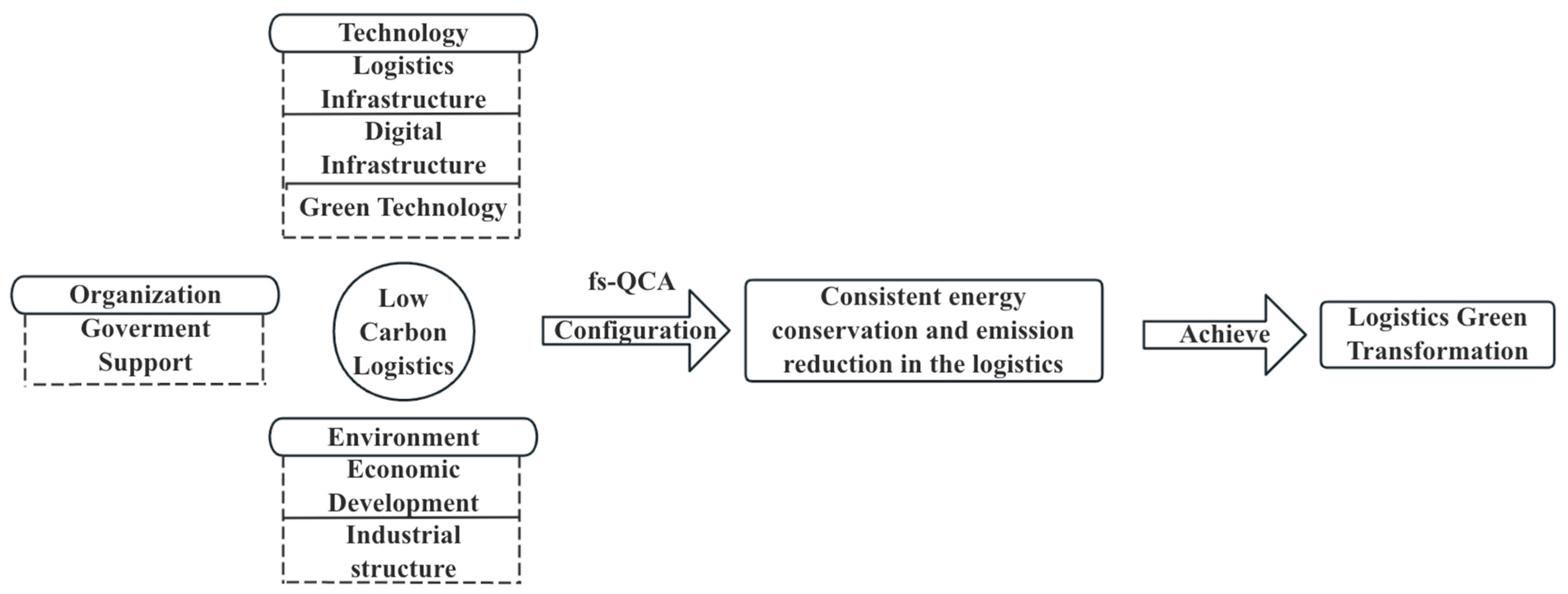
2. Theoretical Framework

In China’s traditional logistics industry, economic interests take precedence over environmental concerns. The logistics system is inherently complex, characterized by multiple inputs and outputs. However, previous studies have mainly employed linear or single-factor approaches, which fail to capture the complex interdependencies. Thus, based on Technology-Organization-Environment (TOE), we propose a configuration model to identify the key factors about the consistency of energy conservation and emission reduction in the logistics industry, as shown in Figure 1. This model serves as the foundation for the empirical design of the fs-QCA analysis in this study. The TOE framework integrates technological, organizational, and environmental factors to support sustainable development in the logistics sector. By applying fs-QCA, we identify multiple configurational pathways that promote sustainability in the logistics industry, thereby providing insights for its green transformation.

2.1. Technological Condition

Technological innovation plays a crucial role in promoting sustainable development within the logistics industry. Under the TOE framework, the integration and application of technology can effectively enhance logistics efficiency, thereby advancing sustainability objectives. The technological dimension includes logistics infrastructure (LI), digital infrastructure (DI), and green technology (GT). Robust infrastructure development enables enterprises to adopt collaborative logistics practices, such as road-to-rail shifts and multimodal transportation. These operations enhance overall logistics efficiency while reducing costs and pollutant emissions. The establishment of digital platforms integrates physical and digital systems, optimizes resource allocation, and enhances coordination among enterprises and transportation modes, ultimately reducing energy consumption. Investments in green technologies empower enterprises to adopt energy-saving technologies and clean energy solutions, transforming their energy use structure and promoting sustainable development.

2.2. Organizational Condition

The organizational dimension reflects the logistics industry’s ability to acquire and integrate external resources, particularly those provided by the government. As a key provider of external resources, the government plays a crucial role in accelerating the research, investment, and adoption of green technologies through policy measures such as financial support. Sufficient government funding demonstrates the government’s commitment to developing low-carbon logistics and its willingness to utilize fiscal resources to implement low-carbon logistics policies. This support directly accelerates the sustainable development of the logistics industry. Therefore, government support (GS) is treated as an organizational condition and is measured by the proportion of regional expenditures on energy conservation and emission reduction relative to total fiscal spending [28].

2.3. Environmental Condition

As a service industry, the variability of the external environment plays a crucial role in logistics demand, the service model, and the sustainable development of the logistics industry. The environmental dimension includes economic development (ED) and industrial structure (IS). Developed regions typically benefit from advanced infrastructure and mature economic environments, which make their logistics processes more flexible and facilitate the low-carbon transition of the logistics industry. From the perspective of the Environmental Kuznets Curve (EKC) [32], these regions prioritize the sustainable development of the logistics industry. On the other hand, developing regions at advancing past the beginning of the EKC focus on controlling costs and providing basic services, with environmental concerns being less important. This difference shows how regions along the EKC are at different stages in the development of their logistics industry. The GDP per capita serves as a direct indicator of economic development.

Industrial structure significantly shapes logistics demand and overall industry development. As industrial structures optimize and upgrade, production methods and technologies advance accordingly, leading to changes in logistics demand. The transition from traditional manufacturing to high-tech industries and the expansion of the service sector reshape logistics patterns, promoting more efficient and environmentally friendly logistics solutions. In regions dominated by heavy industries, logistics tends to focus on bulk transportation and raw material supply chains, whereas areas with a higher share of the tertiary industry require more advanced, service-oriented logistics solutions. The proportion of the tertiary industry’s output in total regional GDP is used as a core indicator for assessing IS.

3. Methodology

3.1. Theorems

Based on the production function theory proposed by Fare et al. [33], the following theorems are provided.

Theorem 1 

[29]. The production function with undesired outputs. This model represents the inputs (X) that produce the outputs (Y), while also yielding the undesired outputs (B), as follows.

$$P=\left\{\left(X,Y;B\right):X \mathrm{can} \mathrm{produce}\left(Y,B\right)\right\}$$

(1)

Theorem 1 indicates that undesired outputs are inherently produced alongside desired outputs during the production process.

Theorem 2 

[34]. The desired outputs and the undesired outputs exhibit weak disposability, as follows.

$$\mathrm{If}\left(X,Y;B\right)\in P \mathrm{and} 0\le \theta \le 1, \mathrm{then} \left(X,\theta Y;\theta B\right)\in P$$

(2)

Theorem 2 reflects that reducing undesirable outputs unavoidably leads to a reduction in desirable outputs, implying that emission reduction comes with an associated economic cost.

Theorem 3 

[30]. There is a null jointness between the desired outputs and the undesired outputs, as follows.

$$\mathrm{If}\left(X,Y;B\right)\in P \mathrm{and} B=0, \mathrm{then} Y=0$$

(3)

Theorem 3 indicates that desirable and undesirable outputs are jointly produced. Without the undesired outputs, there would be no desired outputs.

Definition 1. 

ECERE is used to measure the overall logistics efficiency, reflecting the integrated performance of energy conservation and emission reduction for each Decision-Making Unit (DMU); the formula is shown as follows.

$$ECERE=1-Non-ECERE$$

(4)

In the formula above, Non-ECERE represents the actual measured value by NDDF. ECERE directly reflects the sustainability of the logistics industry during its green transformation [26]. A value of ECERE approaching 1 indicates limited room for further improvement in energy conservation and emission reduction. When ECERE = 1, the DMU has achieved optimal green efficiency.

Definition 2. 

Cons represent the degree of consistency between energy conservation and emission reduction, with the formula shown as follows.

$$Cons=1-\left(ECE-ERE\right)$$

(5)

In Definition 2, the Cons value ranges from 0 to 1, where a value of 1 indicates consistency between ECE and ERE.

Definition 3 

[35]. Kernel density estimation is a non-parametric method used to estimate the probability density function of a random variable. Based on a finite data sample, it applies a Gaussian kernel to weight each data point, thereby revealing the dynamic temporal evolution of energy conservation and emission reduction efficiency. The formula is shown as follows.

$$p_n\left(x\right)={\displaystyle \frac{1}{nh}}{\displaystyle {\sum }_{i=1}^n\phi \left(\frac{x-x_i}{h}\right)}$$

(6)

In Definition 3, p_n(x) is the probability density estimate at point x, n is the number of samples, x_i is the sample point, $\phi$ is the Gaussian kernel function, and h is the bandwidth.

3.2. Data Source

Data were collected from 30 regions in China covering the period from 2011 to 2021 (due to the lack of data, the analysis of Xizang, Hong Kong, Macao, and Taiwan is not included). The data sources include the China Fiscal Yearbook, China Environmental Statistics Yearbook, China Tertiary Industry Statistics Yearbook, and the China Research Data Service Platform. The selection of study regions aligns with previous logistics efficiency research, and the sample size of 30 provinces meets the methodological requirements for this analysis [21,36]. The input variables selected to represent the logistics industry are fixed asset investment (K), number of employees (L), and total energy consumption (E). The desired outputs are industrial output value (V) and freight volume (F), while the undesired output is the total carbon emissions (C) from the logistics industry. The energy types include raw coal, gasoline, kerosene, diesel, fuel oil, liquefied petroleum gas, natural gas, and electricity. These energy sources are converted to standard coal based on reference factors and categorized into solid, liquid, and gaseous forms. Reference factors for the conversion of standard coal are shown in

Table 2. Standard coal conversion coefficients and carbon Emission factors.

Energy	Discount Factor for Standard Coal	Unit	Carbon Emission Factor	Unit
Raw coal	0.7143	Million tons of standard coal/million tons	0.7558	Tons of carbon/ton of standard coal
Gasoline	1.4714		0.5538
Kerosene	1.4714		0.5714
Diesel	1.4517		0.5821
Fuel oil	1.4286		0.6185
Liquefied petroleum gas	1.7143		0.5042
Natural gas	13.3	Million tons of standard coal/billion cubic meters	0.4483
Power	1.229	Million tons of standard coal/million kilowatt hours	2.2132

. Given that China relies primarily on coal for electricity generation, electricity is classified as a solid form of energy. Following Shan et al. and Guo et al. [37,38], carbon emissions are calculated using the methodology provided in the 2006 IPCC Guidelines, as shown in the following formula.

$$CE={\displaystyle \sum _{i=1}^{8}A{D}_i\times NC{V}_i}\times O_i\times C{C}_i=A{D}_i\times E{F}_i$$

(7)

where CE denotes the total carbon emissions, and i represents the type of energy. AD_i, NCV_i, O_i, and CC_i represent the consumption of fuel i, its net calorific value, the oxidation rate in the logistics industry, and the carbon content per unit of net calorific value, respectively. The product of the latter three parameters constitutes the carbon emission factor EF_i. The calculated values of EF are presented in Table 2.

The descriptive statistics of the input–output data are presented in

Table 3. Descriptive statistics of the input–output data.

	Indicator/Unit	OBS	Max	Min	Mean
Input	Fixed asset investment/100 million yuan	330	5386.95	100.3	5286.65
	Number of employees/10 thousand people	330	64.17	2.78	61.39
	Energy consumption /ten thousand tons of standard coal	330	3549.37	122.57	3426.8
Output	Industrial output value/100 million yuan	330	4166.8	67.53	4099.27
	Freight volume /ten thousand tons	330	434,298	12,586	421,712
	Carbon emissions /ten thousand tons	330	2357.05	78.3	2278.75

.

3.3. Efficiency Measurement Model

In accordance with Theorems 1–3, the direction vector can be expressed as g = (0,0,-E_j,0,0,-C), which indicates a reduction in energy input and carbon emissions. Based on the NDDF model, the energy structure model is as follows.

$$F1 \left\{\begin{array}{l} Non-ECERE=max\left[{\displaystyle \frac{1}{2}}({\displaystyle \sum _{j=1}^1\frac{1}{J}}{\omega }_{E_j}{\theta }_{E_t^j}+{\theta }_{C_t})\right]\\ s.t.{\displaystyle \sum _{n=1}^N{\lambda }_n}{K}_n\le K\\ {\displaystyle \sum _{n=1}^N{\lambda }_n}{L}_n\le L\\ {\displaystyle \sum _{n=1}^N{\lambda }_n}{E}_j\le E_j-{\theta }_{E_j}{g}_{E_j},j=1,2,\dots ,\left|\left.J\right|\right.\\ {\displaystyle \sum _{n=1}^N{\lambda }_n}{V}_n\ge V\\ {\displaystyle \sum _{n=1}^N{\lambda }_n}{F}_n\ge F\\ {\displaystyle \sum _{n=1}^N{\lambda }_n}{C}_n=C_n-{\theta }_C{g}_c\\ {\lambda }_n\ge 0, n=1,2,\dots ,N \\ {\theta }_{E_t^j},{\theta }_{C_t}\ge 0,j=1,2,\dots ,\left|\left.J\right|\right.\end{array}\right.$$

(8)

where θ represents the proportionate distance of the DMU from the production possibility frontier, ${\omega }_{E_j}=E_t^j/E_t$ is energy input weigh, $E_t^j$ represents the consumption of the j-the energy source in year t, $E_t$ is the total amount of energy consumed by the logistics industry in year t, J represents the type of energy input, λ links input and output variables to form a convex set, g specifies the direction of adjustment for inputs and outputs, T is the time period of measurement, and N is the number of province.

Given substitutability among input factors, it is necessary to treat capital and labor separately from energy inputs in the efficiency evaluation. The non-energy inputs and desirable outputs are assigned zero weights. This ensures the model captures the actual potential for energy conservation and emissions reduction. Meanwhile, assigning equal weights to inputs and outputs reflects a balanced evaluation framework that avoids bias toward either dimension. Based on the constructed model F1, four cases are obtained as follows.

M1: Consider the type of energy input, rather than the proportion of input. The direction vector is g = (0,0,-g_E1,-g_E2,-g_E3,0,0,-g_C), with weights ω = (0,0,1/3,1/3,1/3,0,0,1). The three types of energy inputs have equal weights.

M2: Consider both the type and proportion of energy inputs. Calculate the integrated compressibility ratio of energy input and carbon emissions. The direction vector is g = (0,0,-g_E1,-g_E2,-g_E3,0,0,-g_C), with weights ω = (0,0,ω_E1,ω_E2,ω_E3,0,0,1). The three types of energy inputs have equal proportions, and the weights are calculated using the energy structure formula ${\omega }_{E_j}=E_t^j/E_t$.

M3: Calculate the ratio of energy input that can be integrated, which value is ECE. The direction vector is g = (0,0,-g_E1,-g_E2,-g_E3,0,0,0), with weights ω = (0,0,2ω_E1,2ω_E2,2ω_E3,0,0,0). The energy input weights remain consistent with M2, and the carbon emission weight is set to 0.

M4: Calculate the ratio of carbon emissions that can be integrated; this value is referred to as ERE. The direction vector is g = (0,0,0,0,0,0,0,-g_C), with weights ω = (0,0,0,0,0,0,0,2). The carbon emission weight is set to 2, with no consideration of energy input.

4. Results

4.1. Comparison of Efficiency Measurement Models

The results of the calculation of M1 and M2 are shown in

Table 4. Result of M1 and M2.

Region	2011		2012		2013		2014		2015		2016
	M1	M2	M1	M2	M1	M2	M1	M2	M1	M2	M1	M2
Beijing	0.46	0.47	0.37	0.35	0.55	0.55	0.49	0.43	1	1	1	1
Tianjin	1	1	1	1	1	1	0.7	0.65	0.73	0.68	0.76	0.75
Hebei	1	1	1	1	1	1	1	1	1	1	1	1
Shanxi	0.46	0.52	0.49	0.56	0.47	0.53	0.47	0.52	0.62	0.75	0.71	0.86
Inner Mongolia	0.45	0.45	0.5	0.48	0.63	0.69	0.59	0.71	0.56	0.72	1	1
Liaoning	1	1	1	1	0.68	0.71	0.64	0.54	1	1	1	1
Jilin	0.39	0.44	0.42	0.44	1	1	1	1	1	1	1	1
Heilongjiang	0.37	0.36	0.38	0.33	0.39	0.33	0.32	0.28	0.33	0.29	0.37	0.37
Shanghai	1	1	1	1	1	1	1	1	1	1	1	1
Jiangsu	1	1	1	1	1	1	1	1	1	1	1	1
Zhejiang	1	1	1	1	1	1	1	1	1	1	1	1
Anhui	1	1	1	1	1	1	1	1	1	1	1	1
Fujian	0.79	0.78	1	1	1	1	1	1	1	1	1	1
Jiangxi	0.78	0.84	0.88	0.93	1	1	0.91	0.88	0.77	0.68	0.84	0.79
Shandong	1	1	1	1	0.83	0.76	0.86	0.79	0.77	0.68	0.82	0.74
Henan	0.67	0.64	0.75	0.73	0.66	0.72	0.71	0.72	0.6	0.57	0.62	0.64
Hubei	0.29	0.35	0.32	0.37	0.45	0.42	0.43	0.4	0.46	0.44	0.45	0.41
Hunan	0.9	0.92	1	1	0.69	0.66	0.64	0.59	0.65	0.61	0.67	0.65
Guangdong	0.57	0.49	0.6	0.53	0.72	0.66	0.78	0.7	0.9	0.86	1	1
Guangxi	1	1	1	1	1	1	1	1	1	1	1	1
Hainan	1	1	0.5	0.43	0.47	0.41	1	1	0.56	0.5	0.54	0.49
Chongqing	0.53	0.5	0.44	0.45	0.47	0.46	0.6	0.6	0.59	0.58	0.6	0.6
Sichuan	0.58	0.53	0.61	0.57	0.7	0.7	0.66	0.66	0.75	0.79	0.67	0.67
Guizhou	1	1	1	1	1	1	1	1	1	1	1	1
Yunnan	0.37	0.42	0.42	0.47	0.73	0.8	0.66	0.73	0.68	0.76	0.68	0.74
Shaanxi	0.35	0.36	0.4	0.43	0.52	0.53	0.54	0.53	0.57	0.59	0.69	0.72
Gansu	0.35	0.4	0.4	0.42	0.31	0.3	0.3	0.3	0.33	0.36	0.34	0.4
Qinghai	0.32	0.34	0.32	0.36	0.31	0.34	0.32	0.33	0.34	0.38	0.34	0.37
Ningxia	1	1	1	1	1	1	0.61	0.66	0.68	0.75	0.72	0.77
Xinjiang	0.31	0.32	0.34	0.36	0.3	0.32	0.31	0.33	0.29	0.31	0.32	0.34
Region	2017		2018			2019		2020		2021
	M1	M2	M1	M2		M1	M2	M1	M2	M1	M2
Beijing	0.72	0.61	0.44	0.33		0.44	0.72	0.61	0.44	0.33	0.44
Tianjin	1	1	1	1		0.8	1	1	1	1	0.8
Hebei	1	1	1	1		1	1	1	1	1	1
Shanxi	1	1	1	1		1	1	1	1	1	1
Inner Mongolia	1	1	1	1		1	1	1	1	1	1
Liaoning	1	1	1	1		1	1	1	1	1	1
Jilin	0.58	0.61	0.47	0.44		0.45	0.58	0.61	0.47	0.44	0.45
Heilongjiang	0.35	0.35	0.25	0.24		0.22	0.35	0.35	0.25	0.24	0.22
Shanghai	1	1	1	1		1	1	1	1	1	1
Jiangsu	1	1	0.74	0.71		0.73	1	1	0.74	0.71	0.73
Zhejiang	1	1	1	1		1	1	1	1	1	1
Anhui	1	1	1	1		1	1	1	1	1	1
Fujian	1	1	1	1		1	1	1	1	1	1
Jiangxi	1	1	1	1		1	1	1	1	1	1
Shandong	0.85	0.79	0.88	0.82		1	0.85	0.79	0.88	0.82	1
Henan	0.56	0.57	0.94	0.96		0.99	0.56	0.57	0.94	0.96	0.99
Hubei	0.46	0.41	0.59	0.5		0.63	0.46	0.41	0.59	0.5	0.63
Hunan	0.66	0.67	0.52	0.51		0.54	0.66	0.67	0.52	0.51	0.54
Guangdong	0.91	0.87	0.61	0.49		0.65	0.91	0.87	0.61	0.49	0.65
Guangxi	1	1	0.48	0.5		0.54	1	1	0.48	0.5	0.54
Hainan	0.56	0.5	0.59	0.45		0.75	0.56	0.5	0.59	0.45	0.75
Chongqing	0.6	0.57	0.57	0.52		0.57	0.6	0.57	0.57	0.52	0.57
Sichuan	0.65	0.64	0.56	0.47		0.58	0.65	0.64	0.56	0.47	0.58
Guizhou	1	1	0.6	0.5		0.57	1	1	0.6	0.5	0.57
Yunnan	0.7	0.74	0.66	0.7		0.6	0.7	0.74	0.66	0.7	0.6
Shaanxi	0.69	0.72	0.61	0.65		0.62	0.69	0.72	0.61	0.65	0.62
Gansu	0.33	0.39	0.35	0.42		0.35	0.33	0.39	0.35	0.42	0.35
Qinghai	0.31	0.32	0.28	0.29		0.26	0.31	0.32	0.28	0.29	0.26
Ningxia	0.65	0.64	0.52	0.61		1	0.65	0.64	0.52	0.61	1
Xinjiang	0.34	0.33	0.35	0.34		0.45	0.34	0.33	0.35	0.34	0.45

. Table 4 shows that the efficiency values for M1 ranged from 0.643 to 0.771, while those for M2 ranged from 0.624 to 0.777. In most years, M1 showed higher efficiency than M2. When equal weight was assigned to energy input, logistics efficiency appeared higher. This highlights that reducing the proportion of oil energy, increasing the use of clean energy sources such as natural gas, and balancing the energy input structure can effectively enhance logistics efficiency. The eastern regions exhibited higher efficiency values compared to the western provinces. In the eastern regions, Hebei, Shanghai, and Anhui consistently maintained efficiency values of 1 throughout the measurement period. Jiangsu, Zhejiang, and Fujian had average efficiency values above 0.9, reflecting their strong performance. In contrast, the western regions showed more fluctuation, with generally lower efficiency levels.

From a temporal perspective, the average efficiency for M2 increased from 0.704 in 2011 to 0.777 in 2017, before declining to 0.624 in 2020, and then rebounding in 2021. This fluctuation aligns with Porter’s theory, which indicates that while stringent environmental regulations may initially reduce industrial efficiency, they can also drive innovation in clean technologies and processes. The decline in efficiency in 2020 corresponds with the low-carbon targets set by the 13th Five-Year Plan for energy conservation and environmental protection in transportation. The rebound in 2021 reflects the positive long-term effects of these policies.

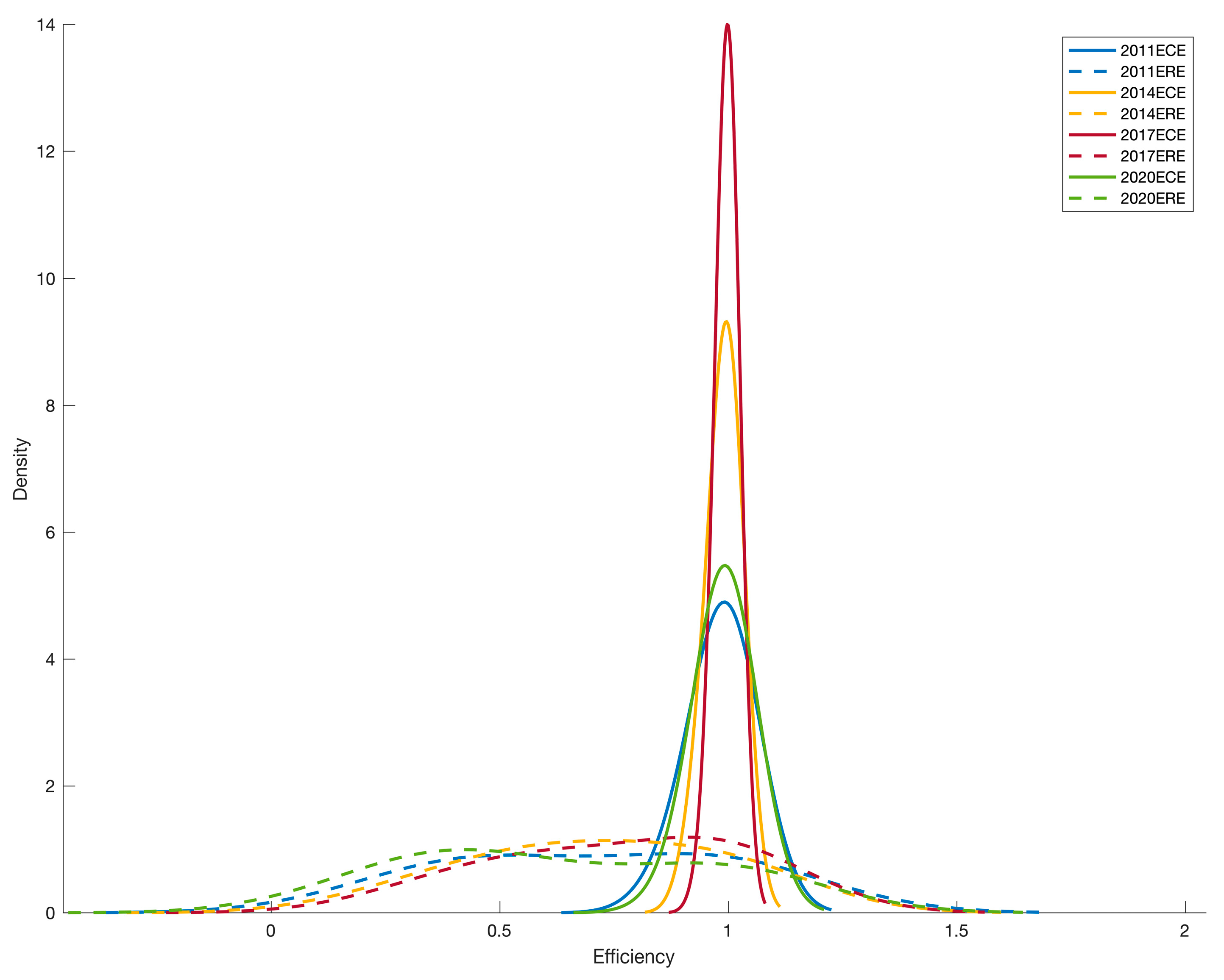
4.2. Measurement and Analysis of the ECE and ERE

The ECE and ERE were calculated, and the results are shown in Figure 2, where the blue line represents ECE and the red line represents ERE. When the two points overlap, it means that ECE and ERE have reached consistency. The fluctuation patterns can be categorized into four distinct types: (a) shows a steady upward trend, (b) is a gradual downward trend, (c) shows stable low-level performance, and (d) shows mixed dynamics. According to the measurement results, the ECE is effective in 258 of the DMUs, with the lowest value of 0.87 observed in Heilongjiang in 2020. The ERE is only effective in 127 DMUs.

From a spatial perspective, notable regional disparities exist across the eastern, central, and western regions (according to the division of the three major economic regions, the eastern region includes Beijing, Tianjin, Hebei, Liaoning, Shanghai, Jiangsu, Zhejiang, Fujian, Shandong, Guangdong, Guangxi, and Hainan; the central region includes Shanxi, Inner Mongolia, Jilin, Heilongjiang, Anhui, Jiangxi, Henan, Hubei, and Hunan; the western region includes Chongqing, Sichuan, Guizhou, Yunnan, Shaanxi, Gansu, Ningxia, Qinghai, and Xinjiang). A significant gap exists between the eastern and western regions. In the eastern region, 60% of DMUs achieved consistency between ECE and ERE. In the central region, 34% of DMUs achieved consistency. In the western region, only 13% of DMUs achieved consistency.

From a temporal perspective, the panel data for the measurement period are divided into 2011, 2014, 2017, and 2020. Using Formula (6), the kernel density values are calculated as shown in Figure 3. In the figure, the solid line is ECE, the dashed line is ERE, and the kernel density values for 2011, 2014, 2017, and 2020 are represented by blue, yellow, red, and green, respectively. The x-axis represents efficiency values, while the y-axis denotes probability density. A higher probability density indicates a greater concentration of data points near the peak of the curve. The width of the curve reflects the dispersion of the data, with a wider curve indicating a greater dispersion degree. Figure 3 indicates that ECE values are consistently higher than those of the ERE across all time periods. The kernel density of the ECE is concentrated around 1. By examining the kernel density peaks, we find that the ECE is clustered around 1, indicating an overall upward trend in regions with the ECE. Although the peak for ERE is less pronounced, the rightward shift of the curve implies a gradual enhancement in emission reduction performance.

In summary, the findings reveal a general inconsistency between ECE and ERE, with ECE generally higher than the ERE. The results show that emission reduction depends on energy conservation, but energy saving alone does not necessarily lead to emission reduction. Notably, when ECE and ERE are aligned, the result of M2 reaches 1. In order to achieve green, efficient, and sustainable development of the logistics industry, it is crucial to explore development pathways that ensure a high degree of consistency between energy conservation and emission reduction.

5. fs-QCA

5.1. Sample Selection

Based on data from 30 provinces in 2021, this section explores the configuration paths leading to high Cons. The conditional variables include logistics infrastructure (LI), digital infrastructure (DI), green technology (GT), government support (GS), economic development (ED), and industrial structure (IS).

5.2. Calibration

The direct calibration method [39,40] is applied to calibrate the six conditional variables and the outcome variable. According to the distribution of the sample data, the 75th percentile is set as the threshold for full membership, the 50th percentile as the crossover point, and the 25th percentile as the threshold for full non-membership. For cases where the membership score after calibration is 0.5, these scores are adjusted to 0.501. Detailed calibration thresholds are provided in

Table 5. Calibration anchors of each fuzzy set and descriptive statistics.

Sets	Calibration Anchors			Descriptive Analysis
	Fully In (75%)	Crossover (50%)	Fully Out (25%)	Min	Max	Mean
Cons	1	0.69	0.453	0.24	1	0.70
LI	13,957.44	11,638.82	7349.88	1247.23	24,030.33	11,218.92
DI	0.841	0.735	0.657	0.51	1.07	0.75
GT	5189	2650	1198	256	24,072	5092.36
GS	213.695	161.525	98.178	47.13	493.55	174.13
ED	86,763.25	65,592.5	58,117	41,046	183,980	80,537.3
IS	0.529	0.511	0.491	0.435	0.833	0.529

.

5.3. Analysis of Necessary Conditions

Necessity analysis provides an initial understanding of which conditions are essential. A condition is considered necessary if it consistently appears when the outcome occurs. The consistency in fs-QCA refers to the degree to which a condition or combination of conditions aligns with the outcome. If the consistency index exceeds the preset threshold (usually 0.9), the condition is considered necessary.

Table 6. Analysis results of necessary.

Conditions	Results
	High Cons		Low Cons
	Consistency	Coverage	Consistency	Coverage
LI	0.602007	0.579151	0.520266	0.503861
~LI	0.484281	0.500692	0.565448	0.58852
DI	0.551839	0.566621	0.505648	0.522665
~DI	0.535117	0.518135	0.580731	0.566062
GT	0.606154	0.581568	0.513621	0.496085
~GT	0.474783	0.492301	0.566777	0.591622
GS	0.553846	0.545455	0.569435	0.564559
~GS	0.55786	0.562753	0.541528	0.549932
ED	0.480334	0.474526	0.591495	0.588251
~ED	0.583211	0.586467	0.471628	0.477433
IS	0.58796	0.583665	0.487043	0.48672
~IS	0.482943	0.483266	0.583389	0.587684

Note: ~ represents a non-set of an antecedent condition.

presents the analysis of necessary conditions; none of the conditional variables meet this threshold, indicating that there are no necessary conditions.

5.4. Configuration Paths

The parameter settings are as follows: the case frequency threshold is set to 1, the original consistency threshold is set to 0.8, and the PRI threshold is set to 0.75. We assume that either the presence or absence of a single conditional factor may lead to high or low Cons. This result focuses on the intermediate and parsimonious solutions. Conditions appearing in both solutions are considered core conditions, while those that appear only in the intermediate solution are considered peripheral conditions. There are five identified paths to achieve high Cons, as detailed in

Table 7. Sufficient configurations.

Antecedent Condition	High Cons					Low Cons
	H1	H2	H3a	H3b	H4	NH1	NH2
LI	O	x		x	O	X
DI	O	o	x	x	x	o	X
GT	x	o	X	X	o	O	x
GS	x	X	o		O	o	X
ED	X	O	O	O	x	x	X
IS	o	X	X	X	X	O	X
Consistency	1	0.992958	0.915085	0.912664	0.859922	0.967033	0.94471
Raw coverage	0.0668896	0.0943144	0.122542	0.125819	0.147826	0.0584718	0.249767
Unique coverage	0.0474916	0.0548495	0.0234782	0.0214047	0.10301	0.0431894	0.234485
Over solution consistency	0.933583					0.946341
Over solution coverage	0.366689					0.292957

Note: O and X = core causal condition (present/absent). o and x = contributing causal condition (present/absent). Blank spaces indicate a do not care condition.

, where O represent the presence of conditions and X represent their absence. Larger symbols represent core conditions, while smaller symbols represent auxiliary conditions.

H1 is an infrastructure-driven configuration path. Along with an industry structure becoming tertiary-based, regions with high levels of LI and DI can still achieve high Cons, even if GT, GS, and ED are relatively low. A typical province exemplifying this configuration is Hainan. Hainan has optimized the comprehensive transport layout and strengthened multimodal transport capabilities in LI. In terms of DI, the province has actively promoted the integration of new-generation information technologies with its economic and social development, in line with the Smart Hainan General Plan in 2020. Although green innovation remains somewhat insufficient, the integration technologies of big data, the IoT, and artificial intelligence in smart logistics, intelligent transportation, and digital supply chain systems have significantly improved logistics energy efficiency and reduced carbon emissions.

H2 is the digital economy-driven configuration path. In regions following the H2 path, high levels of ED, DI, and GT lead to high Cons, while low levels of GS and IS are core absent conditions. Fujian is a representative case of this path. Its strong economic foundation enables substantial investment in DI and GT. DI offers a technological platform to accelerate GT, forming a positive feedback mechanism among the three. Fujian’s logistics market is mature and mainly driven by market dynamics and self-innovation rather than direct government financial support. Logistics companies promote the adoption of green technologies through internal R&D, external investment, or market-driven forces. The logistics industry then forms a service system that effectively combines internal and external resources to advance the sustainable development of logistics.

H3a and H3b represent the industrial economy-driven configuration path. In H3a and H3b, LI and GS serve as substitutes, with both sharing the same core conditions. Compared to H2, these paths do not rely on digital or green technological capabilities, while ED and IS remain as common core conditions. Shanxi and Inner Mongolia are typical cases. These provinces are key resource bases in China, where the economy largely relies on the secondary industry. In 2020, Inner Mongolia increased its investment in environmental protection by 23.2%. Its 13th Five-Year Energy Development Plan has spurred clean energy growth by raising wind and solar power’s share while reducing fossil fuel reliance, which makes it the largest new energy production area in China. Overall, this path shows that an industrial economy-driven model can transform energy structures, protect the environment, and promote the sustainable development of the logistics industry.

H4 is the government support-driven configuration path. In this configuration, high levels of GS and GT, often accompanied by robust LI, are key to achieving high Cons. A typical case is Henan Province, which boasts a well-developed logistics infrastructure, with six cities and ten logistics hubs included in the National Logistics Hub Layout and Construction Plan. Henan has accelerated the adoption of green technologies in logistics infrastructure, enhancing energy conservation and emission reduction. By promoting multimodal integration across air, water, road, and rail networks, the province has improved coordination and operational efficiency. Continuous government investment has facilitated the widespread adoption of green technologies in logistics and transportation. For instance, Henan actively funds research and promotes new energy vehicles, optimizing the transport structure and lowering emissions, thereby advancing the sustainable transformation of the logistics sector.

There are two low Cons paths: NH1, represented by Sichuan, and NH2, represented by Heilongjiang, Yunnan, and Guizhou. The two paths show clear differences. In the NH1 path, several conditions are at a high level, but LI is a core absent condition. Although GT and DI are relatively advanced, the lack of foundational infrastructure appears to constrain logistics development, undermining the overall efficiency. In the NH2 path, multiple conditions are core absent factors. In these regions, insufficient economic capacity limits government support, while technological deficiencies hinder the development of sustainable logistics systems. In this context, high Cons cannot be realized, regardless of the state of logistics infrastructure.

5.5. Robust Analysis

A robustness test was conducted to examine whether the fs-QCA results exhibited significant alterations in response to distinct operational choices. The test involved adjusting the case frequency, PRI consistency, and calibration anchor points. Increasing the case frequency makes the findings more conservative, ensuring that only well-supported configurations are retained. Conversely, lowering PRI consistency includes more causal paths, and variations in calibration thresholds influence the final configuration path. First, the case frequency was adjusted from 1 to 2, resulting in configurations that were largely consistent with the existing solutions. Second, the PRI consistency was increased to 0.8 and decreased to 0.7, and the resulting configurations still largely encompassed the existing ones. Finally, the intersection anchor points of the conditional variables were adjusted to 85%, 50%, and 15%, and remained basically consistent with the existing findings; the results are shown in

Table 8. Robust analysis.

Antecedent Condition	High Cons			Low Cons
	H1	H2	H3a	NH1	NH2
LI	x	X	O	X
DI	o	x	x	o	x
GT	o	x	o	O	x
GS	X		O	o	X
ED	O	O	x	x	X
IS	X	x	X	O	X
Consistency	0.891213	0.84326	0.806201	0.901709	0.802594
Raw coverage	0.139856	0.176625	0.204859	0.153232	0.404502
Unique coverage	0.0216678	0.0630336	0.133946	0.0341322	0.289034
Over solution consistency	0.828756			0.779176
Over solution coverage	0.336835			0.494553

Note: O and X = core causal condition (present/absent). o and x = contributing causal condition (present/absent). Blank spaces indicate a do not care condition.

. These findings confirm the robustness of the original fs-QCA results across different analytical settings.

6. Conclusions

6.1. Discussion of Results

(1)

The logistics industry exhibits distinctive characteristics in terms of energy conservation and emission reduction. From 2011 to 2021, the average M2 in the national logistics industry ranged between 0.624 and 0.777. Consistent with previous studies on provincial logistics efficiency in China, this paper finds that the eastern regions performed better than the central and western regions. Earlier studies integrated energy conservation and emission reduction into logistics efficiency as a single concept. In contrast, this paper differentiates between ECE and ERE. The ECE and ERE are expected to be consistent. However, calculations reveal a discrepancy between them. In general, the ECE was higher than the ERE. The ECE and ERE were aligned in only 129 of the 330 DMUs. The findings suggest that logistics efficiency reaches its optimal level when ECE and ERE are consistent.

(2)

Based on the fs-QCA analysis, this study identifies four distinct development pathways leading to consistent energy conservation and emission reduction in the logistics industry. The four high Cons configuration paths covered 36.6% of the cases. These high Cons configurations reflect the joint effects of key conditions such as transportation infrastructure, government support, green technology innovation, and digital development.

(3)

Two low Cons configuration paths were identified, covering 29.2% of the cases, predominantly located in the western regions. The NH1 suggests that even with technological advancement, the lack of basic infrastructure significantly constrains the efficiency and sustainability of logistics operations. NH2 shows that multiple core conditions are absent, and the development of sustainable logistics is severely hampered, regardless of the status of logistics infrastructure. Therefore, building a consistent development system for the ECE and the ERE in the logistics industry requires the coordinated promotion of multiple factors.

(4)

Despite the valuable insights provided by this study, several limitations remain. First, while it analyzes the impact of energy structure changes on logistics efficiency from a macro perspective, it does not provide precise quantitative values for specific energy structure adjustments. Second, although the fs-QCA provides valuable insights into different pathways for improving green logistics efficiency, its results are highly dependent on the selection of conditions and thresholds.

6.2. Managerial Implications

(1)

Regions classified as H1 refer to those with well-developed logistics infrastructure and digital capabilities. To achieve sustainable development, it is imperative for these regions to deepen the integration between digital ecosystems and physical infrastructure systems. Cloud computing, artificial intelligence, and blockchain technologies should be applied to develop collaborative platforms that strengthen the coordination between digital infrastructure and logistics operations. By coupling virtual and physical systems, digital twin models can be formed to enhance real-time supervision, improve energy efficiency, and reduce carbon emissions.

(2)

Regions classified as H2 and H4 refer to those with strong digital capabilities and high levels of economic development. These regions are at the forefront of the digital economy and could drive the large-scale application of green and low-carbon technologies in the logistics sector. By embedding green technologies into digital platforms and strengthening data connectivity across logistics nodes, they can enhance supply chain transparency and coordination. This facilitates the integration of upstream and downstream industries, laying the groundwork for a collaborative and low-carbon logistics ecosystem.

(3)

Regions classified as H3a and H3b refer to those driven by secondary industry. In these areas, accelerating the use of clean energy to replace fossil fuels in industrial production and transportation is key to reducing carbon emissions. As energy structures shift, logistics activities such as procurement, distribution, and delivery also become greener. Meanwhile, the integration of production-oriented services enables more precise supply chain coordination and resource efficiency, gradually forming a sustainable development model through the synergy of the secondary and tertiary sectors.

References

1. LogClub. China Green Logistics Development Report. [EB/OL]. Available online: https://www.logclub.com/front/lc_report/get_report_info/3977 (accessed on 12 March 2023).
2. CEIC China Energy: Final Consumption: Transport, Storage, Postal & Telecom Service. [EB/OL]. Available online: https://www.ceicdata.com.cn/zh-hans/china/energy-balance-sheet/cn-energy-final-consumption-transport-storage-postal--telecom-service (accessed on 5 September 2024).
3. Zeng, S.; Su, B.; Zhang, M.; Gao, Y.; Liu, J.; Luo, S.; Tao, Q. Analysis and forecast of China’s energy consumption structure. Energy Policy 2021, 159, 112630. [Google Scholar] [CrossRef]
4. Liang, H.; Lin, S.; Wang, J. Impact of technological innovation on carbon emissions in China’s logistics industry: Based on the rebound effect. J. Clean. Prod. 2022, 377, 134371. [Google Scholar] [CrossRef]
5. Wang, Q.; Su, B.; Sun, J.; Zhou, P.; Zhou, D. Measurement and decomposition of energy-saving and emissions reduction performance in Chinese cities. Appl. Energy 2015, 151, 85–92. [Google Scholar] [CrossRef]
6. Barma, M.C.; Saidur, R.; Rahman, S.M.A.; Allouhi, A.; Akash, B.A.; Sait, S.M. A review on boilers energy use, energy savings, and emissions reductions. Renew. Sustain. Energy Rev. 2017, 79, 970–983. [Google Scholar] [CrossRef]
7. Jimenez, V.J.; Kim, H.; Munim, Z.H. A review of ship energy efficiency research and directions towards emission reduction in the maritime industry. J. Clean. Prod. 2022, 366, 132888. [Google Scholar] [CrossRef]
8. Li, X.; Xu, H. The energy-conservation and emission-reduction paths of industrial sectors: Evidence from Chinas 35 industrial sectors. Energy Econ. 2020, 86, 104628. [Google Scholar] [CrossRef]
9. Markovits-Somogyi, R.; Bokor, Z. Assessing the logistics efficiency of European countries by using the DEA-PC methodology. Transport 2014, 29, 137–145. [Google Scholar] [CrossRef]
10. Zheng, W.; Xu, X.; Wang, H. Regional logistics efficiency and performance in China along the Belt and Road Initiative: The analysis of integrated DEA and hierarchical regression with carbon constraint. J. Clean. Prod. 2020, 276, 123649. [Google Scholar] [CrossRef]
11. Yang, W.; Liu, D.; Sui, X.; Li, F. Does logistics efficiency matter? Evidence from green economic efficiency side. Res. Int. Bus. Financ. 2022, 61, 101650. [Google Scholar]
12. Khan, S.A.R.; Qianli, D. Does national scale economic and environmental indicators spur logistics performance? Evidence from UK. Environ. Sci. Pollut. Res. 2017, 24, 26692–26705. [Google Scholar] [CrossRef]
13. Park, Y.S.; Lim, S.H.; Egilmez, G.; Szmerekovsky, J. Environmental efficiency assessment of US transport sector: A slack-based data envelopment analysis approach. Transp. Res. Part D Transp. Environ. 2018, 61, 152–164. [Google Scholar] [CrossRef]
14. Lo Storto, C.; Evangelista, P. Infrastructure efficiency, logistics quality and environmental impact of land logistics systems in the EU: A DEA-based dynamic mapping. Res. Transp. Bus. Manag. 2023, 46, 100814. [Google Scholar] [CrossRef]
15. Zhou, P.; Ang, B.W.; Wang, H. Energy and CO2 emission performance in electricity generation: A non-radial directional distance function approach. Eur. J. Oper. Res. 2012, 221, 625–635. [Google Scholar] [CrossRef]
16. Dakpo, K.H.; Jeanneaux, P.; Latruffe, L. Modelling pollution-generating technologies in performance benchmarking: Recent developments, limits and future prospects in the nonparametric framework. Eur. J. Oper. Res. 2016, 250, 347–359. [Google Scholar] [CrossRef]
17. Yao, X.; Cheng, Y.; Zhou, L.; Song, M. Green efficiency performance analysis of the logistics industry in China: Based on a kind of machine learning methods. Ann. Oper. Res. 2020, 308, 727–752. [Google Scholar] [CrossRef]
18. Qin, W.; Qi, X. Evaluation of Green Logistics Efficiency in Northwest China. Sustainability 2022, 14, 6848. [Google Scholar] [CrossRef]
19. Liang, Z.J.; Chiu, Y.H.; Guo, Q.; Liang, Z. Low-carbon logistics efficiency: Analysis on the statistical data of the logistics industry of 13 cities in Jiangsu Province, China. Res. Transp. Bus. Manag. 2022, 43, 100740. [Google Scholar] [CrossRef]
20. Lu, M.; Lei, W.; Gao, Y.; Wan, Q. If There Appears a Path to Improve Chinese Logistics Industry Efficiency in Low-Carbon Perspective? A Qualitative Comparative Analysis of Provincial Data. Math. Probl. Eng. 2021, 2021, 9977497. [Google Scholar] [CrossRef]
21. Chen, B.; Liu, F.; Gao, Y.; Ye, C. Spatial and temporal evolution of green logistics efficiency in China and analysis of its motivation. Environ. Dev. Sustain. 2024, 26, 2743–2774. [Google Scholar] [CrossRef]
22. Xin, Y.; Zheng, K.; Zhou, Y.; Han, Y.; Tadikamalla, P.R.; Fan, Q. Logistics efficiency under carbon constraints based on a super SBM model with undesirable output: Empirical evidence from China’s logistics industry. Sustainability 2022, 14, 5142. [Google Scholar] [CrossRef]
23. Zhang, J.; Chang, Y.; Wang, C.; Zhang, L. The green efficiency of industrial sectors in China: A comparative analysis based on sectoral and supply-chain quantifications. Resour. Conserv. Recycl. 2018, 132, 269–277. [Google Scholar] [CrossRef]
24. Guo, X.; Li, B. Efficiency evaluation of regional logistics industry and its influencing factors under low-carbon constraints. Environ. Dev. Sustain. 2024, 26, 15667–15679. [Google Scholar] [CrossRef]
25. Lu, M.; Xie, R.; Chen, P.; Zou, Y.; Tang, J. Green transportation and logistics performance: An improved composite index. Sustainability 2019, 11, 2976. [Google Scholar] [CrossRef]
26. Ye, C.; Huang, Z.X.; Wei, J.; Wang, X. Spatial-Temporal Evolutionary Characteristics and Its Driving Mechanisms of China’s Logistics Industry Efficiency under Low Carbon Constraints. Pol. J. Environ. Stud. 2022, 31, 5405–5417. [Google Scholar] [CrossRef] [PubMed]
27. Li, M.; Huang, K.; Xie, X.; Chen, Y. Dynamic evolution, regional differences and influencing factors of high-quality development of China’s logistics industry. Ecol. Indic. 2024, 159, 111728. [Google Scholar] [CrossRef]
28. Qin, W. Spatial-temporal Evolution and Improvement Path of Logistics Industry Efficiency in Guangdong-Hong Kong-Macao Greater Bay Area. China Bus. Mark. 2020, 34, 31–40. [Google Scholar] [CrossRef]
29. Gong, X. Measurement of regional logistics efficiency and analysis of influencing factors. Stat. Decis. 2022, 38, 112–116. [Google Scholar] [CrossRef]
30. Fiss, P.C. Building better causal theories: A fuzzy set approach to typologies in organization research. Acad. Manag. J. 2011, 54, 393–420. [Google Scholar] [CrossRef]
31. Greckhamer, T.; Furnari, S.; Fiss, P.C.; Aguilera, R.V. Studying configurations with qualitative comparative analysis: Best practices in strategy and organization research. Strateg. Organ. 2018, 16, 482–495. [Google Scholar] [CrossRef]
32. Grossman, G.M.; Krueger, A.B. Economic growth and the environment. Q. J. Econ. 1995, 110, 353–377. [Google Scholar] [CrossRef]
33. Fare, R.; Grosskopf, S.; Pasurka, C.A. Enviromental production functions and enviromental Directional Distance Functions. Energy 2007, 32, 1055–1066. [Google Scholar] [CrossRef]
34. D’Inverno, G.; Carosi, L.; Romano, G.; Guerrini, A. Water pollution in wastewater treatment plants: An efficiency analysis with undesirable output. Eur. J. Oper. Res. 2018, 269, 24–34. [Google Scholar] [CrossRef]
35. Gramacki, A. Nonparametric Kernel Density Estimation and Its Computational Aspects; Springer International Publishing: Cham, Switzerland, 2018. [Google Scholar]
36. Zhang, H.; You, J.; Haiyirete, X.; Zhang, T. Measuring logistics efficiency in China considering technology heterogeneity and carbon emission through a meta-frontier model. Sustainability 2020, 12, 8157. [Google Scholar] [CrossRef]
37. Shan, Y.; Guan, D.; Liu, J.; Mi, Z.; Liu, Z.; Liu, J.; Schroeder, H.; Cai, B.; Chen, Y.; Shao, S.; et al. Methodology and applications of city level CO2 emission accounts in China. J. Clean. Prod. 2017, 161, 1215–1225. [Google Scholar] [CrossRef]
38. Guo, Z.; Tian, Y.; Guo, X.; He, Z. Research on measurement and application of China’s regional logistics development level under low carbon environment. Processes 2021, 9, 2273. [Google Scholar] [CrossRef]
39. Pappas, I.O.; Woodside, A.G. Fuzzy-set Qualitative Comparative Analysis (fsQCA): Guidelines for research practice in Information Systems and marketing. Int. J. Inf. Manag. 2021, 58, 102310. [Google Scholar] [CrossRef]
40. Khan, A.; Rezaei, S.; Valaei, N. Social commerce advertising avoidance and shopping cart abandonment: A fs/QCA analysis of German consumers. J. Retail. Consum. Serv. 2022, 67, 102976. [Google Scholar] [CrossRef]
Figure 1. Theoretical framework.
Sustainability 17 04629 g001
Figure 2. ECE and ERE in 30 provinces. (a) Steady upward trend. (b) Gradual downward trend. (c) Stable low-level performance. (d) Mixed dynamic.
Sustainability 17 04629 g002
Figure 3. ECE and ERE kernel density curve.
Sustainability 17 04629 g003