2. State of the Art
In recent years, research on bike-sharing systems has gained relevance due to their positive impact on sustainable urban mobility and their contribution to reducing traffic congestion. Recent research covers topics ranging from efficient bicycle distribution to identifying areas with low accessibility, highlighting how these factors influence the use and efficiency of such systems.
Ensuring that users have easy access to the city’s bike-sharing system is crucial for ensuring its usage and effectiveness, which, in turn, supports sustainable urban mobility. Studies have shown that accessibility plays a significant role in determining whether individuals choose to use these services. Each additional meter a user must walk to a station decreases their probability of using the service by 0.194% [
18]. This highlights the need for strategically placed stations to minimize walking distances and encourage participation. Similarly, a 10% increase in bicycle availability leads to a 12.21% rise in usage, emphasizing the importance of maintaining enough bicycles to meet demand. These findings underscore the necessity of identifying vulnerable areas and prioritizing infrastructure expansion to improve access and enhance overall mobility in the city.
Recent research has also focused on enhancing spatial analysis techniques to improve bike-sharing management. Geographic Information Systems (GIS) have been employed to evaluate station placement and accessibility. Studies such as [
19] have demonstrated how GIS-based methods can optimize station locations, considering factors like population density, urban morphology, and proximity to key services. Integrating spatial analysis allows for better identification of underserved areas and ensures a more equitable distribution of bicycles.
Managing peaks in demand is essential to prevent bicycle shortages or overcrowding at specific stations. Analyzing usage patterns enables cities to anticipate critical situations and optimize bike-sharing operations. Studies conducted in Chicago [
20] have applied time-series clustering techniques to identify trends in bike-sharing systems, offering valuable insights into demand fluctuations. Similarly, research in New York [
21] has utilized predictive models to forecast station-level demand, helping operators make informed decisions to improve availability and efficiency.
Based on these predictions, redistribution strategies can be implemented to optimize bicycle availability. Various dynamic models have been developed to optimize the redistribution of bicycles in bike-sharing systems, helping to maintain availability, improve efficiency and reduce costs. For example, one such model [
22] focuses on reducing repositioning costs while ensuring users can reliably find available bicycles and docking stations. Similarly, other approaches, such as the optimization model designed for Wuhan’s bicycle-sharing network [
23], have been designed to enhance large-scale bike-sharing systems, adapting to different urban environments and usage patterns.
Beyond operational redistribution using service vehicles, recent studies have explored user-based rebalancing strategies that leverage pricing incentives and gamification mechanisms to encourage users to reposition bicycles themselves. Research has demonstrated that offering discounts, extra ride time, or rewards can significantly influence user behavior, reducing the need for costly truck-based repositioning [
24,
25]. Dynamic pricing models [
26,
27] adjust trip costs based on current system imbalances, making it financially attractive for users to participate in rebalancing activities. These strategies not only lower operational costs but also promote a more environmentally sustainable system by minimizing vehicle emissions associated with traditional repositioning operations. However, despite their partial effectiveness in certain contexts, these methods do not always guarantee sufficient rebalancing, especially in situations of high demand or in areas with lower user appeal. Therefore, direct intervention through replenishment teams using trucks remains essential to ensure the system’s operability and availability throughout the city.
Moreover, sustainability assessments of bike-sharing systems are gaining attention through Life Cycle Assessment (LCA) methodologies. LCA provides a comprehensive evaluation of the environmental impacts associated with all stages of a bike-sharing system’s life, from manufacturing and maintenance to redistribution operations. A detailed LCA of Washington D.C.’s bike-sharing system has been recently carried out [
28], highlighting that the carbon dioxide emissions saved by a bicycle are about 0.07 kg per day. Incorporating LCA into operational decision-making promotes a better understanding of the environmental trade-offs involved and supports the development of greener strategies that enhance the contribution of bike-sharing systems to sustainable urban mobility.
Finally, combining predictive models with heuristic and metaheuristic optimization techniques has emerged as a promising approach to address the complexity of bicycle redistribution. Traditional optimization approaches, such as exact Mixed-Integer Linear Programming (MILP) formulations, become computationally infeasible for real-time applications due to the large-scale and dynamic nature of bike-sharing systems. In fact, the static bicycle rebalancing problem has been proven to be NP-hard [
9], meaning that finding the optimal solution requires computational time that grows exponentially with problem size. This computational complexity makes real-time decision-making highly challenging when relying solely on exact methods. Consequently, recent studies, such as [
29,
30], have applied metaheuristic algorithms like Genetic Algorithms, Tabu Search, and Ant Colony Optimization to generate near-optimal solutions within acceptable timeframes. These hybrid models, combining demand prediction with powerful search heuristics, provide flexible and scalable solutions, making them particularly suitable for large, dynamic, and complex urban environments like Barcelona.
This review of these studies provides a solid foundation for understanding the complex challenges faced by Barcelona’s bike-sharing system and for developing data-driven solutions to enhance its efficiency and accessibility. To further consolidate these insights,
Table 1 presents a summary of the key methodologies and contributions of the main references.
Building upon these findings, our study seeks to bridge the gap between theoretical frameworks and real-world application by operationalizing diverse methodological approaches within the specific context of Barcelona’s bike-sharing system. While much of the existing literature introduces innovative models and techniques, these are often presented in isolation. In contrast, the objective of our work is to adapt, combine, and implement descriptive, predictive, and optimization methods in a coherent and actionable framework tailored to the operational realities of Barcelona. By bringing together methodologies that are traditionally explored separately—ranging from statistical analysis to forecasting and operations research—we aim to develop a comprehensive strategy that enhances both the efficiency and sustainability of the system.
3. Methodology
As previously mentioned, bicycle distribution must be adjusted throughout the day. This task is carried out by redistribution workers, who collect bicycles from overcrowded stations and transfer them to locations experiencing shortages. In the early days of bike-sharing systems, this process was performed without prior planning. Workers continuously monitored stations and reacted in real time to fluctuations in demand. Over time, these systems have evolved into more efficient and structured models, supported by data and predictive algorithms that anticipate demand and enable proactive redistribution.
Although Bicing’s current approach to bike repositioning is not publicly known, the primary objective of this study is to propose a model that eliminates the need for real-time decision-making by workers. The aim is to predict peaks of congestion and shortages, allowing for the design of optimized redistribution routes that ensure a balanced distribution of bicycles. Under this approach, workers will start their shifts with a predefined plan detailing which stations to visit, in what order, and how many bicycles to pick up or drop off at each location.
To develop these predictive and planning models, data from 2022 and 2023 were selected for analysis. Although records exist since 2019, the study period was limited to avoid distortions caused by the COVID-19 pandemic, which significantly affected bicycle demand and usage patterns. Similarly, data from 2024 was excluded as this project began in the middle of that year.
3.1. Data Sources
Next, a brief description of the data sources used in this study is provided, including both the datasets made available by Bicing through
Open Data Barcelona [
31] and various auxiliary sources necessary for the analysis. The Bicing datasets contain information about the availability and location of bicycle stations across the city. These data capture both the temporal dynamics of the service and the geospatial distribution of stations. Additionally, other geospatial and demographic data sources are used, which improve the analysis carried out.
Bicing generates a vast amount of data that offer valuable information about system usage. These data are publicly accessible and can be downloaded from the Barcelona City Council’s open data portal. Since March 2019, two files have been generated each month, recording station status and related information. The structure and contents of these files are outlined in
Appendix A, specifically in
Table A1 and
Table A2.
Given the large volume of data, pre-processing was necessary. The original status file records the number of available bicycles approximately every five minutes, resulting in around 12 entries per hour. To reduce data density while preserving key trends, the hourly average of these records was calculated, ensuring the retention of daily and hourly availability patterns in a more efficient format.
It is important to note that certain stations have a significant number of missing values. This is due to the expansion of the Bicing network in recent years, leading to the introduction of new stations for which historical data are limited. Currently, there are 519 active stations. However, the number of stations used in this study was reduced to 498, for which enough historical data were available to ensure reliable analysis.
The 498 stations used in this study also required missing data imputation in isolated cases. Specifically, some records have missing values for the hourly average number of bicycles available per station. These missing values are infrequent and occur sporadically. To address this, missing entries were imputed using the station-specific hourly mean of available bicycles, calculated by matching the day of the week and hour of the day. This imputation strategy also preserves temporal usage patterns and ensures that the predictive models received complete and consistent input data.
From the information dataset, the locations of the 519 active stations were extracted. Although this dataset updates monthly to account for small changes in station positions, these variations are not critical for this project. Therefore, only the most recent location of each station was recorded, reducing the volume of data without affecting analysis quality. Additionally, station capacity was extracted, as it is essential for identifying potential risks of overcrowding. Both monthly datasets were consolidated into two unique files containing only the data relevant to this study, covering the period from January 2022 to December 2023.
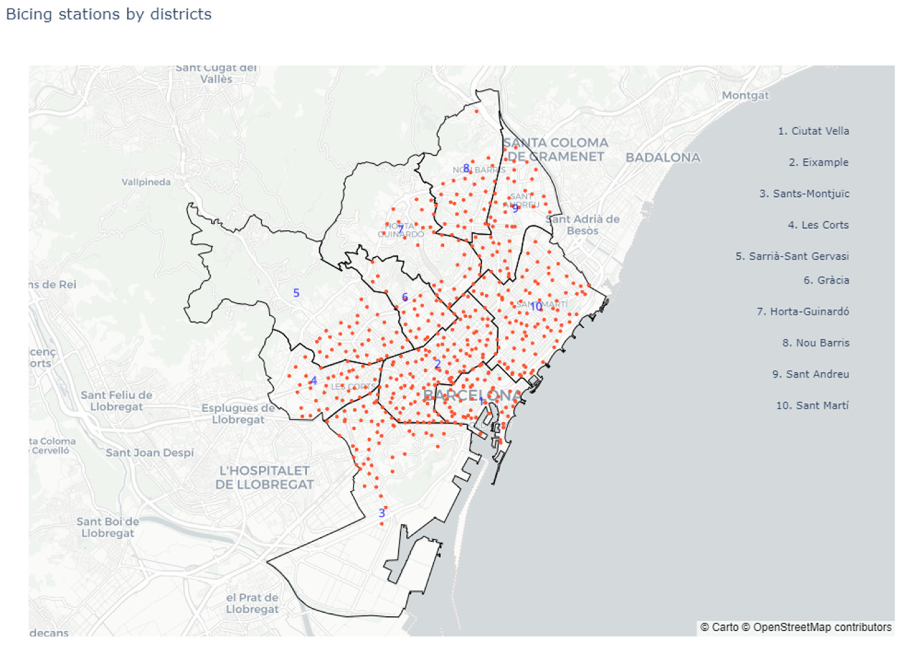
While the data provided by the Barcelona open data portal on the Bicing service are extensive, these are insufficient to fully meet this study’s objectives. For this reason, additional sources were incorporated. The rationale for using these auxiliary datasets is outlined below. For instance,
Figure 1 illustrates the distribution of stations by district. Although the open data portal provides the postal code (CP) for each station, it does not directly indicate its corresponding district. To bridge this gap, the Barcelona GeoPortal [
32], which offers detailed geospatial information about the city, was used. Additionally, while the open data portal provides the population count for each district, it does not break this information down by postal code, and certain postal codes span multiple districts. By leveraging GeoPortal, it was possible to establish relationships between population, station locations, and districts, enabling a more detailed descriptive analysis.
Finally, optimizing the work of service operators and ensuring an equitable bicycle distribution requires a precise understanding of travel times between stations for repositioning vehicles. To this end, the Google Distance Matrix API was used to estimate both the road distance and travel time between all station pairs. As a result, two square matrices of 519 rows and columns were created. It is important to note that this approach does not involve estimating bicycle travel times, which are known to be less reliably predicted by this API due to its car-centric routing logic. Furthermore, to simplify the analysis, it is assumed that no unexpected traffic disruptions or real-time incidents significantly alter travel conditions during operations.
3.2. Vulnerability Indices
Metrics are then established to identify vulnerable areas. The first metric is used to identify discrepancies in terms of accessibility between districts. This metric is calculated by considering the dispersion and number of stations, and the resident population in each district.
where
is the median of the minimum distances from each station in district
to the nearest station in the same district,
is the number of stations in district
and
is the population of district
.
On the one hand, a high value implies that the stations are distributed in a dispersed manner within the district, which could indicate less accessibility for users. This variable represents how accessible the stations within the district are based on their proximity. On the other hand, a greater number of stations, , tends to decrease vulnerability since a higher density of stations facilitates access to the bicycle system. Finally, the district’s population indicates the potential demand for the bike-sharing system. The larger the population, the greater the demand for stations and bicycles in the area; so, a higher value of contributes to a higher vulnerability index, reflecting the need for sufficient infrastructure to meet demand. The influence of these factors on the vulnerability index is determined by the parameters and , which weigh the impact of station dispersion, the number of stations, and population size, respectively. In this study, all three parameters are set to 1, meaning each factor is given equal importance in assessing vulnerability. Despite this fact, an analysis of sensitivity was carried out using different combinations of these parameters.
For the calculation of this metric, the values of each variable, , and were previously normalized. This normalization ensures that the values of the different variables are comparable to each other and that there are no biases derived from the original scales since all the values are located around the same standardized range. Once the vulnerability index was calculated for each district, an additional transformation was applied using the Min–Max scaling method, which adjusts the values obtained to be in a range between 0 and 1. This scale facilitates the interpretation of the results since the values closer to 1 represent the districts with the greatest vulnerability, while the values close to 0 represent the least vulnerable districts within the bike-sharing system.
Finally, a complementary metric is proposed to assess the vulnerability of districts at specific times, based on the availability of bicycles at a given time. Unlike the overall vulnerability index (1), which provides a static view of accessibility in each district, this new index seeks to capture fluctuations in bicycle availability in real time. The goal is to highlight districts that are disproportionately affected by shortages during periods of high demand.
where
represents the total number of hours during which the
station in district
has fewer than 2 bicycles,
is the set of stations in district
and
is the number of stations in district
.
The value indicates the frequency of situations in which users might not find bicycles available or in which the station is close to running out of bicycles. This value can be modified according to the level of risk you want to consider.
A high index value (2) indicates that a district has many hours of bicycle unavailability or is at risk of having it in relation to the number of stations.
The mapping of this metric allows us to observe the situation of each district in an intuitive and visual way. The aim is to use these maps as additional information for the operators in charge of redistributing bicycles. Thus, they have more information about the situation. However, they must follow the paths calculated by the optimization models.
3.3. Clustering
The previous section addresses the first objective of the project: to study the vulnerability of the districts. Clustering represents the beginning of the second objective: to achieve equity in the distribution of bicycles. Given the considerable number of time series involved, clustering techniques were applied to identify and group those series that exhibit similar patterns. This grouping enables a reduction in the number of models required to evaluate the predictive performance of each technique considered. Rather than modeling each time series individually during the evaluation phase, a representative model is developed for each group and method. After assessing the performance of these representative models, the best-performing technique is selected. Subsequently, individual models are created for each time series using the chosen technique, allowing for accurate predictions of bicycle availability at each station. This clustering-based approach reduces the evaluation time while supporting robust model selection.
Clustering consists of grouping elements in such a way that those within the same group are as similar as possible, while elements in different groups are as different as possible. Clustering analysis methods can be categorized into supervised or unsupervised learning. Unsupervised learning examines patterns in input data without any prior knowledge about the expected groups, whereas supervised methods focus on discovering patterns in input data from a well-labeled training set. In this case, the aim is to identify groups without prior knowledge about them. Among all the clustering methods, the
K-means algorithm was adopted, following the work carried out in [
33].
The K-means algorithm groups data into K clusters. Initially, K elements are randomly chosen from the data space to act as the initial centroids of each group. Initially, K elements are randomly selected as centroids. The algorithm calculates the distance between each data point and these centroids, assigning each point to the nearest cluster. New centroids are computed as the mean of the data points in each group, and the process repeats iteratively until cluster assignments stabilize.
As explained in [
34], a key decision in this process is determining the optimal number of clusters
K. To address this, two complementary strategies are employed: the Elbow Method and the silhouette coefficient. The Elbow Method evaluates the within-cluster sum of squares, commonly referred to as inertia, which measures the compactness of clusters. Inertia is defined as follows:
where
is a data point,
is the centroid of cluster
,
is the cluster
,
is the number of clusters and
is the distance used to compute the sum. As the number of clusters increases, inertia decreases, but the marginal gain diminishes. The Elbow Method involves plotting inertia against the number of clusters and identifying the point at which the rate of decrease sharply changes—the so-called “elbow”. In this study, a 10% inertia reduction threshold is applied to guide this selection.
Following [
35], the number of clusters is also evaluated with the silhouette coefficient. This metric is used to assess how well separated the samples are. Specifically, it measures how similar each element is to the elements in its own cluster compared to the elements in other clusters. The expression to calculate the coefficient at a given point is as follows:
where
reflects the average distance between element
and all other elements that are in the same cluster and
reflects the average distance between element
and all elements in the nearest cluster (to which element
does not belong).
After calculating the silhouette coefficient for each sample, the average of all coefficients is used as a measure of the quality of the cluster. A value close to 1 indicates well-separated clusters, a value close to 0 indicates overlap between clusters, and a negative value indicates that some samples are in the wrong cluster. Therefore, groups created with the distance that produces an average silhouette coefficient closer to 1 are used.
For the implementation of this method, the
tslearn library [
36] is used, specifically the
TimeSeriesKMeans method of
tslearn.clustering. It should be noted that this method can calculate groups using three options for comparison: Euclidean distance, Dynamic Time Warping (DTW) algorithm and relaxed DTW algorithm. The key advantage of DTW and soft-DTW over Euclidean distance is that DTW allows for the alignment of sequences with different lengths or temporal shifts by dynamically warping the time axis. This makes it possible to capture similar patterns even if they are out of phase over time. In contrast, Euclidean distance strictly compares corresponding points in time, making it sensitive to misalignments and variations in the timing of patterns. However, in the case studied, there is no time lag; therefore, any of the options can be used. The time lag is eliminated in data preprocessing. For greater representation, the original time series, defined over the entire period, is not used. For each series, the hourly average on each day of the week is calculated. By averaging the values by hour and day, daily variations that are not significant for long-term analysis are eliminated, thus achieving a more representative series of the general patterns and eliminating possible noise. The silhouette coefficient is also employed to evaluate and compare the performance of each variant of the
TimeSeriesKMeans method, guiding the selection of the most suitable algorithm for the clustering task.
3.4. Predictive Techniques
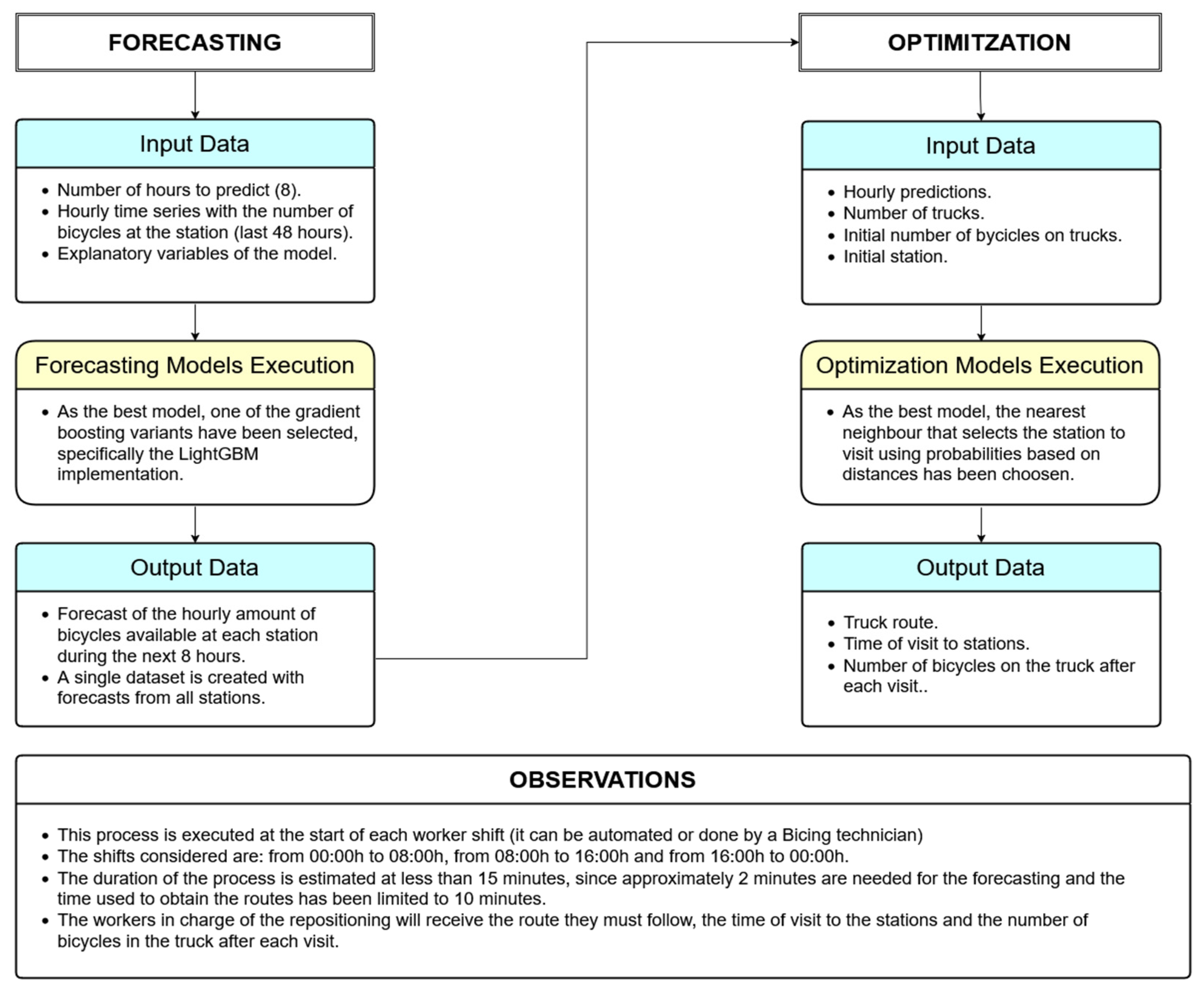
As outlined in the previous section, clustering is used to group stations with similar bicycle availability patterns, helping to reduce the number of models required for evaluating different predictive techniques. These techniques are used to estimate the number of bicycles available at each station. The proposed techniques are models based on gradient boosting and neural networks of the LSTM (Long Short-Term Memory) type. The goal is to generate a prediction for the next 8 h from the time the models are launched. This prediction will serve as input to the optimization models, which will allow the workers in charge of the redistribution of bicycles to know the route they must follow at the beginning of each shift to ensure a good balance in the stations.
Gradient boosting is a machine learning technique widely used today, which has traditionally been used to solve both regression and classification problems. Its popularity is due to its ability to combine multiple weak models (usually decision trees) and produce a robust final model, which achieves good results by iteratively correcting the errors of previous models. Instead of building a complex model from scratch, gradient boosting builds a sequence of simpler models, optimizing performance step by step. The gradient boosting approach is based on a sequential learning process. Unlike other boosting methods, such as AdaBoost, which seek to adjust for classification errors in each iteration, gradient boosting uses the gradient error, calculated at each step, to correct errors from the previous model. Although commonly used in classification and regression tasks, gradient boosting has proven to be useful in the field of time series, especially for prediction problems. Libraries such as
Skforecast [
37] provide several tools that automate data transformation and model validation. In addition,
Skforecast allows for seamless integration of advanced gradient boosting implementations, such as
XGBoost,
LightGBM, and
CatBoost, making it easy to use for prediction tasks. Therefore,
Skforecast is used to create models that use these techniques. To evaluate the predictive performance of each of the aforementioned techniques, the approach of [
38] is followed, which analyzes demand prediction in the cities of Washington D.C. and Konya.
While gradient boosting is effective in capturing complex, nonlinear patterns in data by using multiple simple models, LSTM networks are capable of modeling long-term dependencies. Because of their ability to remember important information over long periods of time and discard irrelevant information, they are especially useful in time series analysis. LSTM networks are an advanced type of recurrent neural networks (RNNs), which differ from traditional RNNs by their internal architecture, which is composed of several gates that regulate the flow of information. The three main ones are the entrance door, the forgetting door, and the exit door, which allow one to decide what information to keep, what information to forget, and what information to use in the current step. This structure allows LSTMs to overcome the gradient fading problem, which plagues conventional RNNs, allowing LSTMs to learn long-term dependencies. As with gradient boosting methods, LSTMs require a large amount of data to be able to generalize correctly, which fits this use case [
39]. In addition, the
Skforecast library also has functionalities that allow the architecture of these neural networks to be determined, facilitating their implementation to obtain accurate predictive models.
In any prediction model, the choice and definition of explanatory variables plays a crucial role in the performance and accuracy of the model. These variables are elements that the model uses to learn patterns and make predictions about the target variable. The selected variables and the reasoning behind their inclusion in the predictive models that were created are described below. The example presented to predict the demand for bicycles by station by Joaquín Amat Rodrigo and Javier Escobar Ortiz in
Skforecast [
37] is followed.
The variables used can be classified into three families: calendar-based, sunlight-based, and holiday-based variables, such as day of the week, sunrise time, and holiday day, respectively. Calendar variables have a repetitive or periodic nature that is not well represented in their raw form. To capture this cyclicality, they are transformed using sine and cosine functions, allowing the model to recognize patterns without imposing an artificial linear order that could distort the results. In many cases, the effect of an explanatory variable on the target variable depends on interactions with other factors. This phenomenon, known as variable interaction, can be captured by generating new features derived from existing ones. These engineered features help the model uncover hidden patterns, enhancing its predictive performance. In this study, such features were created using
scikit-learn’s
PolynomialFeatures class [
40].
Finally, to evaluate the performance of the predictive models and select the most appropriate technique, the Mean Absolute Error (MAE) is used. This indicator measures the average of the absolute differences between the values predicted by the model and the actual values observed:
where
represents the actual values,
corresponds to the predicted values, and
n is the total number of observations.
3.5. Optimization Techniques
After determining the most suitable predictive technique for this use case, predictive models are developed for all stations in the city. As previously mentioned, the outputs of these models serve as inputs for the optimization algorithms, which aim to design worker routes that ensure a balanced distribution of bicycles.
Given the NP-hard nature of the problem, which encompasses well-known combinatorial problems such as the Traveling Salesman Problem (TSP), the Vehicle Routing Problem (VRP), and the Capacitated Pickup and Delivery Problem (CPDP), obtaining exact solutions in real-time is computationally infeasible. Therefore, instead of presenting an exact mathematical formulation, this study focuses on providing a comprehensive explanation of the employed algorithms, complemented by operational diagrams to elucidate their functionality.
Specifically, two constructive algorithms are selected. These algorithms follow a step-by-step approach, progressively building solutions from scratch to completion. At each stage, they assess specific criteria to determine the next station to visit. The factors considered in these decisions are detailed below. However, before that, it is necessary to define the objective function of the problem.
The goal is to minimize the number of instances in which stations are at risk of overcrowding or shortages. A station is classified as at risk of overcrowding if, at any given time, the predicted number of bicycles exceeds three-quarters of its total capacity. Conversely, a station is considered at risk of stock-out if predictions indicate it has 0 or 1 bicycles available.
In [
41], preventing station overcrowding is prioritized, as the inability to return bicycles due to a lack of available docking spaces causes immediate inconvenience and potential delays. The same principle is followed here, applying a higher threshold for detecting overcrowding and a lower threshold for identifying potential stock-out situations. While bicycle shortages also pose challenges, users can typically find nearby alternatives through the service app, making this issue relatively less critical. To address overcrowding, a broader threshold is established to identify stations at risk, enabling proactive intervention before occupancy levels approach maximum capacity.
It is important to note that the goal is not merely to count how many stations are at risk, but to minimize the total number of instances in which all stations experience these conditions. This means that if a station remains at risk for multiple consecutive hours, each of those hours is counted as a separate occurrence, increasing its impact on the objective function. In other words, the focus is not only on the number of affected stations but also on the frequency and duration of risk situations, providing a more accurate measure of their overall impact on the system.
Working with Open Data Barcelona presents certain limitations that must be considered. There are no publicly available data on Bicing’s redistribution operations, including the number of vehicles assigned to bicycle transfers, their load capacities, or the time required for loading and unloading at each station. These data gaps can impact the accuracy of the analysis and optimization models.
To address these limitations, several assumptions have been made. The fleet is assumed to consist of three vehicles, each with a capacity of 50 bicycles, starting their routes at half capacity. The estimated loading or unloading time at each station is set at two minutes. The designated starting point for all redistribution routes is Gran Via de les Corts Catalanes 760 (Station 1), selected for its central location in Barcelona. At the end of their shifts, workers must return the vehicles to this station to ensure a smooth transition for the next team. Additionally, the number of bicycles loaded or unloaded at each station is fixed. If a station is visited, a third of the total docking capacity is either added or removed.
These assumptions establish an initial framework for developing a redistribution solution. However, they remain flexible and can be refined in future studies to better align with real-world conditions. With the objective function and assumptions defined, the construction algorithms used in this study are now described.
The first algorithm is based on the nearest neighbor approach, adapted to prioritize stations at risk of overcrowding or shortages. The second algorithm builds on this method by incorporating probabilistic elements to expand the search space.
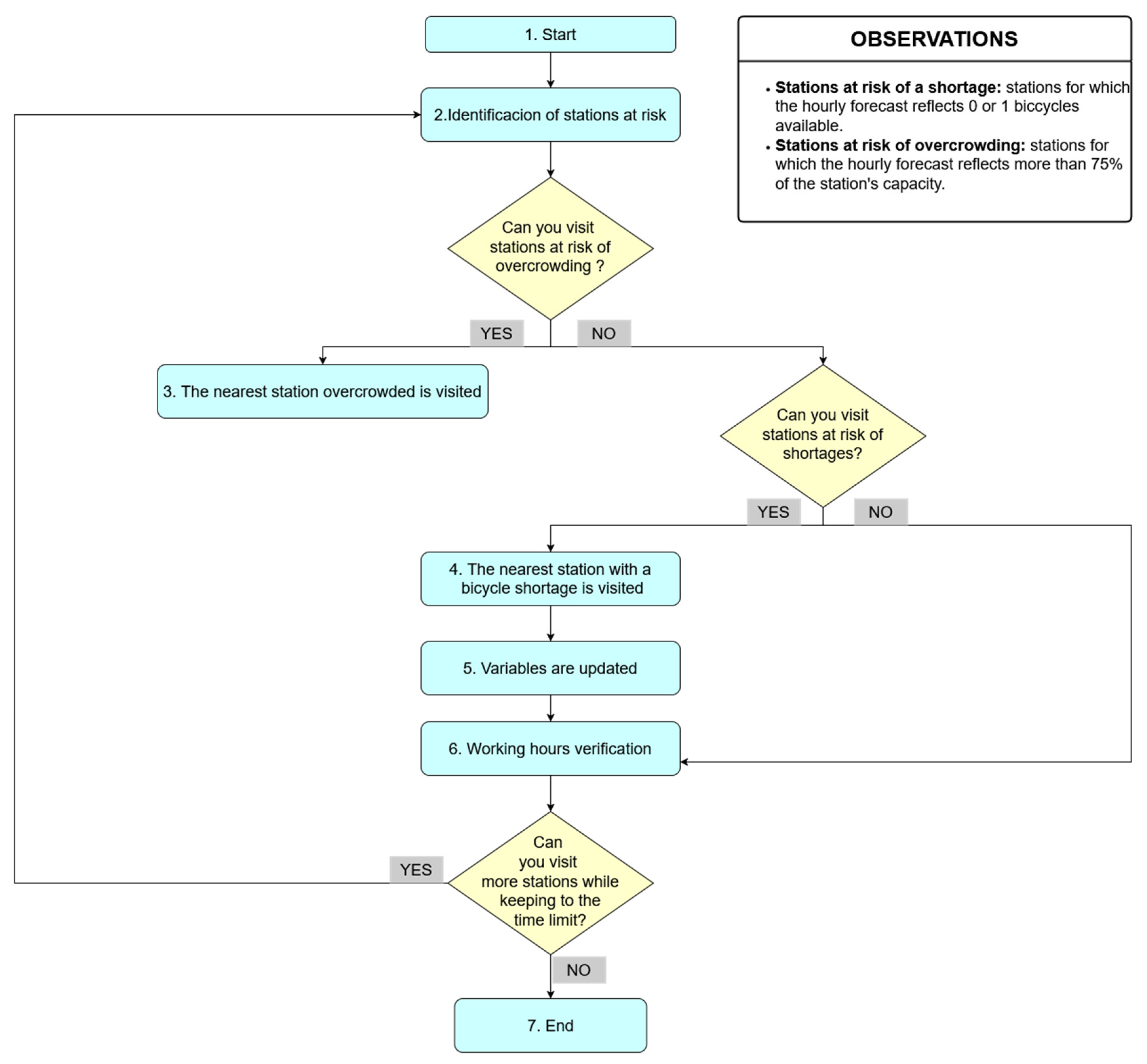
In the field of route optimization, the nearest neighbor algorithm is widely used to construct efficient solutions. In this study, an adapted version is applied to the Bicing system.
Figure 2 outlines the steps followed, integrating the necessary modifications for this specific problem.
The process begins with vehicles departing from the central station. The system first identifies critical stations, distinguishing between those at risk of running out of bicycles and those facing overcrowding. If overcrowded stations are detected, the nearest one that aligns with the truck’s capacity is prioritized for a visit. If the vehicle cannot accommodate the necessary transfer, it proceeds to stations with bicycle shortages, selecting the closest feasible option. After each station visit, key variables are updated, including the truck’s position, the number of bicycles at the station and in the vehicle, and the total time spent on the route. If no station is visited, the truck remains in place, and the remaining time is adjusted based on upcoming needs. This process repeats until the working shift is nearly complete, at which point the vehicle returns to the central station, finalizing the route and recording the sequence of stations visited along with the number of bicycles transported.
This algorithm, adapted for the Bicing system, enables the creation of efficient redistribution routes that prioritize the network’s most urgent needs. Additionally, it continuously accounts for the time required for each task, ensuring that workers complete their shifts without exceeding time constraints. As a result, the algorithm not only improves system balance and user satisfaction but also enhances the efficiency and working conditions of maintenance staff.
However, one significant limitation of this algorithm is its deterministic nature. By constructing a predefined solution based on immediate proximity and fixed constraints, it does not explore alternative routes that could potentially further optimize the number of interventions required.
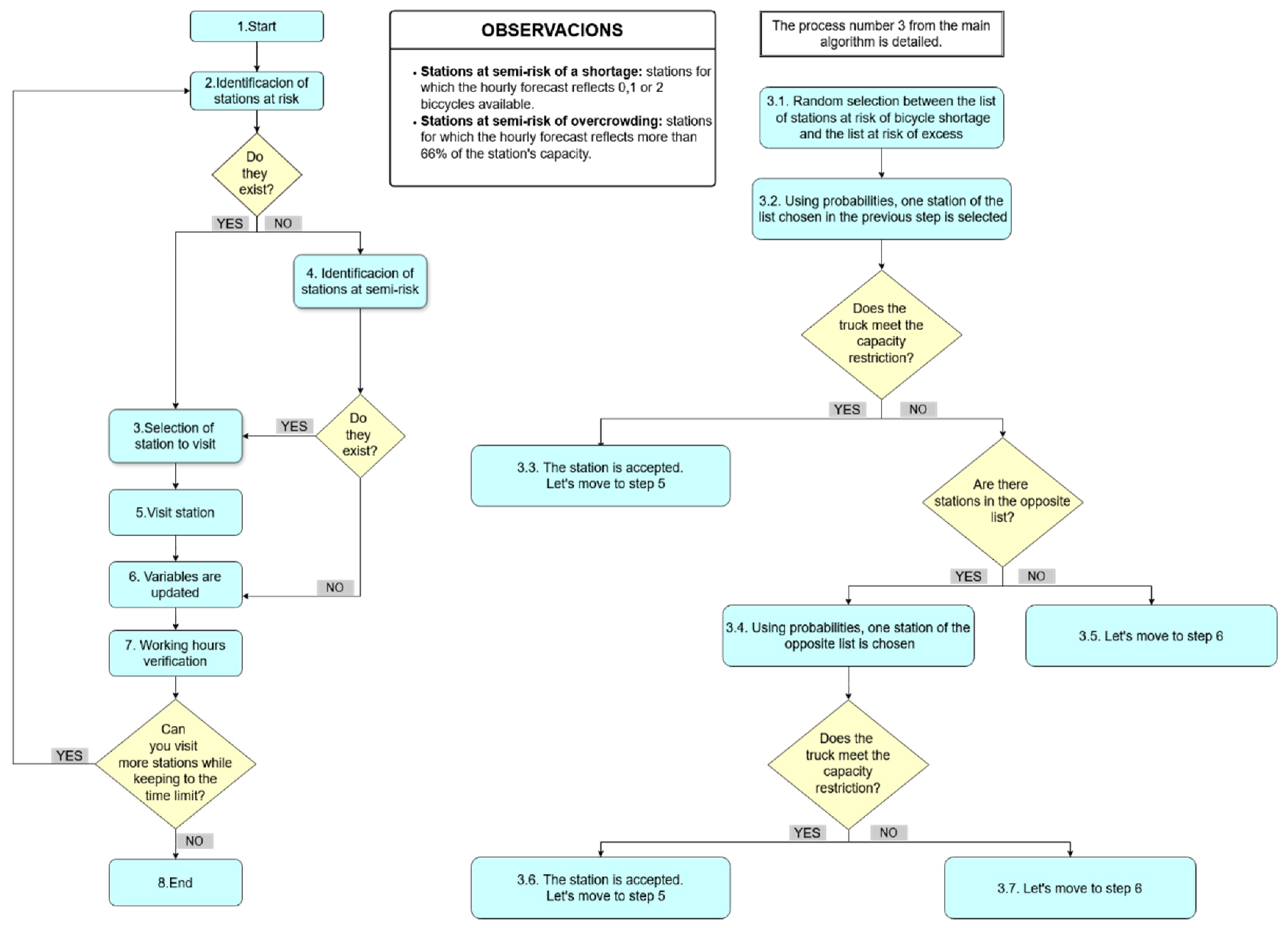
Figure 3 presents the structure of the nearest neighbor algorithm with probabilities, an improved variant of the previous approach. To eliminate the deterministic nature of the nearest neighbor’s algorithm and explore a wider range of solutions, probabilities are introduced in the station selection process. Instead of always selecting the closest station, a probability-based mechanism is implemented to determine which station to visit among those at risk of overcrowding or shortages.
The probabilities are assigned based on proximity, where the closest station receives the highest probability of being selected. The probability decreases progressively as the distance increases. Specifically, the probability for the nearest station is calculated as ; for the second closest station, it is , and so on, where n represents the total number of stations at risk. This method ensures that decisions prioritize nearby stations but also incorporate a probabilistic element that allows for a broader set of potential solutions.
Additionally, the previous rule prioritizing visits to stations at risk of overcrowding over those with shortages is removed. Now, both categories have an equal probability of being chosen as the next destination, making the algorithm more adaptable. This balance can be adjusted according to specific problem requirements.
Another key improvement is the expansion of the range of stations that can be visited. In the previous model, vehicles could only serve stations explicitly identified as at risk in at least one of the hourly predictions. While this approach ensures focused intervention, it may also be overly restrictive, limiting vehicle action when no stations are flagged as critical or when a truck has no bicycles to unload (or space to load more).
To prevent the algorithm from becoming inactive in such cases, a new approach is introduced. The primary focus remains on stations at risk of overcrowding or shortages, provided the truck can effectively assist them. However, if vehicle capacity or visit constraints prevent action at these stations, the algorithm adapts by considering semi-risk stations. A station is categorized as being at semi-risk for overcrowding if, at any predicted hour, the number of bicycles is expected to exceed two-thirds of its total capacity. Similarly, a station is considered as being at semi-risk for shortages if, at any predicted time, it is projected to have only 0, 1, or 2 bicycles available. This added flexibility enhances redistribution efficiency, ensuring that vehicles continue operating even when high-priority stations cannot be served immediately.
The algorithm runs for a predefined time, generating multiple potential solutions. Ultimately, the solution that minimizes the objective function is selected as the optimal redistribution plan.
Alternative neighborhood strategies, shown in
Table 2, are analyzed and compared with the previous methods proposed, but deemed unsuitable for the specific characteristics and objectives of this project.
Although clustering techniques such as k-Means combined with nearest neighbor search can be effective in routing problems, they are not appropriate in this case. The bike-sharing redistribution problem involves a Pick-Up and Delivery structure, where stations have fundamentally different roles (either needing to receive or to provide). There are instances where all the stations within a district may simultaneously experience high occupancy, or conversely, all may face shortages. This uniform behavior across stations renders the strategy of assigning trucks exclusively to predefined areas ineffective. Therefore, a decision was made to avoid using algorithms that first divide the territory into zones before establishing redistribution routes.
Tabu Search and Variable Neighborhood Search (VNS) are advanced metaheuristics well known for their ability to escape local optima and find high-quality solutions. However, their computational cost is considerably higher. Given the real-time demands and the large scale of the Barcelona bike-sharing system, such methods are impractical for direct application. The time required to compute a solution with these approaches would be incompatible with the operational needs of a dynamic, real-world environment.
Finally, although Randomized Search methods could offer high exploration capabilities, their high variability and computational expense make them less appropriate for consistent, time-efficient planning in an operational bike-sharing context.
Thus, the selected methods—Deterministic and Probabilistic Nearest Neighbor—represent a practical compromise between exploration, quality of solutions, and computational efficiency, meeting the specific requirements of this real-world application.
4. Analysis Results
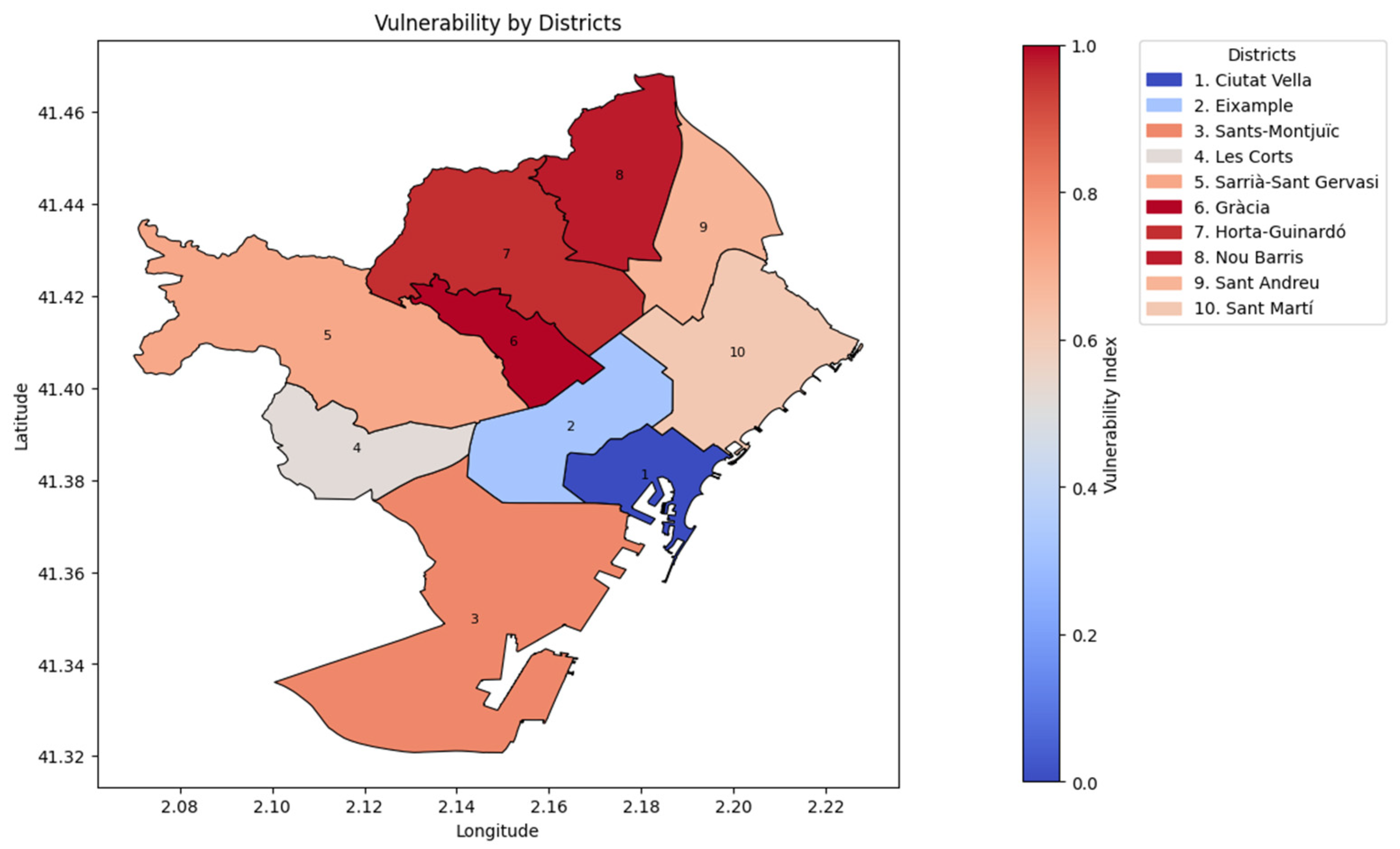
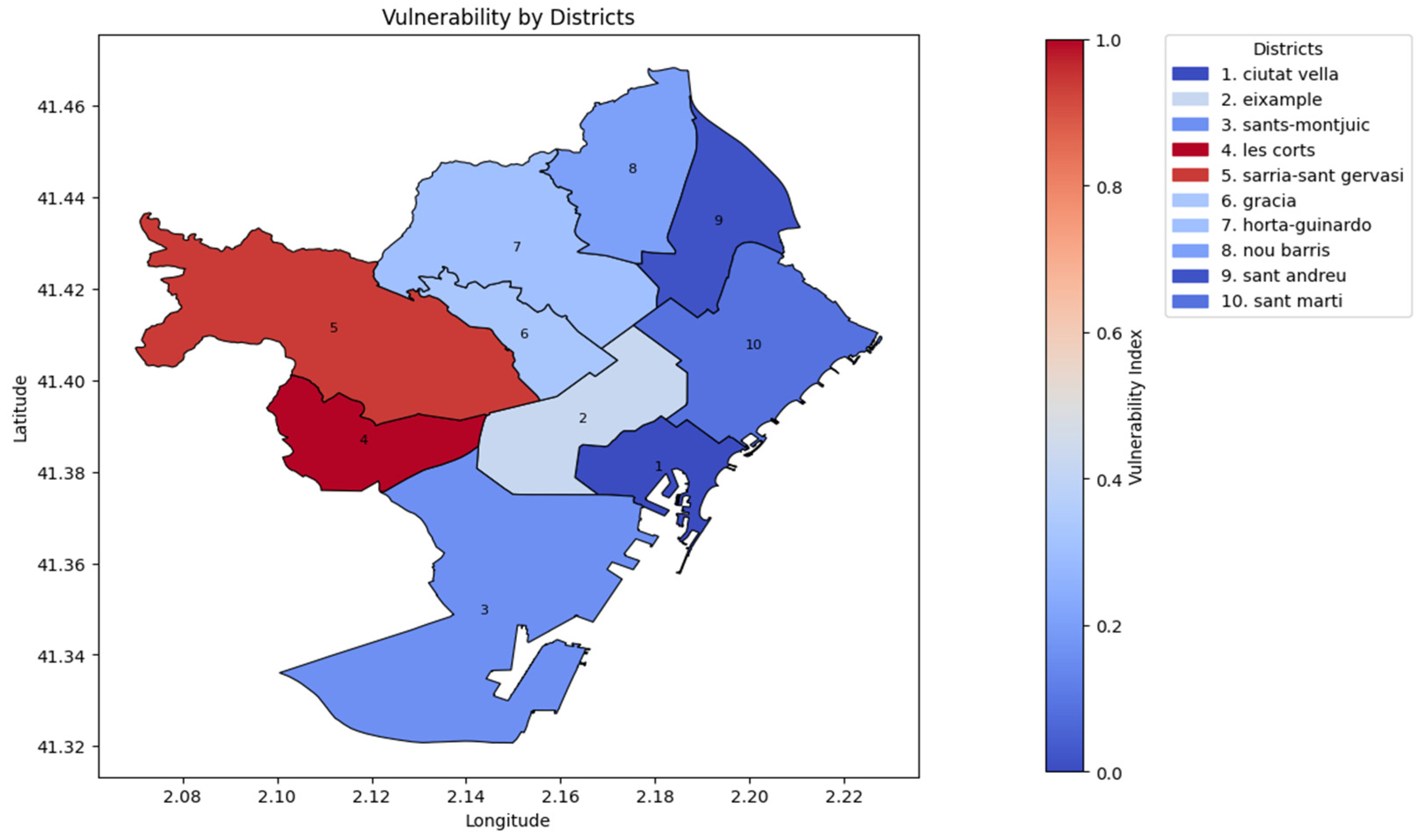
Table 3 and
Figure 4 display the vulnerability index calculated for each district, obtained from Equation (1). This composite index integrates three key variables—station density, station dispersion, and resident population—with each factor assigned equal weight to ensure a balanced assessment of accessibility. The resulting values highlight disparities in service accessibility across neighborhoods, identifying districts where the current bike-sharing infrastructure may be insufficient relative to local demand.
The most vulnerable districts—Gràcia, Nou Barris, and Horta-Guinardó—are characterized by low station density and high station dispersion, which significantly reduce accessibility for users. Conversely, Ciutat Vella and Eixample show low vulnerability levels owing to a higher density of stations, shorter inter-station distances, and greater investment motivated by their historical and economic importance.
In general, outer districts tend to exhibit higher vulnerability, except for Les Corts. As shown below in the clustering analysis study, this result is consistent with the expected dynamics of urban mobility, where flows often originate in peripheral areas and concentrate towards the central districts, increasing the demand in the center and justifying greater infrastructure investment there. Therefore, it can be considered that, at a general level, the existing infrastructure is appropriately organized to support the main mobility patterns of the city. However, specific cases of underserved areas may still exist and should be periodically analyzed to ensure equitable access across all neighborhoods.
To validate the robustness of the vulnerability index and to understand how sensitive the results are to the weight assigned to each factor (distance, number of stations, and population), a sensitivity analysis was performed. This analysis systematically varies the parameters α (distance), β (stations), and γ (population) used in the index formula.
Table 4 summarizes the outcomes under different weighting scenarios. When distance is given more weight (α = 1) and the number of stations and population are given less (β = γ = 0.5 or 0.25), Gràcia consistently appears as the most vulnerable district, and Ciutat Vella as the least vulnerable. When station density is prioritized (β = 1) over distance and population (α = γ = 0.5 or 0.25), Gràcia again emerges as the most vulnerable, while Eixample becomes the least vulnerable. When population is emphasized (γ = 1), new patterns appear: Sant Martí and Nou Barris become the most vulnerable districts depending on the weights of distance and stations, indicating that population-related demand pressure plays a more significant role in these areas. In contrast, Ciutat Vella is again the less vulnerable district.
This sensitivity analysis confirms that the identification of Gràcia as the most vulnerable district is robust across various weighting schemes. It also reveals that population can be a critical factor in specific districts like Sant Martí and Nou Barris, suggesting that different investment strategies might be needed depending on the local context and policy priorities to improve the infrastructure of the system.
In conclusion, the vulnerability analysis, combined with the sensitivity study, provides a robust and nuanced understanding of structural weaknesses within the bike-sharing system. These insights are valuable for guiding infrastructure investment and ensuring equitable access across districts. However, to further enhance system management and respond effectively to fluctuating user demand, it is equally important to understand the temporal and behavioral dynamics of station usage. In this context, clustering analysis complements the vulnerability framework by revealing patterns in station-level activity, enabling a more adaptive and demand-responsive strategy.
Clustering analysis was employed to identify groups of stations with similar usage patterns over time. Rather than using the full hourly dataset from 2022 to 2023, which would be computationally intensive, a weekly hourly average was computed. This involved calculating the mean number of available bicycles for each hour of each weekday in each station across the entire analysis period. The resulting time series preserved the essential temporal characteristics of usage while simplifying the dataset, thus improving interpretability and computational efficiency.
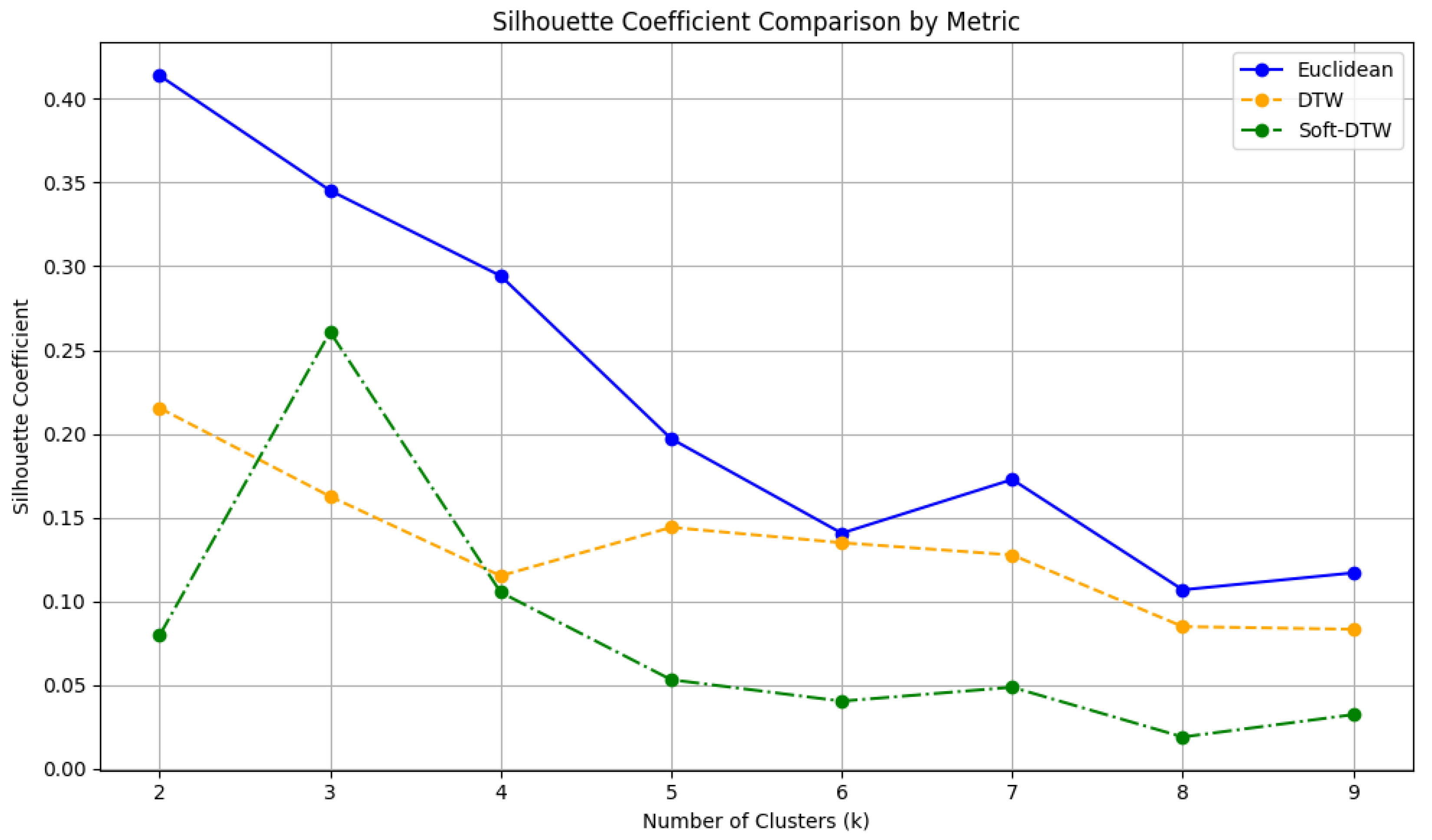
The first methodological decision in the clustering analysis involves determining the optimal number of clusters and selecting the most appropriate distance metric for time series comparison. As discussed earlier, we employed the TimeSeriesKMeans algorithm, which supports various distance measures. To guide these decisions, we relied on two widely used techniques: the Elbow Method and the Silhouette Coefficient.
Initially, we computed the Silhouette Coefficient for values of
K = 2 to
K = 9, using three different distance metrics: Euclidean distance, Dynamic Time Warping (DTW), and Soft-DTW. Across all tested values of
K, the Euclidean distance consistently yielded the highest silhouette scores, indicating more cohesive and well-separated clusters. Based on these results, Euclidean distance was selected as the preferred metric, as illustrated in
Figure 5.
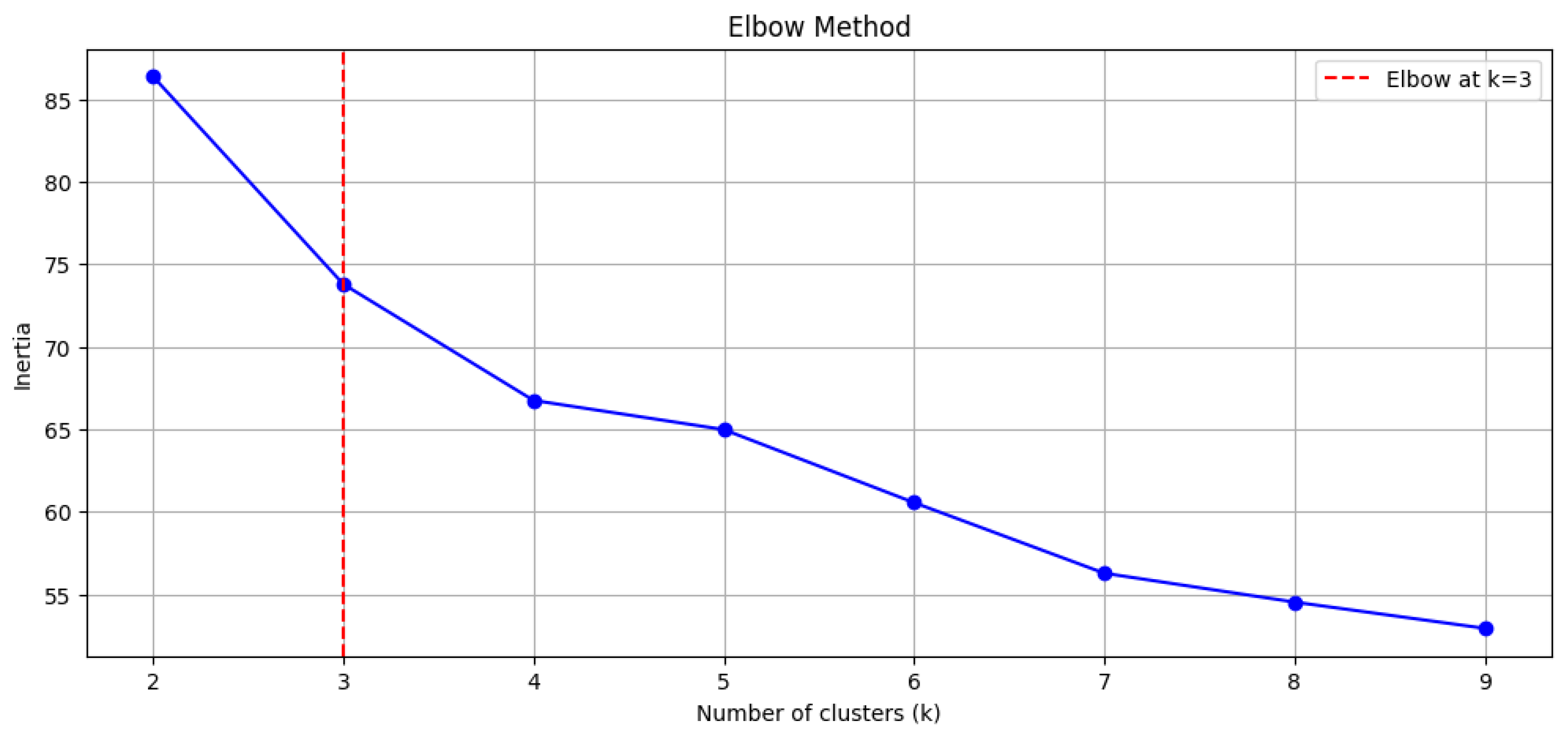
Subsequently, the Elbow Method was applied to determine the optimal number of clusters by plotting the inertia (within-cluster sum of squares) for
K = 2 to
K = 9. In this study, a 10% inertia reduction threshold was used to identify the point beyond which adding additional clusters yields diminishing returns. The analysis revealed an inflection point at
K = 3, as shown in
Figure 6, indicating that three clusters strike a suitable balance between explanatory power and model simplicity. Although the Silhouette Coefficient peaked at
K = 2, we chose
K = 3 to capture greater variability in usage patterns across stations, which aligns with the exploration goals of the analysis.
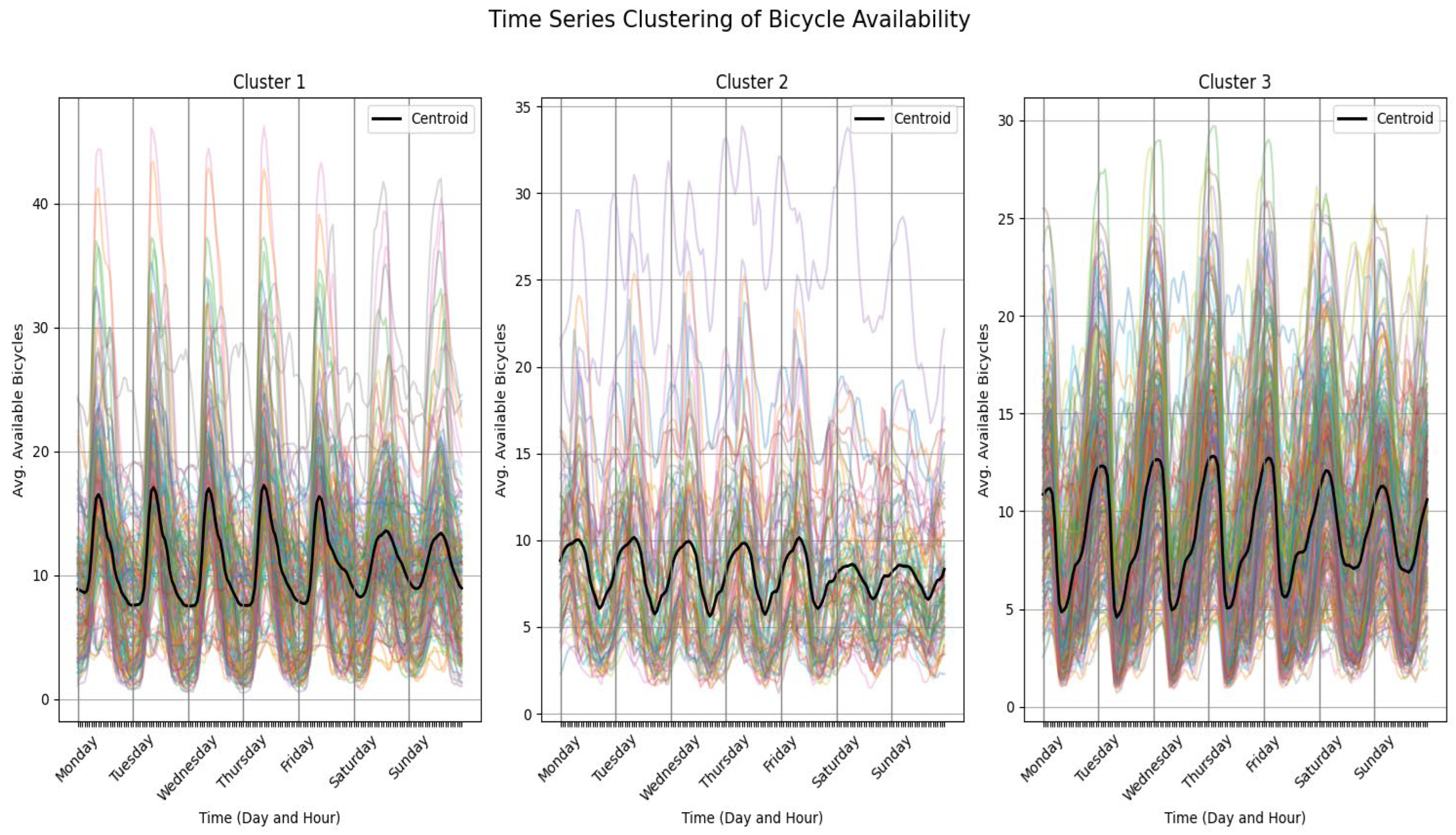
After observing that Euclidean distance yields the best results, the clustering analysis was carried out using this distance measure with
K = 3 clusters, as determined through the Elbow Method and the 10% inertia reduction threshold.
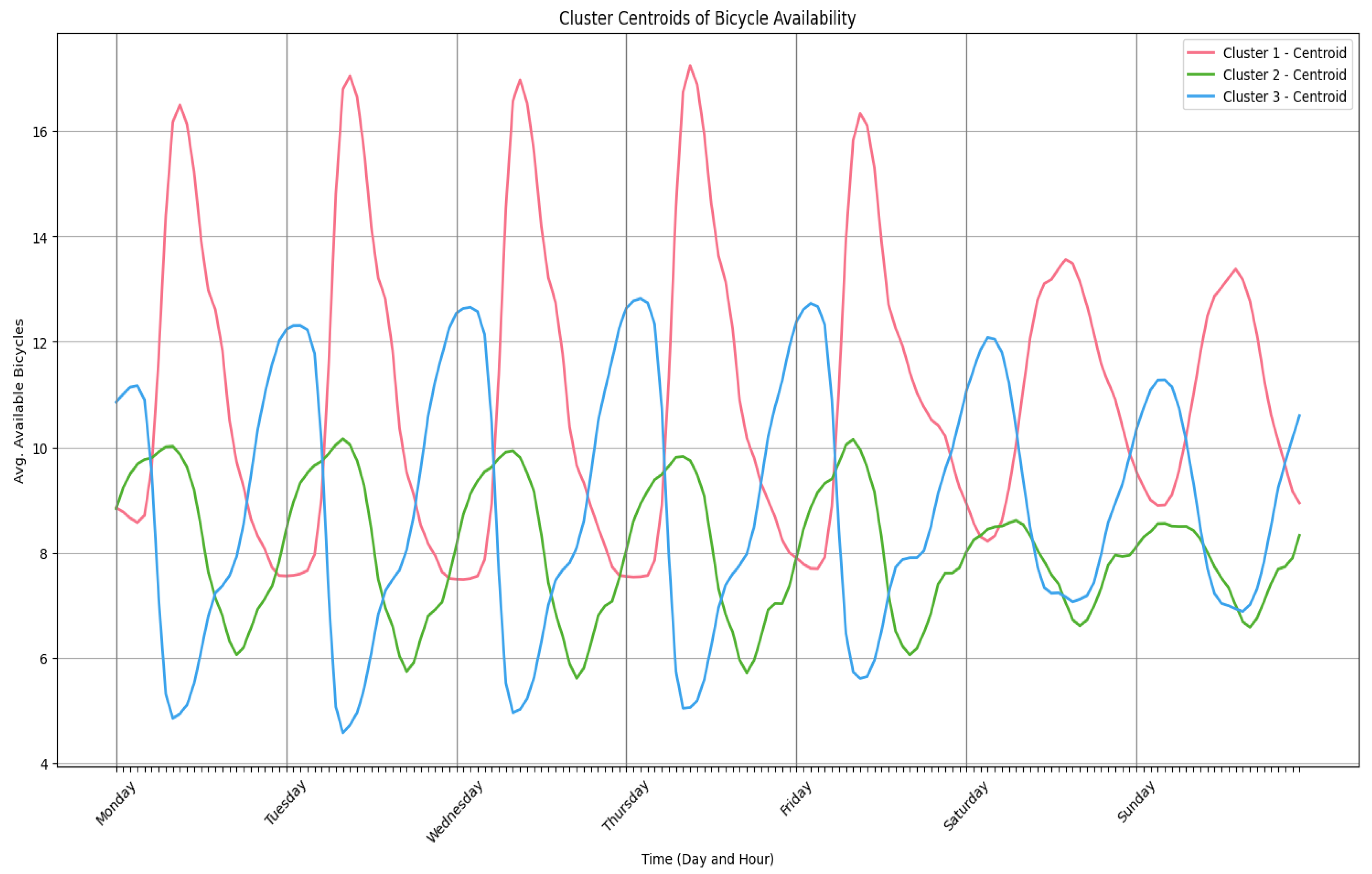
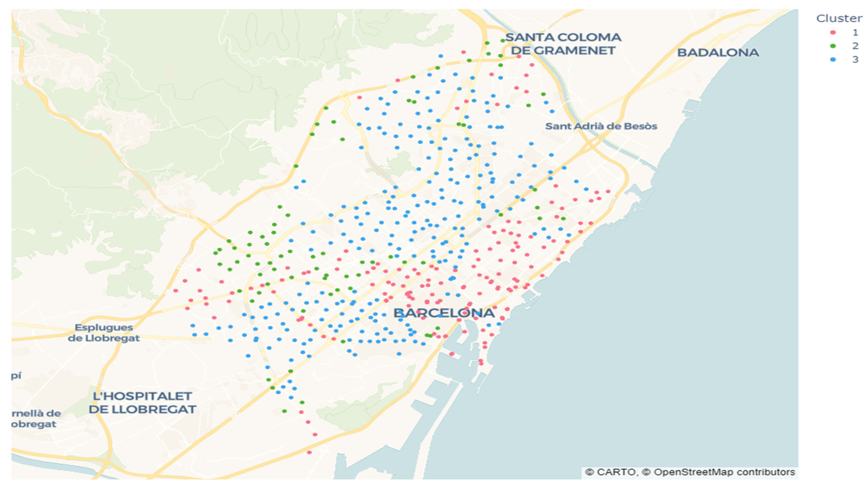
Figure 7 illustrates the weekly patterns of bicycle availability, while
Figure 8 shows the centroids of each cluster.
The first and third clusters exhibit opposite behaviors in terms of bicycle availability: when stations in cluster 3 are overcrowded, those in cluster 1 are empty, and vice versa. In contrast, cluster 2 stations display more stable usage patterns with fewer fluctuations, indicating balanced demand.
Figure 9 links these results to geographic distribution; l’Eixample, Sant Martí, and Ciutat Vella act as bicycle receivers in the early morning due to their concentration of offices, shops, and universities. Many users travel from residential areas to these districts, causing morning station saturation and leaving few bicycles available. Later, as work hours end, stations in these areas become depleted. A similar pattern is observed near the Diagonal, a major thoroughfare connecting high-density office and university zones.
In contrast, districts such as Gràcia, Horta-Guinardó, Les Corts, and Sants-Montjuïc show the opposite trend. Morning departures create shortages around noon, followed by station saturation in the late afternoon. Sarrià-Sant Gervasi exhibits a different pattern with less pronounced seasonality, likely due to lower Bicing usage. The district’s hilly topography may make cycling less attractive, reducing service demand compared to flatter areas.
Sant Andreu and Horta-Guinardó display a mix of all clusters, suggesting varied usage patterns. A station-specific analysis is needed to fully understand this diversity.
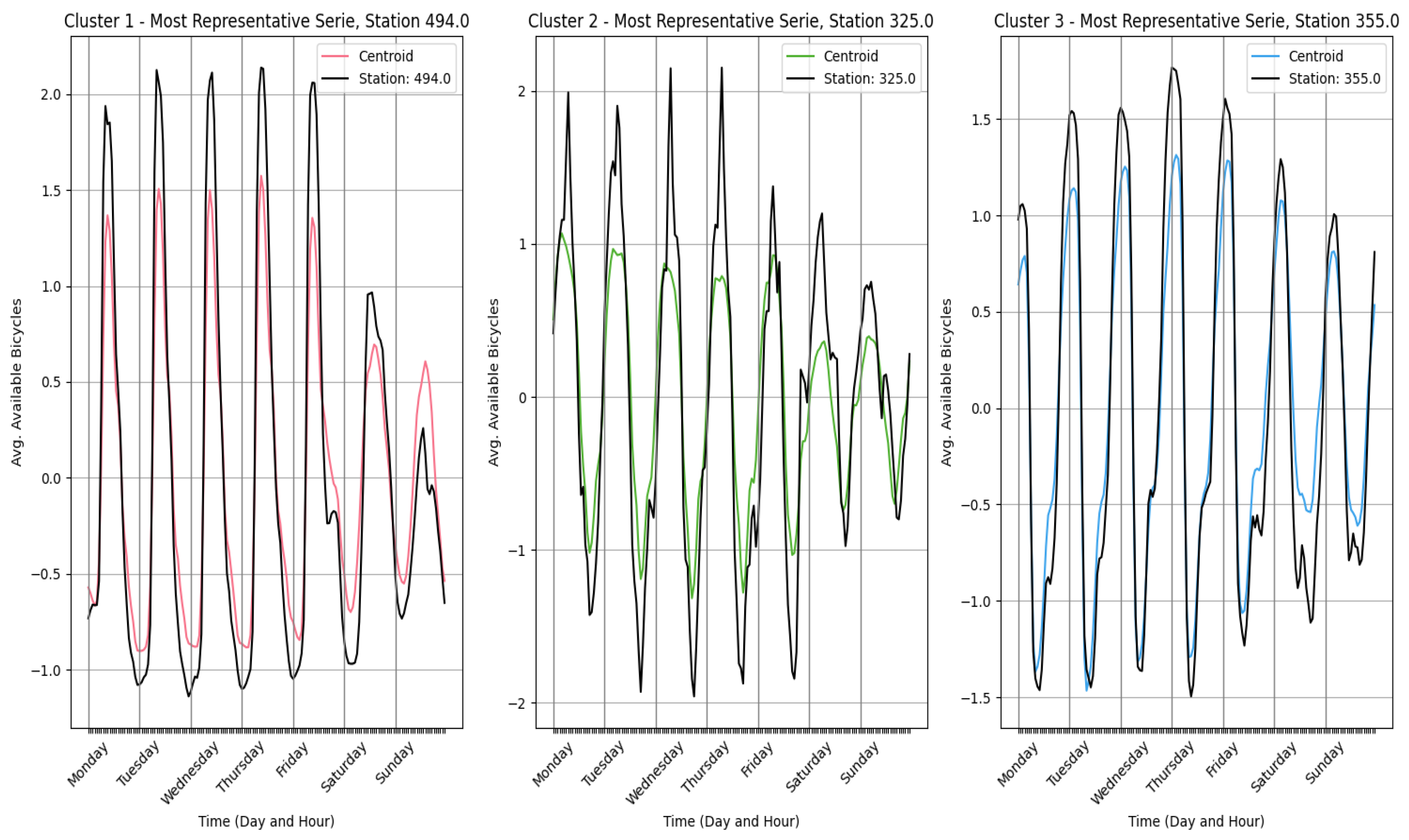
To conclude the clustering analysis,
Figure 10 presents the most representative time series for each cluster. These representative series best match the average behavior of their respective groups. In time-series clustering, centroids represent the average pattern, while representative series are the individual time series that most closely reflect this pattern. Selecting representative series allows for an initial evaluation of predictive techniques using just three time series, significantly reducing computational effort. While individual models are later developed for each station, this step optimizes the predictive modeling process by improving efficiency.
After selecting the three representative series—stations 494, 325, and 355 from clusters 1, 2, and 3, respectively—machine learning models were developed to predict bicycle availability at these stations. Gradient boosting models (XGBoost, CatBoost, and LightGBM) and LSTM networks were chosen due to their ability to capture complex, nonlinear patterns given the large dataset.
The performance of these techniques was evaluated using the available data from 2022 to 2023. To facilitate this evaluation, the dataset was divided into three subsets: the training data, covering the period from 1 January 2022 to 30 April 2023; the validation data, spanning from 1 May 2023 to 30 September 2023; and the test data, which includes records from 1 October 2023 to 31 December 2023.
As mentioned before, the Mean Absolute Error (MAE) was used to validate the choice of the predictive technique.
Table 5 presents the MAE obtained in the test set for each of the implemented models, highlighting the one with the best performance. This compares the accuracy of the models and determines which one is closest to the actual values in the predictions. A lower MAE value indicates that the model more accurately captures patterns in the data.
It is observed that models based on gradient boosting achieve a lower MAE compared to LSTM models. Among gradient boosting options, the results are very similar. In fact, each of the three implementations (LightGBM, XGBoost, and CatBoost) showed a slightly higher performance in one of the clusters. Therefore, the neural networks are discarded and the models based on gradient boosting are selected.
Before continuing, it should be noted that one of the hyperparameters optimized in gradient boosting models is the number of lags used for prediction. In two of the three cases studied, the best result was obtained with 48 lags, i.e., considering as input two days of prior information to predict the next 8 h. In the third case, a single day of previous information was enough. The options evaluated included 24, 48, 72 lags and a combination of point values (1, 2, 3, 23, 24, 25, 167, 168, 169). Although this hyperparameter could be adjusted for each series and achieve an improvement in accuracy, the differences observed are minimal. Therefore, to simplify and reduce the time it takes to create the models, it was chosen to set this value at 48 lags. In this way, gradient boosting models with 48 lags were used for prediction, specifically using the implementation of LightGBM. As with lags, the performance differences observed between the different implementations, XGBoost, LightGBM and CatBoost, were minimal; so, one of these variants was selected for the final models, although any of the others would have been equally valid.
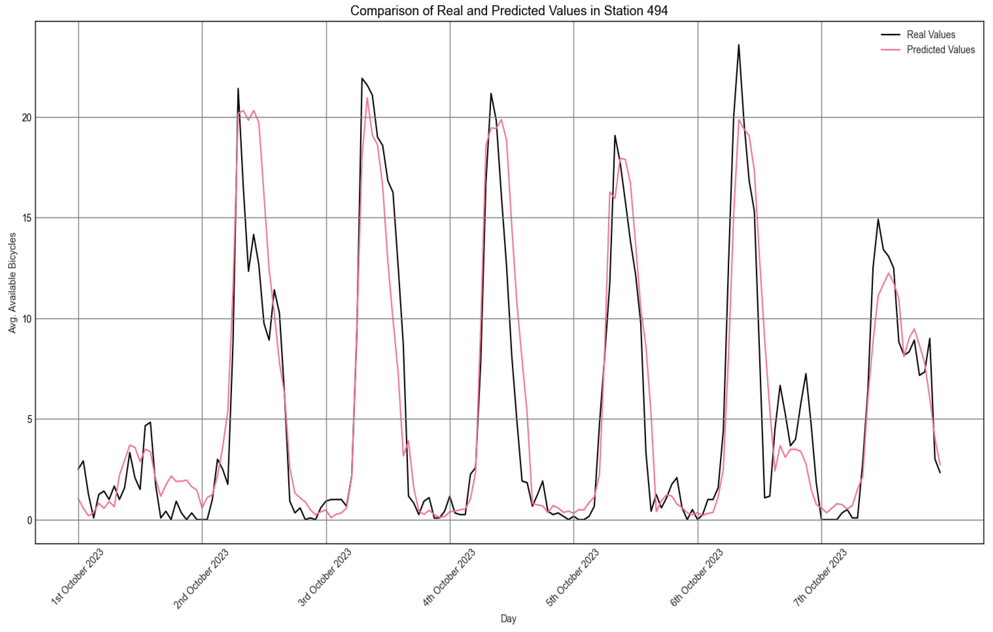
As an example,
Figure 11 shows the prediction for the first week of the test set of the representative station of the first group. Although the time horizon of each prediction is 8 h, it was possible to obtain results for the whole week by applying a validation method called backtesting. This method consists of dividing the test set into multiple successive intervals (in this case every 8 h), making sequential predictions for each of them and updating the model as time progresses. In this way, the behavior of the model can be evaluated over longer periods. This same method was used to compute the MAE values in the above table.
Although the model does not capture all the point variability, it does manage to reflect the seasonal cycle of the series, which is sufficient to anticipate peaks in shortages and saturation.
To conclude the predictive study, the temporal vulnerability index (2) is retrieved.
Figure 12 shows, as an example, the predicted vulnerability for the first day of the test set (during its first 8 h). This graph suggests the need to move bicycles to the districts of Les Corts and Sarrià-Sant Gervasi to avoid the shortage of bicycles suffered by the stations in these districts at that time. It should be clarified that this vulnerability analysis should not be interpreted as an operational roadmap for workers, but as a tool for validating the prediction and as visual support to better understand the situation. The route design to achieve a more balanced distribution of bicycles is made using optimization models, which offer greater reliability in operational decision-making.
Finally,
Table 6 shows the predictive performance of all the time series, organized by cluster. Specifically, the MAE measures how far the model deviates, on average, from the actual number of bicycles available in each prediction. In practical terms, the MAE represents how many there are bicycles on average, and the prediction of the real value differs. In this case, the average error is approximately three bicycles, which indicates a reasonable accuracy in the estimates and allows for validation of the predictive models created.
Once the best predictive technique has been selected and its accuracy has been validated, it is time to integrate these predictions into the optimization models, as they are their input.
Below, the two previously defined optimization models are compared: deterministic nearest neighbors and nearest neighbors with probability. The objective is to analyze, in practical cases, the results obtained with each model to determine which is more appropriate according to the needs of the system.
For this analysis, predictions for 1 October 2023 are used. The predictions are divided into three-time shifts: 00:00 to 08:00, 08:00 to 16:00, and 16:00 to 00:00.
As explained before, the objective function is to minimize the number of times stations are at risk of running out of bicycles (undersupplied) or reaching full capacity (overcrowded).
Table 7 presents the predicted values of this objective function without any modifications, along with the number of stations that experience under-supply or congestion at any given moment.
The first of the comments here is related to the algorithm that includes probabilities. Despite giving greater weight to the nearest stations, the choice of the station to visit according to the probability granted can cause the visit of stations not to be so close. It was therefore decided to reduce the number of stations that can be visited. Instead of considering the n stations that are at risk in each iteration, only a small number of them are considered. Specifically, the tests have been carried out considering the two and five nearest stations.
The algorithms were designed by incorporating the number of vehicles as a parameter, which allows for an evaluation of the impact of increasing or reducing the number of trucks assigned to repositioning tasks.
Table 8 shows the number of stations at risk after the repositioning tasks, depending on the number of vehicles and the algorithm used, highlighting the best algorithm in each situation.
Although the sample used for analysis is not fully representative and does not allow for absolute certainty in decision-making, it provides valuable insights into the performance of the algorithms.
In all cases, the implemented algorithms successfully reduce the original value of the target function. As expected, increasing the fleet size improves the results. Additionally, incorporating probabilities for station selection and generating diverse routes leads to better performance compared to that of a fully deterministic algorithm. However, it is also observed that selecting among multiple stations based on probabilities generally worsens the results, except in specific cases. Therefore, the best approach is to use the algorithm that introduces probabilities (selecting between two stations) and maximizing the number of available vehicles.
Regarding computing times, the deterministic nearest neighbor algorithm generates a route in under one minute, regardless of the number of vehicles used. In contrast, the probabilistic algorithm controls the number of iterations through a time constraint. Specifically, the route construction process is limited to a maximum of 10 min, after which the best solution found up to that point is selected. This time restriction ensures that the optimization process aligns with real operational conditions.
It was estimated that the transition time between worker shifts (the period when one team’s shift ends and another’s begins) is approximately 15 min. During this interval, both the predictive models (trained using gradient boosting) and the optimization algorithms must be executed. The prediction process, which estimates the number of available bicycles at each station, takes less than 2 min. Therefore, the execution of the optimization models was limited to 10 min to fit within this operational window.
As an example,
Table A3,
Table A4 and
Table A5 present the results obtained using the probabilistic algorithm with three vehicles when selecting between two stations. This information will be provided to workers so they can follow the designed routes and stay informed about station conditions.
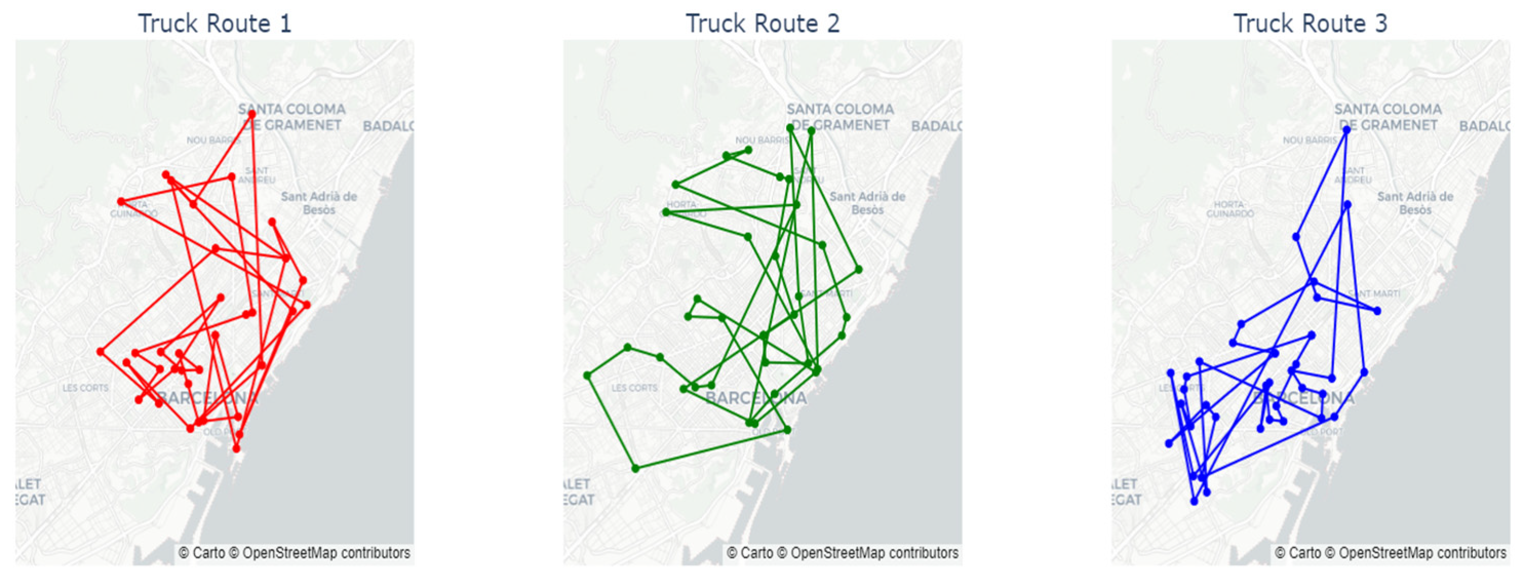
Finally, for this same case, the maps in
Figure 13 show the routes of each of the vehicles. These maps were designed with the aim of interpreting the results obtained. As expected, none of the vehicles remain static in any of the city’s districts, but they move according to the needs of the system.
Previously, it was observed that stations within the same district tend to show similar patterns of behavior. For example, it may happen that all the stations in a district have a high occupancy simultaneously or, on the contrary, that they are all undersupplied. This homogeneous dynamic between stations makes the strategy of assigning trucks exclusively to specific areas ineffective. For this reason, as previously mentioned, it was decided not to use algorithms that first segment by zones and then build the routes. Finally, it should be noted that, in general, the trucks move to nearby stations. However, on specific occasions, they make longer-distance journeys, responding to the priority of visiting stations at risk of shortages or risk of saturation.
It is concluded that the models developed, based on the nearest neighbor algorithm, improve both user and employee satisfaction by streamlining workers’ operations and ensuring a more balanced distribution. Additionally, these models contribute to enhancing urban sustainable mobility and promoting a smarter approach to bicycle repositioning, leading to a more efficient and environmentally friendly transportation system.
6. Conclusions
This study tackles the challenge of bicycle and station imbalance in Barcelona’s Bicing system by optimizing their distribution to enhance accessibility.
The methodology applied consists of three key components. First, a descriptive analysis was conducted. Metrics such as the vulnerability index, distribution maps, and clustering techniques were used. Next, predictive models based on gradient boosting and LSTM neural networks estimated bicycle availability. Finally, optimization algorithms, including the nearest neighbor method and its variants, were designed to minimize station saturation and shortages by proposing efficient redistribution routes.
The results highlight several key findings regarding service accessibility and infrastructure. In general, outer districts are more vulnerable, apart from Les Corts. In contrast, l’Eixample and Ciutat Vella stand out for their high station density. This distribution of resources is logical, as these districts are the central hubs of the city, where most activity is concentrated.
The clustering analysis reveals distinct usage patterns. L’Eixample, Sant Martí, and Ciutat Vella act as bicycle receivers in the early hours of the day. In contrast, Gràcia, Horta-Guinardó, Les Corts, and Sants-Montjuïc show the opposite trend, with a high departure of bicycles in the morning and a return flow later in the day. Other districts exhibit less pronounced and more balanced patterns.
Gradient boosting models effectively predict saturation and shortages, particularly in stations with strong seasonal trends. Additionally, optimization algorithms significantly reduced station imbalances. The nearest neighbor approach, incorporating probability-based decision-making with three redistribution vehicles, led to a 50% reduction in tested scenarios. These optimized routes specify when and how many bicycles should be repositioned, streamlining redistribution efforts.
By integrating predictive and optimization techniques, a robust solution that strengthens system performance has been developed. Additionally, the descriptive analysis provides valuable insights to ensure the proposed solutions address real operational needs. This multi-perspective approach underscores the importance of data-driven strategies in achieving impactful and sustainable results.
Overall, optimizing station and bicycle distribution enhances service efficiency and user satisfaction, and contributes to sustainable urban mobility by promoting a more balanced and resource-efficient transportation system.
Next, we aim to validate our models in collaboration with the Bicing operational team to assess their real-world effectiveness. Following this validation, controlled pilot tests will be conducted to refine the models further and identify any practical limitations. Addressing these challenges in future iterations will enhance the proposed solutions’ overall effectiveness and scalability.


