
Empowering Sustainability: A Consumer-Centric Analysis Based on Advanced Electricity Consumption Predictions


Abstract
1. Introduction
1.1. Background
1.2. Related Literature
1.3. Objectives and Research Questions
1.4. Practical Implications and Study Outline
2. Materials and Methods
2.1. ARIMA and SARIMA Models
- The first step is to check whether the series is stationary. If a time series has a trend average that varies over time or seasonality that varies over specific time periods, then it should be converted to a stationary time series.
- The differencing mechanism is applied. If the time series is not stationary, differencing is applied to make the time series stationary. Take the first difference and check stationarity until it becomes stationary. Seasonal differences should also be controlled.
- Validation samples are created.
- AR and MA are included based on AC and PAC.
- The model becomes ready for prediction.
- Validate the model by comparing the predicted values.
2.2. ETS Model
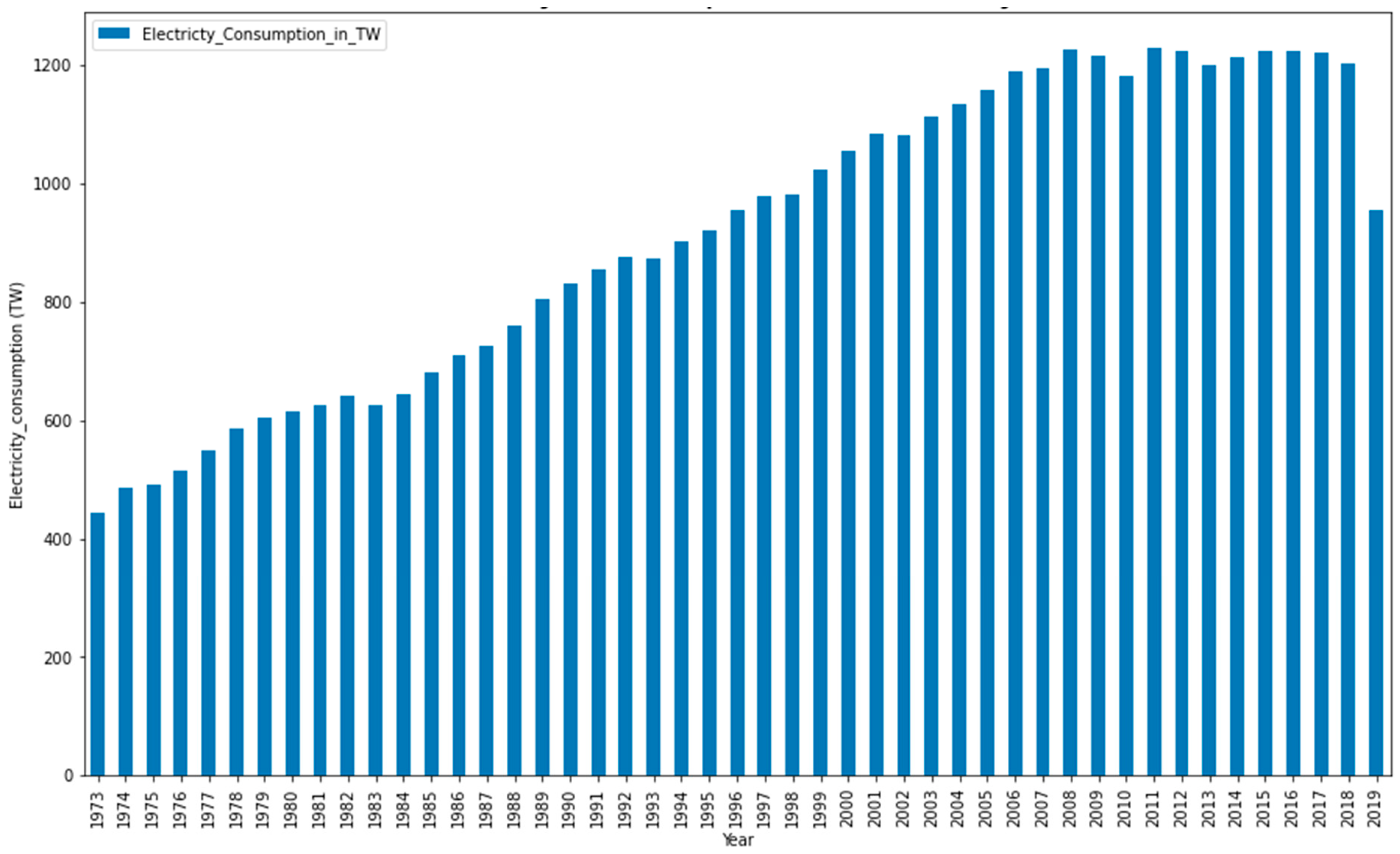
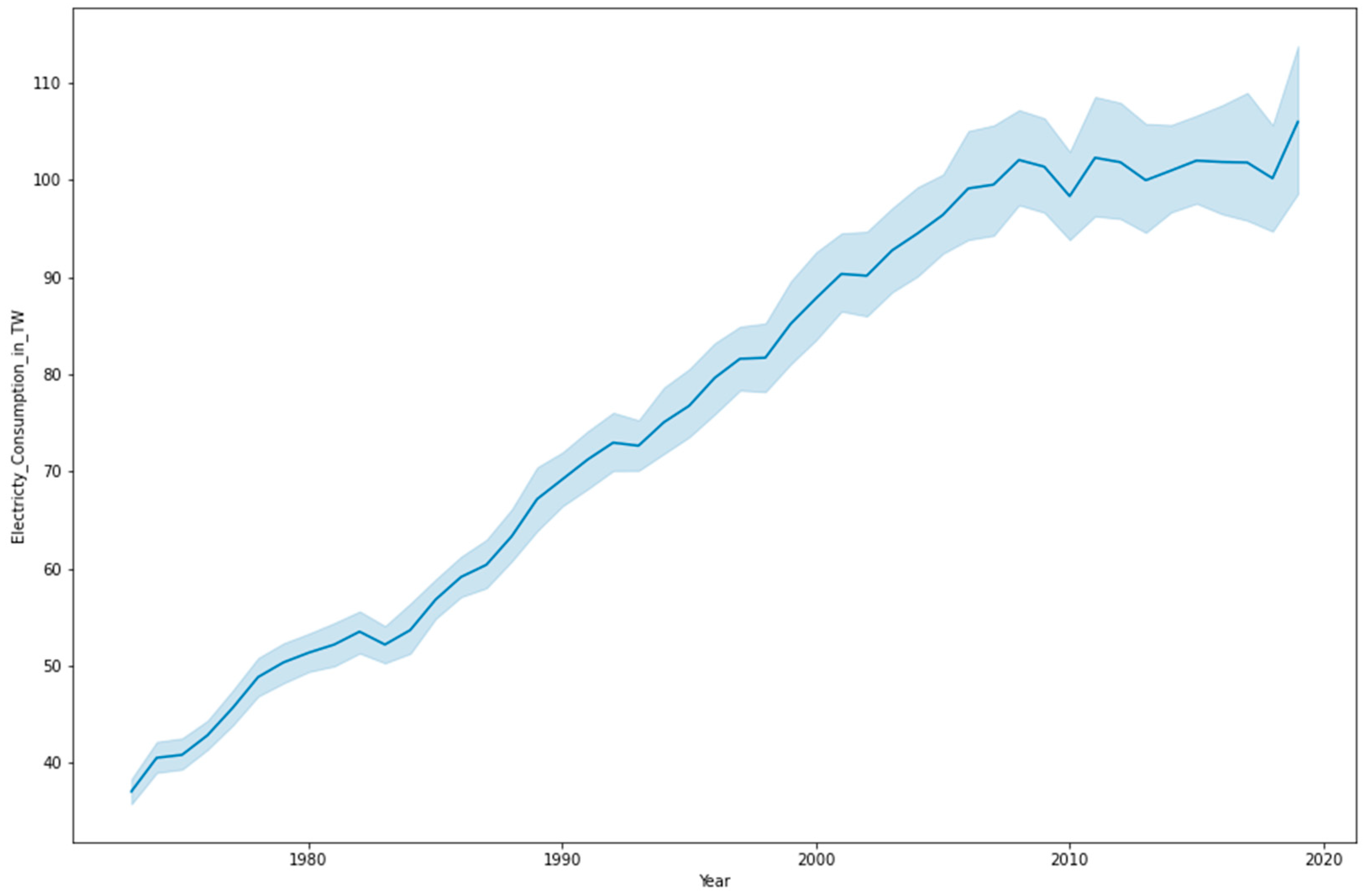
2.3. Dataset
3. Results
3.1. Exponential Smoothing Model Results
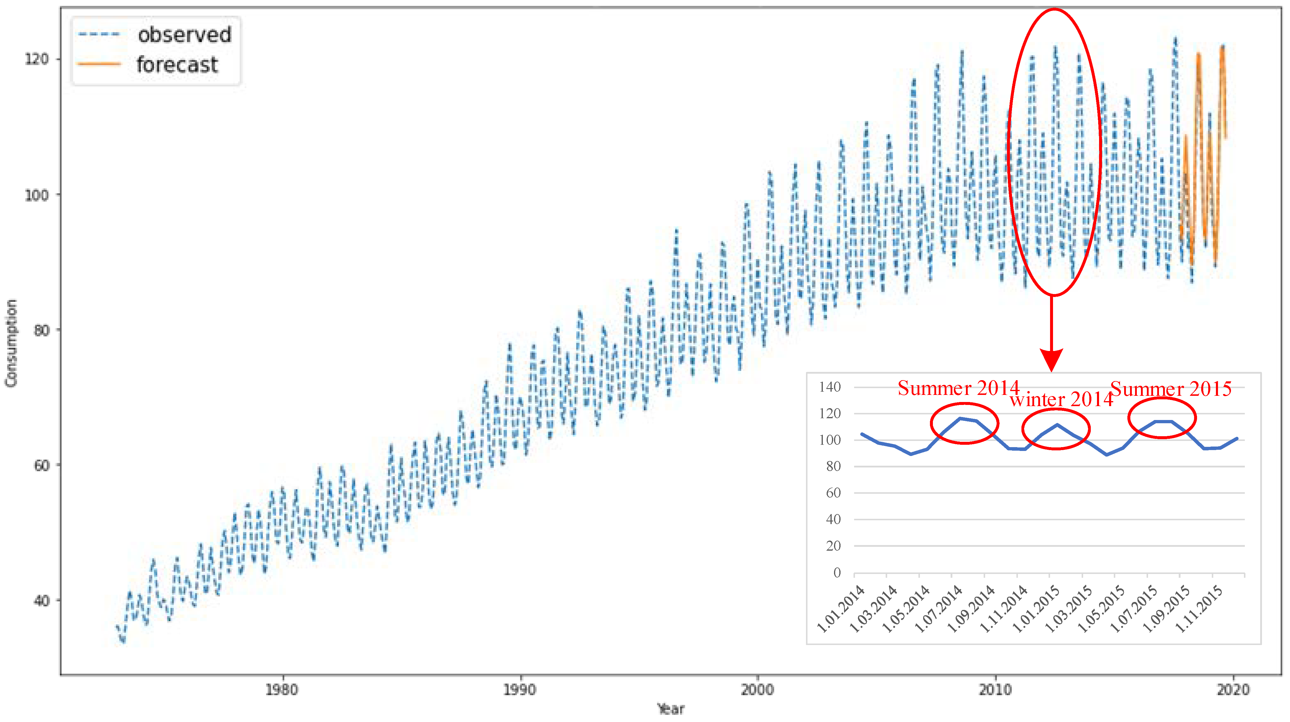
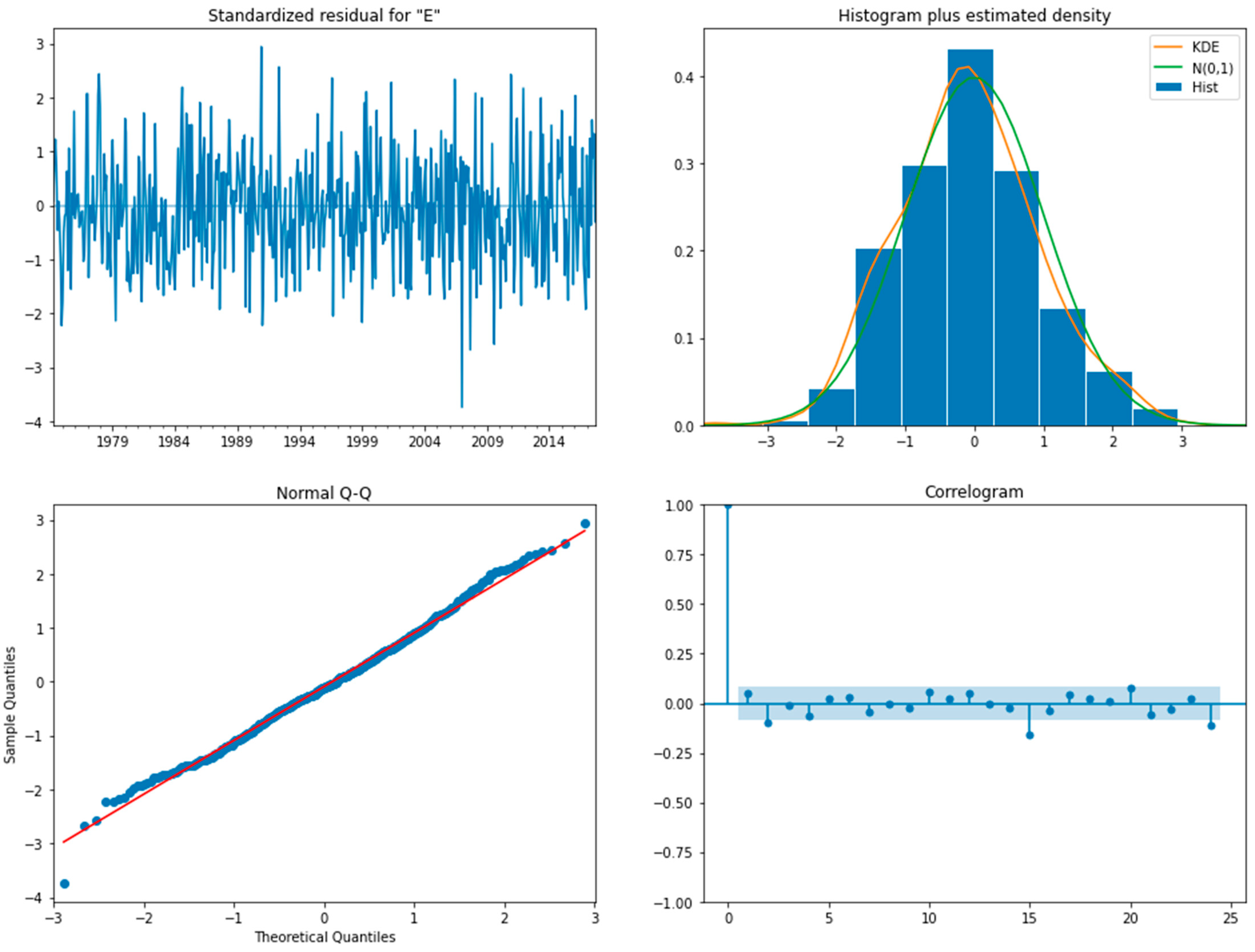
3.2. SARIMA Model Results
4. Discussion
4.1. Model Analysis
4.2. Implications for Energy Sector Planning
4.3. Consumer and Industry Impact
4.4. Continuous Monitoring and Adaptation
4.5. Limitations
4.6. Future Research Directions
5. Conclusions
Supplementary Materials
Author Contributions
Funding
Data Availability Statement
Conflicts of Interest
References
- Jose, R.; Panigrahi, S.K.; Patil, R.A.; Fernando, Y.; Ramakrishna, S. Artificial Intelligence-Driven Circular Economy as a Key Enabler for Sustainable Energy Management. Mater. Circ. Econ. 2020, 2, 8. [Google Scholar] [CrossRef]
- Zhou, Y. Sustainable energy sharing districts with electrochemical battery degradation in design, planning, operation and multi-objective optimisation. Renew Energy 2023, 202, 1324–1341. [Google Scholar] [CrossRef]
- Tajjour, S.; Chandel, S.S. A comprehensive review on sustainable energy management systems for optimal operation of future-generation of solar microgrids. Sustain. Energy Technol. Assess. 2023, 58, 103377. [Google Scholar] [CrossRef]
- Ozili, P.K.; Iorember, P.T. Financial stability and sustainable development. Int. J. Financ. Econ. 2023, ijfe.2803. [Google Scholar] [CrossRef]
- Opeyemi, B.M. Path to sustainable energy consumption: The possibility of substituting renewable energy for non-renewable energy. Energy 2021, 228, 120519. [Google Scholar] [CrossRef]
- Nguyen, X.P.; Le, N.D.; Pham, V.V.; Huynh, T.T.; Dong, V.H.; Hoang, A.T. Mission, challenges, and prospects of renewable energy development in Vietnam. Energy Sources Part A Recovery Util. Environ. Eff. 2021, 1–13. [Google Scholar] [CrossRef]
- Gunnarsdottir, I.; Davidsdottir, B.; Worrell, E.; Sigurgeirsdottir, S. Sustainable energy development: History of the concept and emerging themes. Renew. Sustain. Energy Rev. 2021, 141, 110770. [Google Scholar] [CrossRef]
- Holden, E.; Linnerud, K.; Rygg, B.J. A review of dominant sustainable energy narratives. Renew. Sustain. Energy Rev. 2021, 144, 110955. [Google Scholar] [CrossRef]
- Sovacool, B.K.; Newell, P.; Carley, S.; Fanzo, J. Equity, technological innovation and sustainable behaviour in a low-carbon future. Nat. Hum. Behav. 2022, 6, 326–337. [Google Scholar] [CrossRef]
- Johnson, O.W.; Han, J.Y.C.; Knight, A.L.; Mortensen, S.; Aung, M.T.; Boyland, M.; Resurrección, B.P. Intersectionality and energy transitions: A review of gender, social equity and low-carbon energy. Energy Res. Soc. Sci. 2020, 70, 101774. [Google Scholar] [CrossRef]
- Godil, D.I.; Sharif, A.; Rafique, S.; Jermsittiparsert, K. The asymmetric effect of tourism, financial development, and globalization on ecological footprint in Turkey. Environ. Sci. Pollut. Res. 2020, 27, 40109–40120. [Google Scholar] [CrossRef] [PubMed]
- Agyekum, E.B. Energy poverty in energy rich Ghana: A SWOT analytical approach for the development of Ghana’s renewable energy. Sustain. Energy Technol. Assess. 2020, 40, 100760. [Google Scholar] [CrossRef]
- Kabeyi, M.J.B.; Olanrewaju, O.A. Sustainable Energy Transition for Renewable and Low Carbon Grid Electricity Generation and Supply. Front. Energy Res. 2022, 9. Available online: https://www.frontiersin.org/articles/10.3389/fenrg.2021.743114 (accessed on 14 February 2024). [CrossRef]
- Devaraj, J.; Elavarasan, R.M.; Shafiullah, G.; Jamal, T.; Khan, I. A holistic review on energy forecasting using big data and deep learning models. Int. J. Energy Res. 2021, 45, 13489–13530. [Google Scholar] [CrossRef]
- Dong, Z.; Liu, J.; Liu, B.; Li, K.; Li, X. Hourly energy consumption prediction of an office building based on ensemble learning and energy consumption pattern classification. Energy Build. 2021, 241, 110929. [Google Scholar] [CrossRef]
- De Brauwer, C.P.-S.; Cohen, J.J. Analysing the potential of citizen-financed community renewable energy to drive Europe’s low-carbon energy transition. Renew. Sustain. Energy Rev. 2020, 133, 110300. [Google Scholar] [CrossRef]
- Sovacool, B.K.; Griffiths, S. Culture and low-carbon energy transitions. Nat. Sustain. 2020, 3, 685–693. [Google Scholar] [CrossRef]
- Inkulu, A.K.; Bahubalendruni, M.V.A.R.; Dara, A.; SankaranarayanaSamy, K. Challenges and opportunities in human robot collaboration context of Industry 4.0—A state of the art review. Industrial Robot 2022, 49, 226–239. [Google Scholar] [CrossRef]
- Nepal, B.; Yamaha, M.; Yokoe, A.; Yamaji, T. Electricity load forecasting using clustering and ARIMA model for energy management in buildings. Jpn. Archit. Rev. 2020, 3, 62–76. [Google Scholar] [CrossRef]
- Drame, M.; Seck, D.A.N.; Ndiaye, B.S. Analysis and Forecast of Energy Demand in Senegal with a SARIMA Model and an LSTM Neural Network. In The 4th Joint International Conference on Deep Learning, Big Data and Blockchain (DBB 2023); Younas, M., Awan, I., Benbernou, S., Petcu, D., Eds.; Springer Nature: Cham, Switzerland, 2023; Volume 768, pp. 129–140. [Google Scholar] [CrossRef]
- Rudnik, K.; Hnydiuk-Stefan, A.; Li, Z.; Ma, Z. Short-term modeling of carbon price based on fuel and energy determinants in EU ETS. J. Clean Prod. 2023, 417, 137970. [Google Scholar] [CrossRef]
- Kao, Y.-S.; Nawata, K.; Huang, C.-Y. Predicting Primary Energy Consumption Using Hybrid ARIMA and GA-SVR Based on EEMD Decomposition. Mathematics 2020, 8, 1722. [Google Scholar] [CrossRef]
- Elsaraiti, M.; Ali, G.; Musbah, H.; Merabet, A.; Little, T. Time Series Analysis of Electricity Consumption Forecasting Using ARIMA Model. In Proceedings of the 2021 IEEE Green Technologies Conference (GreenTech), Denver, CO, USA, 7–9 April 2021; IEEE: Piscataway, NJ, USA, 2021; pp. 259–262. [Google Scholar] [CrossRef]
- Babu, M.K.; Ray, P.; Sahoo, A.K. Cost and Energy Efficiency Study of an ARIMA Forecast Model Using HOMER Pro. In Recent Advances in Power Systems; Gupta, O.H., Singh, S.N., Malik, O.P., Eds.; Springer Nature: Singapore, 2023; Volume 960, pp. 137–151. [Google Scholar] [CrossRef]
- Ngo, N.-T.; Pham, A.-D.; Truong, N.-S.; Truong, T.T.H.; Huynh, N.-T. Hybrid Machine Learning for Time-Series Energy Data for Enhancing Energy Efficiency in Buildings. In Computational Science—ICCS 2021; Paszynski, M., Kranzlmüller, D., Krzhizhanovskaya, V.V., Dongarra, J.J., Sloot, P.M.A., Eds.; Springer International Publishing: Cham, Switzerland, 2021; Volume 12746, pp. 273–285. [Google Scholar] [CrossRef]
- Dubey, A.K.; Kumar, A.; García-Díaz, V.; Sharma, A.K.; Kanhaiya, K. Study and analysis of SARIMA and LSTM in forecasting time series data. Sustain. Energy Technol. Assess. 2021, 47, 101474. [Google Scholar] [CrossRef]
- Bilgili, M.; Pinar, E. Gross electricity consumption forecasting using LSTM and SARIMA approaches: A case study of Türkiye. Energy 2023, 284, 128575. [Google Scholar] [CrossRef]
- Bozkurt, Ö.Ö.; Biricik, G.; Tayşi, Z.C. Artificial neural network and SARIMA based models for power load forecasting in Turkish electricity market. PLoS ONE 2017, 12, e0175915. [Google Scholar] [CrossRef] [PubMed]
- Liu, X.; Lin, Z.; Feng, Z. Short-term offshore wind speed forecast by seasonal ARIMA—A comparison against GRU and LSTM. Energy 2021, 227, 120492. [Google Scholar] [CrossRef]
- Al-Shaikh, H.; Rahman, M.A.; Zubair, A. Short-Term Electric Demand Forecasting for Power Systems using Similar Months Approach based SARIMA. In Proceedings of the 2019 IEEE International Conference on Power, Electrical, and Electronics and Industrial Applications (PEEIACON), Electrical, Dhaka, Bangladesh, 29 November–1 December 2019; IEEE: Piscataway, NJ, USA, 2019; pp. 122–126. [Google Scholar] [CrossRef]
- Andoh, P.Y.A.; Sekyere, C.K.K.; Mensah, L.D.; Dzebre, D.E.K. Forecasting Electricity Demand in Ghana with The Sarima Model. J. Appl. Eng. Technol. Sci. (JAETS) 2021, 3, 1–9. [Google Scholar] [CrossRef]
- Bayindir, R.; Irmak, E.; Colak, İ.; Bektas, A. Development of a real time energy monitoring platform. Int. J. Electr. Power Energy Syst. 2011, 33, 137–146. [Google Scholar] [CrossRef]
- Bayi, R.; Hossai, E.; Kabalci, E.; Bi, K.M.M. Investigation on North American Microgrid Facility. Int. J. Renew. Energy Res. 2015, 5, 558–574. [Google Scholar]
- Li, P.; Zhang, J.-S. A New Hybrid Method for China’s Energy Supply Security Forecasting Based on ARIMA and XGBoost. Energies 2018, 11, 1687. [Google Scholar] [CrossRef]
- Le, T.; Vo, M.T.; Vo, B.; Hwang, E.; Rho, S.; Baik, S.W. Improving Electric Energy Consumption Prediction Using CNN and Bi-LSTM. Appl. Sci. 2019, 9, 4237. [Google Scholar] [CrossRef]
- Xing, Y.; Li, Y.; Liu, W.; Li, W.; Meng, L.-X. Operation Energy Consumption Estimation Method of Electric Bus Based on CNN Time Series Prediction. Math. Probl. Eng. 2022, 2022, 6904387. [Google Scholar] [CrossRef]
- Fuadi, A.Z.; Haq, I.N.; Leksono, E. Support Vector Machine to Predict Electricity Consumption in the Energy Management Laboratory. J. Resti (Rekayasa Sist. Dan Teknol. Inf.) 2021, 5, 466–473. [Google Scholar] [CrossRef]
- Lin, Z.; Cheng, L.; Huang, G. Electricity Consumption Prediction Based on LSTM with Attention Mechanism. IEEJ Trans. Electr. Electron. Eng. 2020, 15, 556–562. [Google Scholar] [CrossRef]
- Li, S.; Sriver, R.L.; Miller, D.E. Skillful Prediction of UK Seasonal Energy Consumption Based on Surface Climate Information. Environ. Res. Lett. 2023, 18, 064007. [Google Scholar] [CrossRef]
- Singh, J.P.; Alam, O.; Yassine, A. Influence of Geodemographic Factors on Electricity Consumption and Forecasting Models. IEEE Access 2022, 10, 70456–70466. [Google Scholar] [CrossRef]
- Srivastava, S. Causal Relationship between Electricity Consumption and GDP: Plausible Explanation on Previously Found Inconsistent Conclusions for India. Theor. Econ. Lett. 2016, 6, 276. [Google Scholar] [CrossRef]
- Soyler, I.; Izgi, E. Electricity Demand Forecasting of Hospital Buildings in Istanbul. Sustainability 2022, 14, 8187. [Google Scholar] [CrossRef]
- To, W.M.; Lee, P.K.C.; Lai, T.M. Modeling of Monthly Residential and Commercial Electricity Consumption Using Nonlinear Seasonal Models—The Case of Hong Kong. Energies 2017, 10, 885. [Google Scholar] [CrossRef]
- Presekal, A.; Herdiansyah, H.; Harwahyu, R.; Suwartha, N.; Sari, R.F. Evaluation of Electricity Consumption and Carbon Footprint of UI GreenMetric Participating Universities Using Regression Analysis. In E3s Web of Conferences; EDP Sciences: Ulys, France, 2018. [Google Scholar] [CrossRef]
- Barua, A.M.; Goswami, P.K. A Survey on Electric Power Consumption Prediction Techniques. Int. J. Eng. Res. Technol. 2020, 13, 2568–2575. [Google Scholar] [CrossRef]
- Zhang, Y.; Li, Q. A Regressive Convolution Neural Network and Support Vector Regression Model for Electricity Consumption Forecasting. In Advances in Information and Communication, Proceedings of the 2019 Future of Information and Communication Conference (FICC), San Francisco, CA, USA, 14–15 March 2019; Springer International Publishing: Berlin/Heidelberg, Germany, 2019. [Google Scholar] [CrossRef]
- Shan, S.; Cao, B.; Wu, Z. Forecasting the Short-Term Electricity Consumption of Building Using a Novel Ensemble Model. IEEE Access 2019, 7, 88093–88106. [Google Scholar] [CrossRef]
- Zhu, G.; Sha, P.; Lao, Y.; Su, Q.; Sun, Q. Short-Term Electricity Consumption Forecasting Based on the EMD-Fbprophet-LSTM Method. Math. Probl. Eng. 2021, 2021, 6613604. [Google Scholar] [CrossRef]
- Poudel, P. Data on Energy by Our World in Data: World Energy Consumption. Available online: https://www.kaggle.com/datasets/pralabhpoudel/world-energy-consumption (accessed on 20 December 2023).
- Lai, Y.; Dzombak, D.A. Use of the Autoregressive Integrated Moving Average (ARIMA) Model to Forecast Near-Term Regional Temperature and Precipitation. Weather. Forecast. 2020, 35, 959–976. [Google Scholar] [CrossRef]
- Schaffer, A.L.; Dobbins, T.A.; Pearson, S.A. Interrupted time series analysis using autoregressive integrated moving average (ARIMA) models: A guide for evaluating large-scale health interventions. BMC Med. Res. Methodol. 2021, 21, 58. [Google Scholar] [CrossRef] [PubMed]
- ArunKumar, K.E.; Kalaga, D.V.; Kumar, C.M.S.; Kawaji, M.; Brenza, T.M. Comparative analysis of Gated Recurrent Units (GRU), long Short-Term memory (LSTM) cells, autoregressive Integrated moving average (ARIMA), seasonal autoregressive Integrated moving average (SARIMA) for forecasting COVID-19 trends. Alex. Eng. J. 2022, 61, 7585–7603. [Google Scholar] [CrossRef]
- Singh, S.; Parmar, K.S.; Kumar, J.; Makkhan, S.J.S. Development of new hybrid model of discrete wavelet decomposition and autoregressive integrated moving average (ARIMA) models in application to one month forecast the casualties cases of COVID-19. Chaos Solitons Fractals 2020, 135, 109866. [Google Scholar] [CrossRef]
- ArunKumar, K.E.; Kalaga, D.V.; Kumar, C.M.S.; Chilkoor, G.; Kawaji, M.; Brenza, T.M. Forecasting the dynamics of cumulative COVID-19 cases (confirmed, recovered and deaths) for top-16 countries using statistical machine learning models: Auto-Regressive Integrated Moving Average (ARIMA) and Seasonal Auto-Regressive Integrated Moving Average (SARIMA). Appl. Soft Comput. 2021, 103, 107161. [Google Scholar] [CrossRef]
- Liu, H.; Li, C.; Shao, Y.; Zhang, X.; Zhai, Z.; Wang, X.; Qi, X.; Wang, J.; Hao, Y.; Wu, Q.; et al. Forecast of the trend in incidence of acute hemorrhagic conjunctivitis in China from 2011–2019 using the Seasonal Autoregressive Integrated Moving Average (SARIMA) and Exponential Smoothing (ETS) models. J. Infect. Public Health 2020, 13, 287–294. [Google Scholar] [CrossRef]
- Rabbani, M.B.A.; Musarat, M.A.; Alaloul, W.S.; Rabbani, M.S.; Maqsoom, A.; Ayub, S.; Bukhari, H.; Altaf, M. A Comparison Between Seasonal Autoregressive Integrated Moving Average (SARIMA) and Exponential Smoothing (ES) Based on Time Series Model for Forecasting Road Accidents. Arab. J. Sci. Eng. 2021, 46, 11113–11138. [Google Scholar] [CrossRef]
- Zhang, W.; Lin, Z.; Liu, X. Short-term offshore wind power forecasting—A hybrid model based on Discrete Wavelet Transform (DWT), Seasonal Autoregressive Integrated Moving Average (SARIMA), and deep-learning-based Long Short-Term Memory (LSTM). Renew Energy 2022, 185, 611–628. [Google Scholar] [CrossRef]
- Ray, S.; Das, S.S.; Mishra, P.; Al Khatib, A.M.G. Time Series SARIMA Modelling and Forecasting of Monthly Rainfall and Temperature in the South Asian Countries. Earth Syst. Environ. 2021, 5, 531–546. [Google Scholar] [CrossRef]
- Arlt, J.; Trcka, P. Automatic SARIMA modeling and forecast accuracy. Commun. Stat. Simul. Comput. 2021, 50, 2949–2970. [Google Scholar] [CrossRef]
- Adams, S.; Bamanga, M. Modelling and Forecasting Seasonal Behavior of Rainfall in Abuja, Nigeria; A SARIMA Approach. Am. J. Math. Stat. 2020, 10, 10–19. [Google Scholar] [CrossRef]
- Dimri, T.; Ahmad, S.; Sharif, M. Time series analysis of climate variables using seasonal ARIMA approach. J. Earth Syst. Sci. 2020, 129, 149. [Google Scholar] [CrossRef]
- Yilmaz, E.N.; Polat, H.; Oyucu, S.; Aksoz, A.; Saygin, A. Data storage in smart grid systems. In Proceedings of the 2018 6th International Istanbul Smart Grids and Cities Congress and Fair (ICSG), Istanbul, Turkey, 25–26 April 2018; IEEE: Piscataway, NJ, USA, 2018; pp. 110–113. [Google Scholar] [CrossRef]
- Fan, Z.; Yan, Z.; Wen, S. Deep Learning and Artificial Intelligence in Sustainability: A Review of SDGs, Renewable Energy, and Environmental Health. Sustainability 2023, 15, 13493. [Google Scholar] [CrossRef]
- Sloboda, B.; Montgomery, D.C.; Jennings, C.L.; Kulahci, M. Introduction to Time Series Analysis and Forecasting; Wiley: Hoboken, NJ, USA, 2008; Volume 25, p. 446. ISBN 978-0-471-65397-4. [Google Scholar]
- Chen, C.; Hu, Y.; Karuppiah, M.; Kumar, P.M. Artificial intelligence on economic evaluation of energy efficiency and renewable energy technologies. Sustain. Energy Technol. Assess. 2021, 47, 101358. [Google Scholar] [CrossRef]
- Lerman, L.V.; Gerstlberger, W.; Lima, M.F.; Frank, A.G. How governments, universities, and companies contribute to renewable energy development? A municipal innovation policy perspective of the triple helix. Energy Res. Soc. Sci. 2021, 71, 101854. [Google Scholar] [CrossRef]
- Chaikumbung, M. Institutions and consumer preferences for renewable energy: A meta-regression analysis. Renew. Sustain. Energy Rev. 2021, 146, 111143. [Google Scholar] [CrossRef]
- Huebner, G.; Shipworth, D.; Hamilton, I.; Chalabi, Z.; Oreszczyn, T. Understanding electricity consumption: A comparative contribution of building factors, socio-demographics, appliances, behaviours and attitudes. Appl. Energy 2016, 177, 692–702. [Google Scholar] [CrossRef]
- Granger, C.W.J.; Pesaran, M.H. Economic and statistical measures of forecast accuracy. J. Forecast. 2000, 19, 537–560. [Google Scholar] [CrossRef]
- Hahn, H.; Meyer-Nieberg, S.; Pickl, S. Electric load forecasting methods: Tools for decision making. Eur. J. Oper. Res. 2009, 199, 902–907. [Google Scholar] [CrossRef]
- Tronchin, L.; Manfren, M.; Nastasi, B. Energy efficiency, demand side management and energy storage technologies—A critical analysis of possible paths of integration in the built environment. Renew. Sustain. Energy Rev. 2018, 95, 341–353. [Google Scholar] [CrossRef]
- Hobbs, B.F. Optimization methods for electric utility resource planning. Eur. J. Oper. Res. 1995, 83, 1–20. [Google Scholar] [CrossRef]
- Sarker, E.; Seyedmahmoudian, M.; Jamei, E.; Horan, B.; Stojcevski, A. Optimal management of home loads with renewable energy integration and demand response strategy. Energy 2020, 210, 118602. [Google Scholar] [CrossRef]
- Pina, A.; Silva, C.; Ferrão, P. The impact of demand side management strategies in the penetration of renewable electricity. Energy 2012, 41, 128–137. [Google Scholar] [CrossRef]
- Garfield, F.R. Measuring and Forecasting Consumption. J. Am. Stat. Assoc. 1946, 41, 322–333. [Google Scholar] [CrossRef]
- Alakeson, V.; Wilsdon, J. Digital sustainability in Europe. J. Ind. Ecol. 2002, 6, 10–12. [Google Scholar] [CrossRef]
- Rahman, H.; Selvarasan, I.; Begum, A.J. Short-term forecasting of total energy consumption for India-a black box based approach. Energies 2018, 11, 3442. [Google Scholar] [CrossRef]
- Moret, S.; Gironès, V.C.; Bierlaire, M.; Maréchal, F. Characterization of input uncertainties in strategic energy planning models. Appl. Energy 2017, 202, 597–617. [Google Scholar] [CrossRef]
- Drèze, J.H.; Modigliani, F. Consumption decisions under uncertainty. J. Econ. Theory 1972, 5, 459–486. [Google Scholar] [CrossRef]
- Arghira, N.; Ploix, S.; Fǎgǎrǎşan, I.; Iliescu, S.S. Forecasting energy consumption in dwellings. Adv. Intell. Syst. Comput. 2013, 187, 251–264. [Google Scholar] [CrossRef]
- Brandoni, C.; Polonara, F. The role of municipal energy planning in the regional energy-planning process. Energy 2012, 48, 323–338. [Google Scholar] [CrossRef]
- Brugger, H.; Eichhammer, W.; Mikova, N.; Dönitz, E. Energy Efficiency Vision 2050: How will new societal trends influence future energy demand in the European countries? Energy Policy 2021, 152, 112216. [Google Scholar] [CrossRef]
- Gajowniczek, K.; Zabkowski, T. Electricity forecasting on the individual household level enhanced based on activity patterns. PLoS ONE 2017, 12, e0174098. [Google Scholar] [CrossRef] [PubMed]
- Sousa, J.L.; Martins, A.G.; Jorge, H. Dealing with the paradox of energy efficiency promotion by electric utilities. Energy 2013, 57, 251–258. [Google Scholar] [CrossRef][Green Version]
- Stern, P.C. Information, incentives, and proenvironmental consumer behavior. J. Consum. Policy 1999, 22, 461–478. [Google Scholar] [CrossRef]
- Hankinson, G.A.; Rhys, J.M.W. Electricity consumption, electricity intensity and industrial structure. Energy Econ. 1983, 5, 146–152. [Google Scholar] [CrossRef]
- Suganthi, L.; Samuel, A.A. Energy models for demand forecasting—A review. Renew. Sustain. Energy Rev. 2012, 16, 1223–1240. [Google Scholar] [CrossRef]
- Kaur, A.; Nonnenmacher, L.; Pedro, H.T.C.; Coimbra, C.F.M. Benefits of solar forecasting for energy imbalance markets. Renew. Energy 2016, 86, 819–830. [Google Scholar] [CrossRef]
- Przepiorka, W.; Horne, C. How Can Consumer Trust in Energy Utilities be Increased? The Effectiveness of Prosocial, Proenvironmental, and Service-Oriented Investments as Signals of Trustworthiness. Organ. Environ. 2020, 33, 262–284. [Google Scholar] [CrossRef]
- Rausser, G.; Strielkowski, W.; Mentel, G. Consumer Attitudes toward Energy Reduction and Changing Energy Consumption Behaviors. Energies 2023, 16, 1478. [Google Scholar] [CrossRef]
- Auffhammer, M.; Mansur, E.T. Measuring climatic impacts on energy consumption: A review of the empirical literature. Energy Econ. 2014, 46, 522–530. [Google Scholar] [CrossRef]
- Li, J.; Yang, L.; Long, H. Climatic impacts on energy consumption: Intensive and extensive margins. Energy Econ. 2018, 71, 332–343. [Google Scholar] [CrossRef]
- Li, D.H.W.; Yang, L.; Lam, J.C. Impact of climate change on energy use in the built environment in different climate zones—A review. Energy 2012, 42, 103–112. [Google Scholar] [CrossRef]
- York, R. Energy consumption trends across the globe. In Oxford Handbook of Energy and Society; Oxford University Press: Oxford, UK, 2018. [Google Scholar] [CrossRef]
- Kober, T.; Schiffer, H.W.; Densing, M.; Panos, E. Global energy perspectives to 2060—WEC’s World Energy Scenarios 2019. Energy Strategy Rev. 2020, 31, 100523. [Google Scholar] [CrossRef]
- Bollino, C.A.; Asdrubali, F.; Polinori, P.; Bigerna, S.; Micheli, S.; Guattari, C.; Rotili, A. A note on medium- and long-term global energy prospects and scenarios. Sustainability 2017, 9, 833. [Google Scholar] [CrossRef]
- Lin, B.; Su, T. Does COVID-19 open a Pandora’s box of changing the connectedness in energy commodities? Res. Int. Bus. Financ. 2021, 56, 101360. [Google Scholar] [CrossRef] [PubMed]
- Danish; Saud, S.; Baloch, M.A.; Lodhi, R.N. The nexus between energy consumption and financial development: Estimating the role of globalization in Next-11 countries. Environ. Sci. Pollut. Res. 2018, 25, 18651–18661. [Google Scholar] [CrossRef] [PubMed]
- Shahbaz, M.; Topcu, B.A.; Sarıgül, S.S.; Vo, X.V. The effect of financial development on renewable energy demand: The case of developing countries. Renew Energy 2021, 178, 1370–1380. [Google Scholar] [CrossRef]
- Lorente, D.B.; Álvarez-Herranz, A. Economic growth and energy regulation in the environmental Kuznets curve. Environ. Sci. Pollut. Res. 2016, 23, 16478–16494. [Google Scholar] [CrossRef]
- Liu, Y.; Li, Z.; Yin, X. Environmental regulation, technological innovation and energy consumption—A cross-region analysis in China. J. Clean. Prod. 2018, 203, 885–897. [Google Scholar] [CrossRef]
- Aydin, E.; Brounen, D. The impact of policy on residential energy consumption. Energy 2019, 169, 115–129. [Google Scholar] [CrossRef]
- Madlener, R.; Sunak, Y. Impacts of urbanization on urban structures and energy demand: What can we learn for urban energy planning and urbanization management? Sustain. Cities Soc. 2011, 1, 45–53. [Google Scholar] [CrossRef]
- Yang, J.; Ma, T.; Ma, K.; Yang, B.; Guerrero, J.M.; Liu, Z. Trading mechanism and pricing strategy of integrated energy systems based on credit rating and Bayesian game. Energy 2021, 232, 120948. [Google Scholar] [CrossRef]
- Hearne, C.J.; Makridakis, S.; Wheelwright, S.C. Forecasting Methods for Management. J. Oper. Res. Soc. 1991, 42. [Google Scholar] [CrossRef]
- Lynham, J.; Nitta, K.; Saijo, T.; Tarui, N. Why does real-time information reduce energy consumption? Energy Econ. 2016, 54, 173–181. [Google Scholar] [CrossRef]


| Model | ACF | PACF |
|---|---|---|
| MA(q) | Cuts off after lag q | Exponential decay and/or damped sinusoid |
| AR (p) | Exponential decay and/or damped sinusoid | Cuts off after lag p |
| ARMA (p,q) | Exponential decay and/or damped sinusoid | Exponential decay and/or damped sinusoid |
| Electricity_Consumption_in_TW | Month | Year |
|---|---|---|
| 35.9728 | 1 | 1973 |
| 36.1334 | 2 | 1973 |
| 35.0625 | 3 | 1973 |
| 33.8416 | 5 | 1973 |
| 33.5107 | 6 | 1973 |
| … | … | … |
| Dependent Variables | Electricity Consumption in TW | Number of Observations | 537 |
|---|---|---|---|
| Model | Exponential Smoothing | SSE | 0.469 |
| Optimized | Yes | AIC | −3749.979 |
| Trend | Multiplicative | BIC | −3681.403 |
| Seasonal period | 12 months | AICC | −3748.658 |
| Dependent Variables | Electricity Consumption in TW | Number of Observations | 537 |
|---|---|---|---|
| Model | SARIMAX (1,1,1) × (1,0,1,12) | Log-likelihood | 1289.004 |
| Sample | 01-01-1973 | AIC | −2568.009 |
| 01-09-2016 | BIC | −2546.720 | |
| Covariance Type | the outer product of gradients | HQIC | −2559.670 |
Disclaimer/Publisher’s Note: The statements, opinions and data contained in all publications are solely those of the individual author(s) and contributor(s) and not of MDPI and/or the editor(s). MDPI and/or the editor(s) disclaim responsibility for any injury to people or property resulting from any ideas, methods, instructions or products referred to in the content. |
© 2024 by the authors. Licensee MDPI, Basel, Switzerland. This article is an open access article distributed under the terms and conditions of the Creative Commons Attribution (CC BY) license (https://creativecommons.org/licenses/by/4.0/).
Share and Cite
Durmus Senyapar, H.N.; Aksoz, A. Empowering Sustainability: A Consumer-Centric Analysis Based on Advanced Electricity Consumption Predictions. Sustainability 2024, 16, 2958. https://doi.org/10.3390/su16072958
Durmus Senyapar HN, Aksoz A. Empowering Sustainability: A Consumer-Centric Analysis Based on Advanced Electricity Consumption Predictions. Sustainability. 2024; 16(7):2958. https://doi.org/10.3390/su16072958
Chicago/Turabian StyleDurmus Senyapar, Hafize Nurgul, and Ahmet Aksoz. 2024. "Empowering Sustainability: A Consumer-Centric Analysis Based on Advanced Electricity Consumption Predictions" Sustainability 16, no. 7: 2958. https://doi.org/10.3390/su16072958
APA StyleDurmus Senyapar, H. N., & Aksoz, A. (2024). Empowering Sustainability: A Consumer-Centric Analysis Based on Advanced Electricity Consumption Predictions. Sustainability, 16(7), 2958. https://doi.org/10.3390/su16072958