1. Introduction
Land subsidence is a geologic process that occurs when the ground surface gradually lowers due to natural or man-made causes [
1]. As the process is complex and nonlinear, the results are unpredictable and can vary greatly from one location to another [
2]. The effects of subsidence can be far-reaching and include changes in the landscape, disruption of surface water drainage, and destruction of buildings and infrastructure. It can be caused by natural factors such as soil compaction, tectonic movements, dissolution processes, and subsurface water removal, or by human activities such as mining and construction [
3,
4,
5,
6,
7,
8]. The impacts and extents of the various contributing elements can vary significantly from one geological setting to the next and can have a significant impact on the overall scale of the process. It is an intricate and gradual process that must be understood thoroughly to accurately assess its potential consequences. With the acceleration of urbanization, surface building load has become an important factor that can induce land subsidence [
9,
10]. To ascertain the connection between the surface construction burden and land subsidence, it is necessary to examine their spatial distributions and evaluate their correlation at varying scales.
Scale involves spatial scale and temporal scale. Spatial scale refers to the unit of space used in the study of an object or phenomenon and the spatial scope of a phenomenon or process [
11]. Spatial scales in geography can be represented by granularity and magnitude. Granularity is the smallest distinguishable element in a geospatial environment. Magnitude refers to the range of objects in space [
12]. Because of the strong spatial heterogeneity in the spatial distribution of both the surface building load and the land subsidence rate, the spatial characteristics of these two, as well as their correlation, exist in different scales. As urbanization intensifies, the influence of surface buildings on land subsidence becomes increasingly prominent, making it imperative to assess their impact through varied spatial lenses. This approach is essential for comprehending the full scope and impact of land subsidence in diverse geological and urban environments.
Wavelet analysis is a multi-scale analytical method known as a mathematical microscope [
13]. Wavelet analysis is mainly used in signal denoising and information feature extraction. In recent years, wavelet analysis has been widely applied in the fields of photogrammetry and remote sensing, deformation observation data analysis, and seismic signal analysis, and satisfactory results have been obtained [
14]. It is necessary to understand the spatial distribution characteristics of surface building load and land subsidence when using wavelet multistage decomposition. Moran’s I index measures the correlation of elements between adjacent positions in space, known as spatial autocorrelation [
15,
16].
The Beijing Plain area is currently grappling with a critical issue of land subsidence, posing a significant risk to the stability and safety of buildings and infrastructure in the region. Recognizing this threat, the Chinese government has initiated actions to curb groundwater extraction, a key factor contributing to this problem. However, to mitigate further subsidence effectively, additional strategies are required. In the context of Beijing, it has been identified that the primary factors influencing land subsidence are the thickness of compressible deposits and groundwater levels, highlighting the critical need for integrated management of geological conditions and water resources [
17]. The rapid urbanization of Beijing, marked by extensive construction of new buildings, especially in the Tongzhou District where land subsidence is notably severe, has greatly exacerbated this environmental challenge [
18]. This has caused the ground to become compressed and has led to land subsidence. The increase in building construction in Beijing’s central region has led to a high building density, while the eastern regions of Chaoyang and Tongzhou experience a high rate of land subsidence. Building density is becoming a significant factor contributing to land subsidence.
1.1. Studies Analyzing Characteristics of Land Subsidence
Currently, point-based geodetic methods, such as geoid surveys and global navigation satellite systems, are commonly used for monitoring urban surface deformation, but these methods suffer from low spatial resolution and high cost. In contrast, the Persistent Scatterers Interferometric Synthetic Aperture Radar (PSInSAR) technique has been developed to attenuate incoherence due to long spacetime baselines and mitigate atmospheric and topographic effects on the difference, thereby improving the accuracy of InSAR monitoring [
19]. Many studies have demonstrated the applicability and reliability of PSInSAR techniques in vegetation cover areas and urban surface deformation monitoring. Nearly 300 high-resolution COSMO-SkyMed StripMap HIMAGE scenes were utilized to monitor the long-term subsidence process in Wuhan, proving the benefits of nonlinear PSInSAR in analyzing the temporal evolution of land subsidence in dynamic and expanding cities like Wuhan [
20]. Gonnuru et al. used advanced the PSInSAR technique to estimate land subsidence due to oil extraction in the Burgan oil field in Kuwait, and found a total subsidence of 10 mm/year and an average of 25–30 mm per 3 years, demonstrating the potential of PSInSAR for subsidence mapping in oil extraction areas [
21]. As we can conclude, PSInSAR has emerged as a primary method for monitoring large-scale land subsidence, demonstrating its effectiveness in various contexts, from urban surface deformation to vegetation cover areas and oil extraction fields, and overcoming the limitations of traditional geodetic methods in terms of spatial resolution and cost.
Existing research has primarily focused on the impact of urban expansion on land subsidence, with a particular emphasis on factors such as groundwater extraction and surface load conditions. This work includes global studies conducted in regions like China, Mexico, Spain, and the United States, revealing the significant role of these factors in inducing land subsidence. Numerous studies have shown that over-extraction of groundwater and the geological conditions are important driving factors for land subsidence in many parts of the world [
22]. In parts of China, Mexico, and the United States, extensive groundwater pumping for agriculture, industry, and urban water supplies has caused widespread land subsidence. Budihardjo et al. extended the knowledge of footing subsidence causing by groundwater pumping by considering various well and load conditions [
23]. Zhou et al. investigated the land subsidence in the Beijing Plain over the period of 2003–2015 and discussed the relation between groundwater pumping and land subsidence [
17]. Yu et al. proposed a relationship for the physics and mechanics constants of porous media related to water storage rate and ground settlement under a surface load variation condition [
24]. Chen et al. investigated the spatial and temporal dynamics of land subsidence in the Beijing Plain and revealed the relationship between subsidence and the groundwater level drops in the main exploration aquifer layers were relatively high [
25]. The evolutionary characteristics of land subsidence and rebound in Xi’an from 2007 to 2019 was investigated, and their cause and the correlation with groundwater level changes and the underground space utilization were discussed [
26].
Studies have investigated various factors, both at the macro and micro scales, leading to land subsidence in rapidly urbanizing areas. These factors include urban expansion and the construction of large buildings, as well as smaller-scale factors such as changes in ground building volume. By identifying the causes of land subsidence, researchers can better understand the mechanisms driving this phenomenon and develop strategies to mitigate its impact. Wu et al. showed that the land deformation suffered two periods (from 2015 to 2017 and from 2017 to 2019) and expanded from urban centers to surrounding resettlement areas, which are highly relevant with the urban earthwork process [
27]. Based on the principle of a strategic environmental assessment (SEA) for sustainable urban development, Xu et al. presented a discussion and analysis of the factors which can influence the development of land subsidence during continued urbanization in Shanghai [
28]. However, the impact of building volume on land subsidence remained stable once the volume of buildings became larger than 3.00 × 10
5 m
3. Jiao et al. used advanced technologies like PSInSAR and SAR tomography for monitoring land subsidence and building height estimation in rapidly urbanizing areas, showing that the correlation between building volumes and land subsidence increased as the volume of buildings increased [
9].
In conclusion, while PSInSAR has emerged as a key tool in the broad-scale detection of land subsidence, it has also facilitated the understanding of its main causes, including the often-overlooked yet significant role of surface construction. The growing body of research underscores the need to integrate the effects of urban development and building density into the assessment and mitigation strategies for land subsidence, recognizing them as integral factors in the urban geologic dynamic.
1.2. Studies on the Relationship between Surface Buildings and Land Subsidence
Building on the insights from the previous sections, it becomes evident that surface buildings are an influential factor in land subsidence that cannot be overlooked. Recent studies on the relationship between surface buildings and land subsidence offer diverse perspectives. Wang et al. (2018) explored the impact of building load in Beijing, using Floor Area Ratio to reflect this load, and found a notable correlation with land subsidence, particularly in areas with high building concentration [
10]. Cui et al. focused on land subsidence due to high-rise buildings in soft soil areas like Shanghai and Tianjin and highlighted the significant effects of building load [
29]. Xu et al. reviewed the effects of urbanization on land subsidence in Shanghai, addressing factors including construction activities and groundwater level changes that relate to building density [
30]. Li et al. proposed a model integrating the effects of high-rise building load and groundwater withdrawal, recognizing the complex and nonlinear nature of their interaction on land subsidence [
31].
The cumulative research on surface buildings and their impact on land subsidence establishes that building load indeed influences ground subsidence. Previous studies have primarily analyzed this relationship from the perspective of building load, focusing on the weight and structural impact of buildings. However, building density offers a different yet equally important angle. It reflects the concentration or clustering of buildings in an area which can create an equivalent load effect. This concentration can influence subsidence patterns, possibly in ways distinct from the impact of individual building loads.
1.3. Studies on Multi-Scale Geoprocessing Analyses Using Wavelet Transform
Wavelet transform allows for the decomposition of a signal or image into multiple scales or frequency bands, which enables the extraction of both low-frequency and high-frequency information. This makes it particularly useful for analyzing complex geospatial data that may contain information at different spatial or temporal scales. Based on the characteristics of geoprocessing, the two components can be considered as noise and eliminated to enhance the image or improve the geoprocessing analysis.
Haze is distributed in the lower frequency layer of wavelet transform, which is a noise to be eliminated [
32]. He et al. applied wavelet denoising to remove the high-frequency component in forest resource management and monitoring to improve the accuracy of forest classification [
33]. Mirghasemi et al. introduced a Particle Swarm Optimization (PSO)-based feature enhancement approach in the wavelet domain for noisy image segmentation [
34]. Wavelet transform is used to abstract the information from both the high- and low-frequency components in remote sensing image fusion [
35].
Wavelet transform has been successfully used in various fields, including forest resource management, image segmentation, and remote sensing image fusion, by removing noise and enhancing features in different frequency layers. This capability of wavelet transform can also be applied to land subsidence analysis for abstracting information from both high- and low-frequency components. Miller et al. employed multitemporal synthetic aperture radar data sets acquired by European Remote-Sensing Satellites (ERSs) and Envisat satellites to investigate ground deformation and used continuous wavelet transform to decompose time-series land subsidence, proving the capability of wavelet transform in comparing the short-term signal components of hydraulic head and vertical land subsidence [
36]. Ikuemonisan et al. studied Sentinel-1-derived land subsidence using wavelet tools and a triple exponential smoothing algorithm in Lagos, Nigeria [
37].
In summary, there is a predominant focus on groundwater extraction and geological changes, with a notable oversight of the impacts of urban construction and building density. This gap is addressed in our study through a comprehensive analysis of the spatial distribution and interrelation between surface building load and land subsidence. Furthermore, we extend the scope beyond traditional macro-scale analyses by employing wavelet analysis, allowing for a nuanced examination of land subsidence impacts across varied spatial scales. In addition, our research integrates the critical aspects of rapid urbanization and extensive construction, factors that have been previously underrepresented in land subsidence assessments. Through this approach, our study offers a more holistic understanding of urban geological dynamics, addressing these identified gaps and contributing to a more effective and comprehensive approach to land subsidence evaluation and management.
To address this gap, our method introduces a novel approach. We first use PSInSAR technology to collect comprehensive land subsidence data. Then, through wavelet decomposition, we separate the high- and low-frequency components of these data, identifying the high-frequency component as noise and focusing on the more relevant low-frequency component for in-depth analysis.
Subsequently, we apply Moran’s I analysis to explore the spatial distribution characteristics of the high- and low-frequency components of land subsidence, as well as those of groundwater, clay layers, and surface building density. This enables us to discern and differentiate the impacts of each factor. Specifically, our method allows us to isolate the influences of groundwater and clay layer thickness, thereby clarifying the relationship between surface building density and land subsidence.
By implementing this approach, we provide a more nuanced understanding of the various factors contributing to land subsidence, especially highlighting the role of urban construction. This comprehensive analysis offers valuable insights for urban planning and environmental management, particularly in densely built-up areas.
2. Materials and Methods
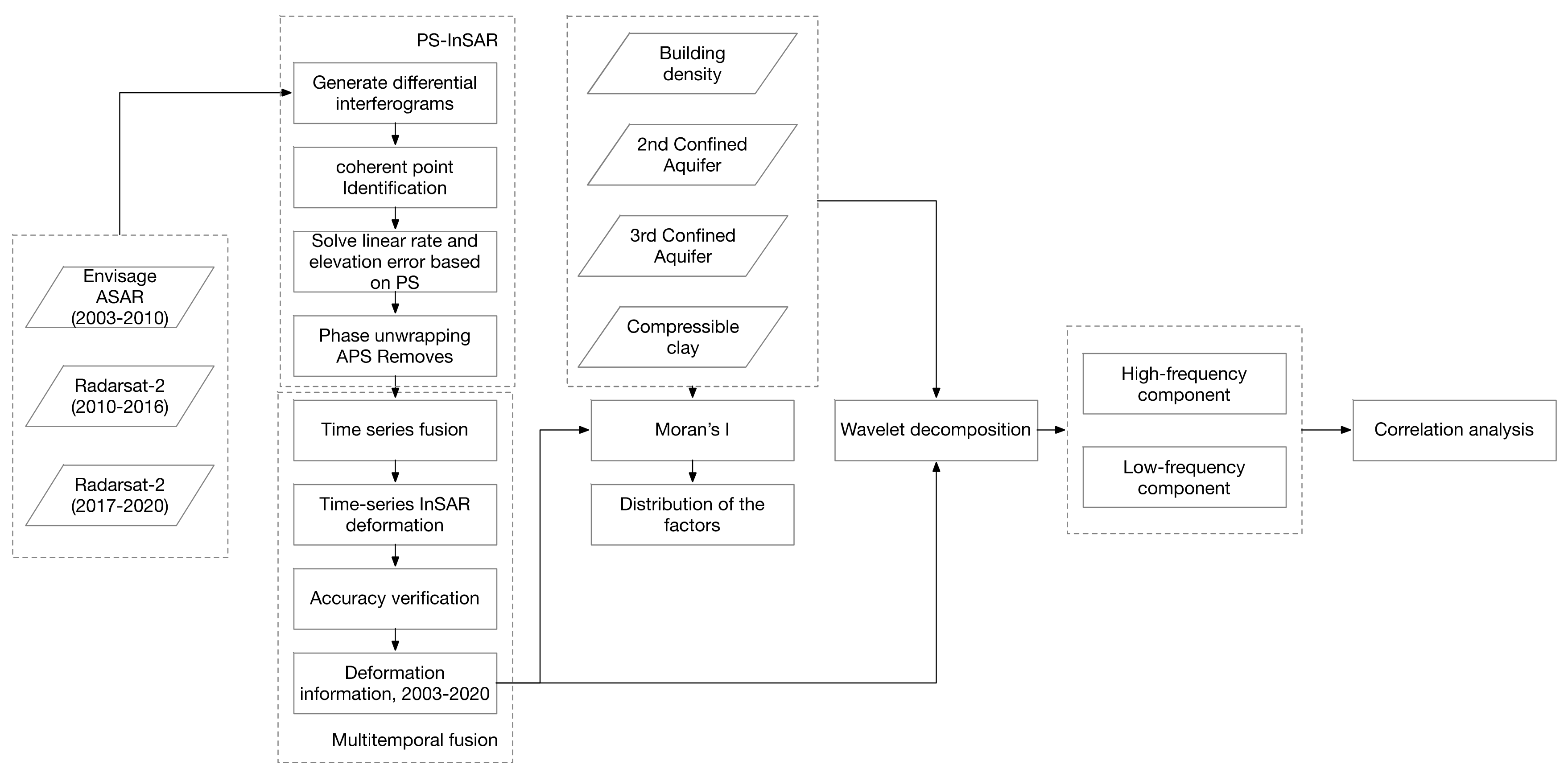
In this study, the Beijing Plain was identified as the primary area of focus, with its geographical, hydrogeological, and urban characteristics comprehensively outlined to provide a robust basis for analysis. PSInSAR technology was utilized to acquire InSAR imagery from various temporal periods, selected to effectively capture the dynamic progression of land subsidence over time. The resolution of these images was meticulously chosen to ensure both the precision and depth of the subsidence analysis. The Moran’s I index was applied to examine the spatial distribution of critical factors affecting land subsidence, such as groundwater levels, clay layer thickness, and urban infrastructure density. This step was succeeded by the acquisition of SAR data to integrate the extensive hydrogeological conditions of the Beijing Plain. Through wavelet decomposition, the land subsidence data were segmented into high-frequency and low-frequency components, facilitating a nuanced exploration of their correlations with groundwater, clay layer thickness, and building density. This methodological approach not only segregated the impacts of these variables but also enabled a comprehensive evaluation of urban infrastructure’s effect on land subsidence, as depicted in the main flow chart (
Figure 1).
2.1. Description of the Beijing Plain
Beijing is a huge metropolitan area as the political and cultural center of China, the population of which has been up to 20 million [
38]. Most people live in southeast of Beijing in the Beijing Plain. Beijing’s plain area is composed of water-bearing alluvial–pluvial and river channel deposits overlying bedrock. Tertiary and older sedimentary and volcanic rock units underlie quaternary sediments and form the lateral and basal boundaries of the aquifer system.
The shortage of water supply is a key issue for the city as groundwater extraction accounts for 2/3 of the total supply. The water consumption has been increasing to satisfy the requirement of the urban development, resulting in the overexploitation of groundwater. Since 1990, the relatively stable groundwater pumping rate has been about 2.5 × 10
9 m
3/year [
9]. The study by Chen et al. revealed a correlation between land subsidence and groundwater levels, noting that the geographic distribution of land subsidence often corresponds with areas of decreased groundwater, although not exclusively [
18].
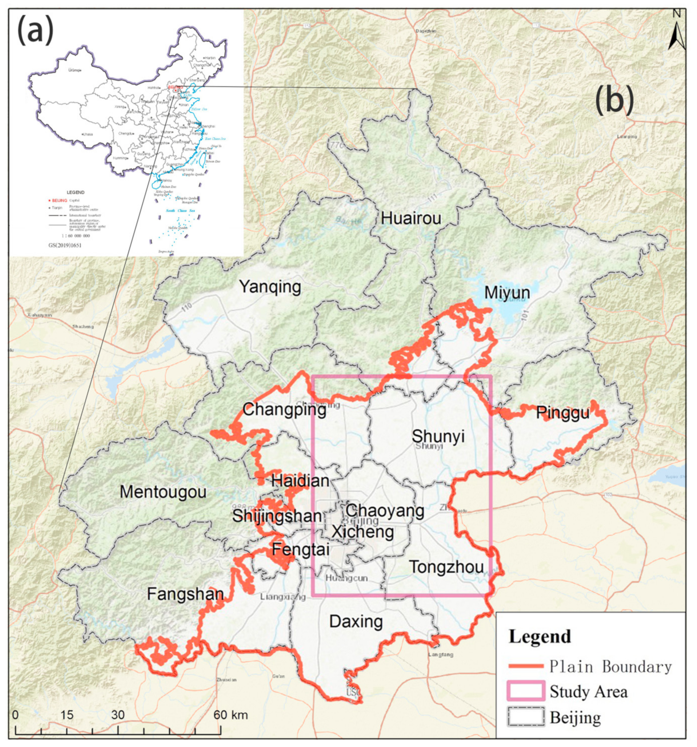
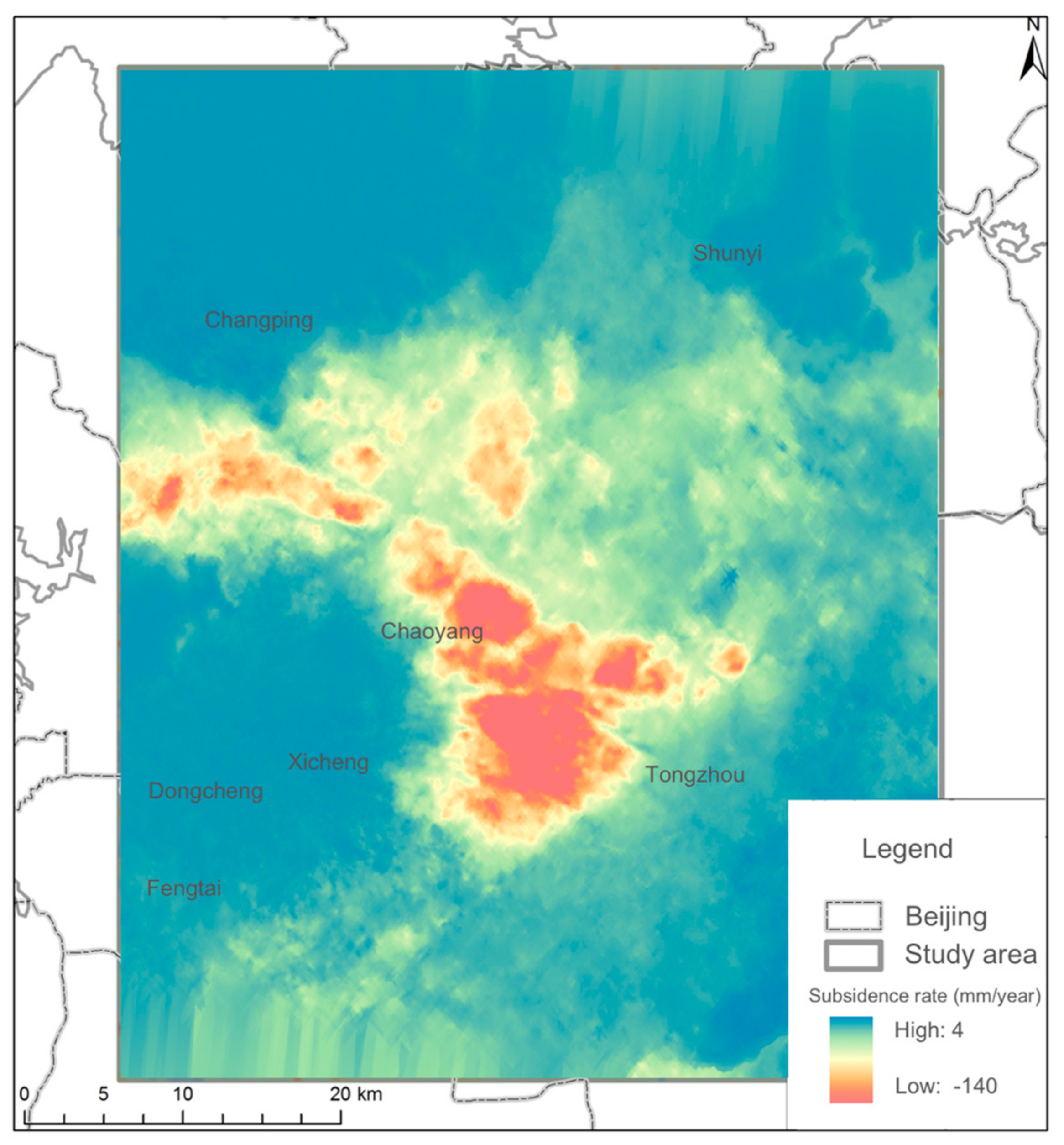
In recent decades, following the process of urbanization, the Chaoyang District has become the economic center of Beijing and the Tongzhou District has become a sleep city where there are residences. However, there is increasing land subsidence in this area, especially at the jointure of the Chaoyang and Tongzhou Districts, which is a high risk for urban security and will affect the common life of residences there. As shown in
Figure 2, the study site was located in a rectangular range of the Beijing Plain, including the entirety of Xicheng and Dongcheng, and parts of Changping, Chaoyang, Shunyi, Tongzhou, Daxing.
2.2. SAR Data Sets
The InSAR data used in this paper include Envisat ASAR data (2003.06.18~2010.09.19), Radarsat-2 data (2010.11.22~2016.10.21), and Radarsat-2 data (2017.01.25~2020.01.10), detailed in
Table 1. Among them, the Envisat satellite, launched by the European Space Agency on 1 March 2002, carries the synthetic aperture radar system ASAR, which supports around-the-clock operations and is widely used in the oceans, on the ground, and elsewhere. The SAR commercial satellite Radarsat-2 was launched on 14 December 2007 and can meet monitoring needs in the areas of oceans, the environment, disasters, sea ice, and others.
2.3. Hydrogeological Data
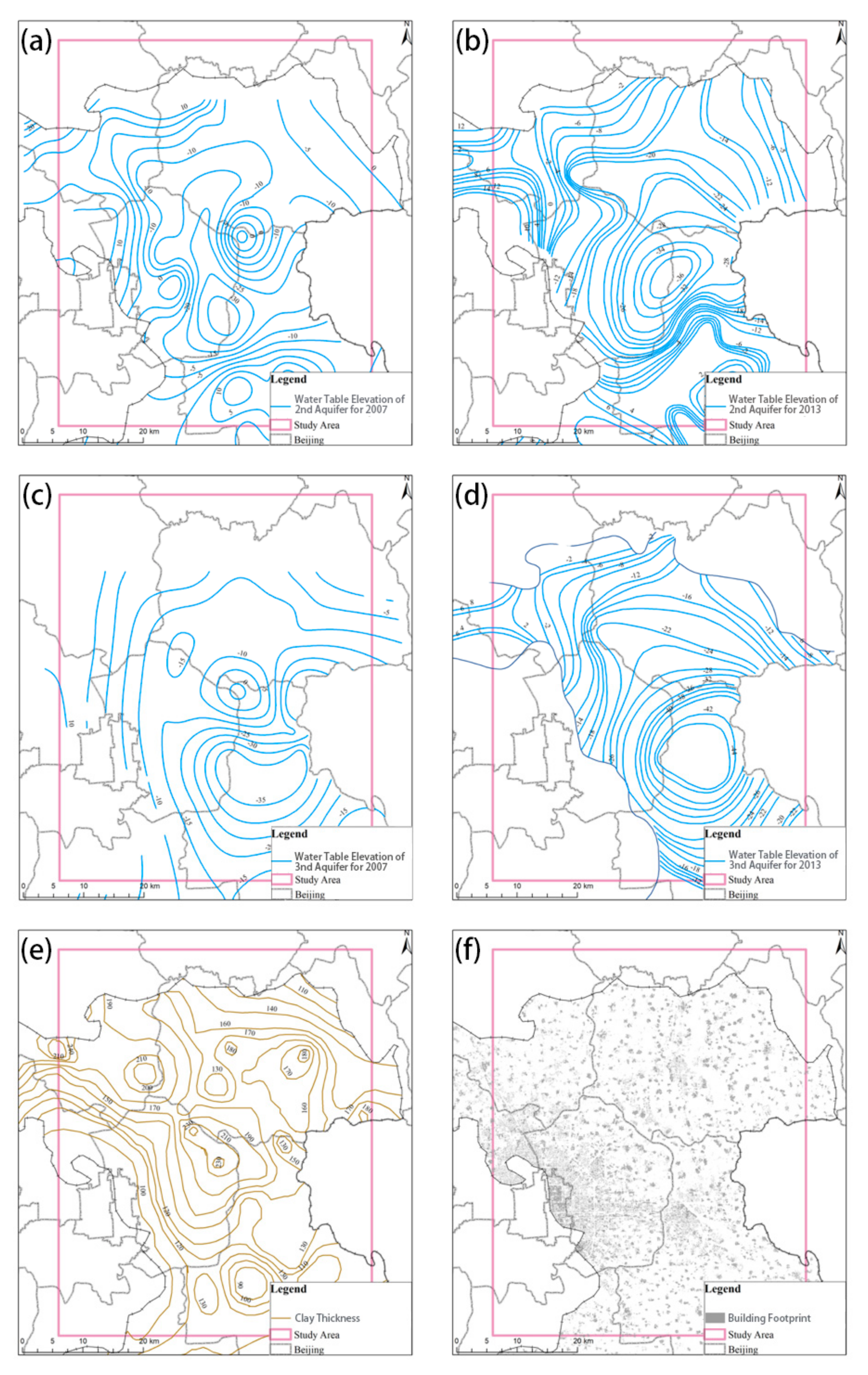
To investigate the primary factors influencing land subsidence, this study compiled key data elements. These included the water table elevations of the second confined aquifer for the years 2007 and 2013, as presented in
Figure 3a,b, and the water table elevations of the third confined aquifer for the same years, illustrated in
Figure 3c,d. Additionally, data on the thickness of compressible clay from the year 2005, sourced from earlier research, are shown in
Figure 3e. By integrating these data sets, our study aims to offer a comprehensive analysis of the spatial distribution of key factors contributing to land subsidence. This multidisciplinary approach allows us to not only identify the primary drivers of subsidence, but also to understand their spatial heterogeneity across the study area. Furthermore, to estimate the impact of land subsidence considering the impact of building density, we collected the building footprint of the Beijing Plain to calculate the density of buildings. All potential factors of hazard indicators were drawn and interpolated to raster format in ArcMAP (
Figure 3f).
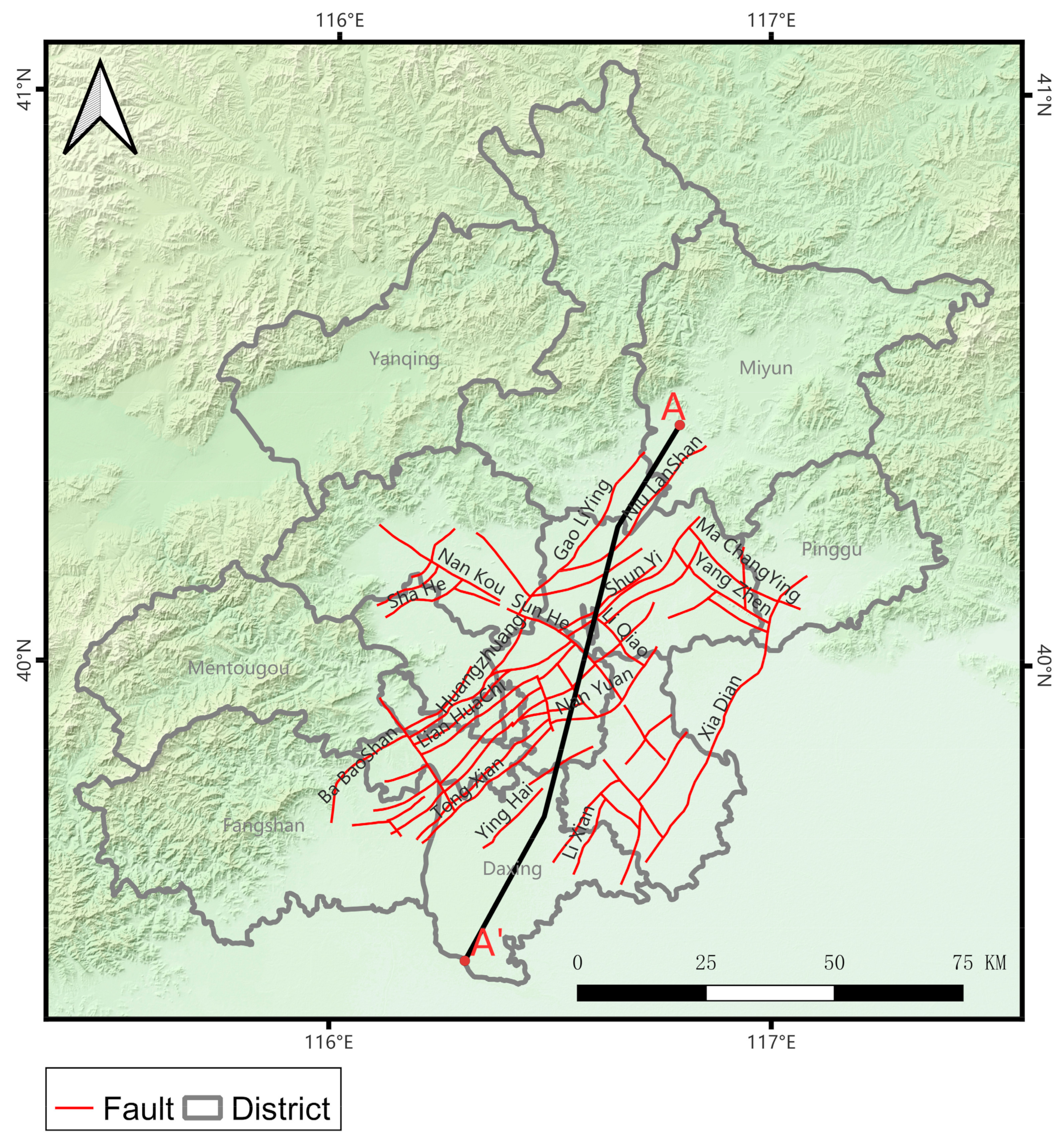
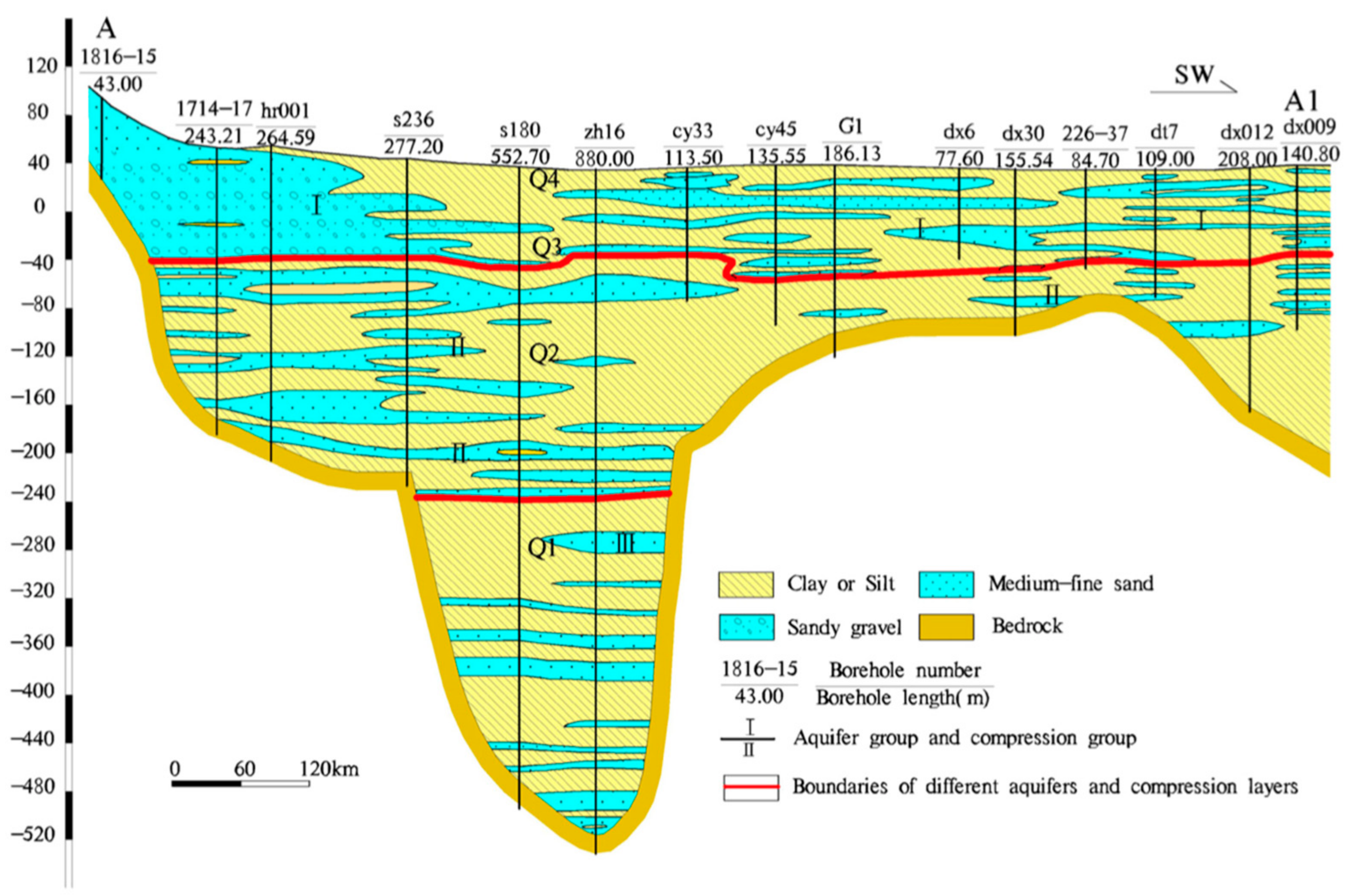
The Beijing Plain is traversed by multiple active high-angle faults (
Figure 4). Among them, the Nankou–Sunhe Fault is the largest northwest-oriented fault in Beijing, exhibiting both stick-slip and creep characteristics. The Huangzhuang–Gaoliying Fault, Liangxiang–Shunyi Fault, and Nanyuan–Tongxian Fault are southwest–northeast-oriented faults. The Huangzhuang–Gaoliying Fault is the largest northeast-oriented fault in Beijing and is characterized by significant segmented activity. Moreover, the Beijing Plain’s stratigraphy exhibits a clear division in terms of the quaternary sedimentary characteristics, crucial for understanding its hydrogeological and soil properties shown in
Figure 5 [
39]. The first stratigraphic division comprises the Holocene (Q4) and Upper Pleistocene (Q3) layers. The aquifer within this division includes an unconfined and a shallow confined aquifer, with depths of approximately 25 m for Holocene deposits and 80 to 120 m for Upper Pleistocene deposits. The corresponding soil layer, prevalent across the Beijing Plain, is composed of Upper Pleistocene alluvial facies, alluvial silt, and cohesive soil, with depths not exceeding 100 m. In the second division, characterized by the Middle Pleistocene (Q2) strata, the aquifer displays a multi-layered structure, primarily consisting of medium-coarse sand and gravel and extending to a depth of about 300 m. The associated soil layer, predominantly located in the middle and lower parts of the Plain, includes Middle Pleistocene alluvial and lacustrine facies, silt, silty clay, and clay, with a maximum depth of 300 m. The third division aligns with the Lower Pleistocene (Q1) epoch, featuring a deep aquifer system primarily composed of medium-coarse sand and gravel situated above the basement rocks. The soil layer in this division, primarily found in central major sedimentary depressions, consists of Lower Pleistocene alluvial and lacustrine facies, silty clay, and clay, with a depth exceeding 300 m. This delineation of aquifers and soil profiles in the Beijing Plain provides a detailed framework for geological and hydrological analyses, highlighting the complex relationship between different sedimentary epochs and the subsurface hydrodynamic processes.
2.4. Persistent Scatterers Interferometry (PSI)
For long-term land subsidence monitoring we used two different image subsets, Envisat ASAR and Radarsat-2, by applying PSInSAR technology.
PSInSAR is proposed to effectively reduce the impact of spatial–temporal decoherence and the atmosphere delay on land subsidence monitoring. In the single master PSInSAR process, a master image should be selected as the first step and all the other images (K images) are coregistered to the master image. After the interference process, K interferograms are created. According to the coherence of each pixel of interferograms, permanent scatterers are selected for further analysis. Settlement can be estimated by the differential interference mode [
40]. The equation is shown below (Equation (1))
where
denotes the phase of
pixel in the
interferogram,
denotes the deformation phase along the sight of the radar,
denotes the phase caused by the atmosphere effect,
denotes the phase caused by the orbit error,
denotes the phase caused by the Digital Elevation Model (DEM) error, and
denotes the random noise.
In this paper, a PSInSAR-based method was used to process Envisat ASAR and Radarsat-2 data by GAMMA software (GAMMA 2017) to obtain line-of-sight land subsidence. Using ArcGIS software (ArcGIS Pro 3.0), the line-of-sight rate was converted to a vertical rate. Finally, the continuous surface deformation information of the Beijing Plain from 2003 to 2020 was obtained by a time series fusion method, which mainly includes subsidence rates and cumulative subsidence.
2.5. Space Heterogeneity, Space Autocorrelation, and Moran’s I
Spatial heterogeneity refers to spatial data distribution characteristics due to spatial location. The positive correlation above space means that the closer the spatial distribution position (distance) is, the more obvious the correlation between spatial data becomes. Negative correlation in space means that the more discrete the spatial distribution location, the more significant the spatial data correlation becomes. To analyze the correlation between building density and land subsidence, the distribution characteristics of building density space should be explored. The spatial autocorrelation is the main measure of spatial distribution characteristics of geographical elements. The spatial autocorrelation is divided into global spatial autocorrelation and local spatial autocorrelation.
The global autocorrelation analysis is usually used to study the spatial autocorrelation of building density throughout the region. The common measure is global Moran’s I (Equation (2)), which is calculated as follows:
where
N is the number of space units,
is the sentient variable,
is the mean of
,
is the spatial weight matrix, and
is the sum of all
.
Common weight matrices are adjacency weight matrices, distance weight matrices, and K-nearest weight matrices. In this paper, the local spatial characteristics of the building density of each basic unit were analyzed by taking the street office of the smallest administrative unit in Beijing as the basic unit. Distance weight matrix or adjacency weight matrix is often used to calculate the local Moran’s I index of surface data. Because the area of Beijing administrative units is different, the adoption of a distance weighting matrix would lead to the phenomenon of an “isolated island” or the number of neighbors, so this paper adopts the adjacency weighting matrix method.
2.6. Wavelet Transform Principles
Wavelet transform has unique advantages in processing non-stationary sequence data. Wavelet variation is a new time–frequency analysis method based on the Fourier transform proposed by Morlet et al. Since 1990, wavelet transform has been widely used in denoising and signal reconstruction.
The basic idea of wavelet transform is to approach a signal or function using a wavelet function. The multiresolution of wavelet transform can be used to effectively separate the components of different frequencies in the signal, and then reconstruct the signal with the wavelet coefficients [
41] to obtain valuable information. The wavelet function (Equation (3)) is defined as:
Wavelet multiresolution analysis decomposes the processed signal at different resolution levels with positive cross transform. Signals that exist at the higher level and disappear at the lower level are called detailed signals [
42], that is, the high-frequency part of the signal. Multiresolution analysis can be expressed as follows:
For any function, V
0 can be broken down into the detail part W
1 and the stable change part V
1. V
1 can be further decomposed using the Mallat algorithm (Equations (4) and (5)) to break down signals into different frequency components:
These wavelet decompositions can be written as:
When decomposed according to the Mallat algorithm, global and local information of the signal can be distinguished [
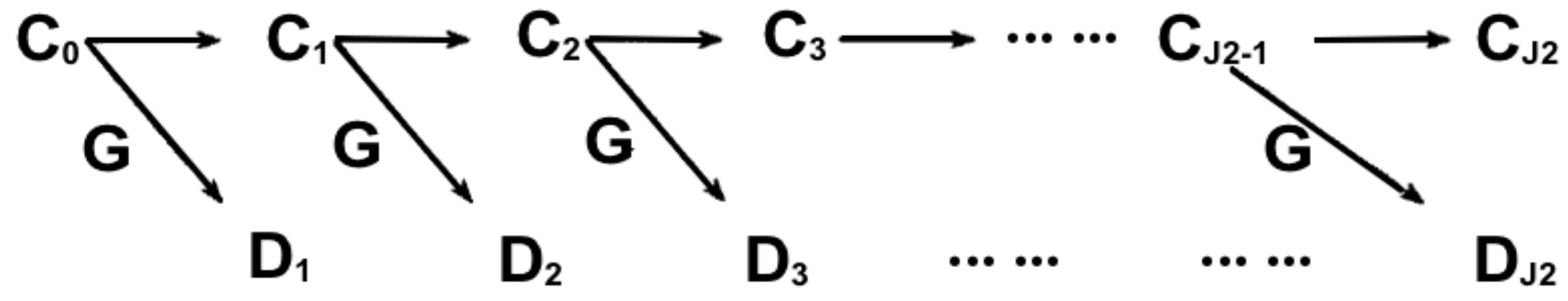
43]. Equations (6) and (7) are the Mallat Tower decomposition algorithms, as shown in
Figure 6. Starting with the initial signal
, the process iteratively bifurcates the signal into two distinct components at each level: a detail signal
and an approximation signal
. At each decomposition level, the detail signal
, containing the local (high-frequency) information of the signal, is extracted by applying a high-pass filter. Concurrently, the approximation signal
, representing the global (low-frequency) information, is obtained through a low-pass filter. In the context of the Mallat algorithm, these filtering processes are symbolized by the operations ‘G’ for smoothing and ‘D’ for detailing.
According to the Mallat algorithm, signals can be broken down into low-frequency and high-frequency segments.
To obtain the land subsidence information under different spatial granularities, the land subsidence rate grid image was obtained by Kriging interpolation of the land subsidence rate obtained by PSInSAR with the same spatial resolution as the ASAR image. The low-frequency coefficient of land subsidence information, which is the macroscopic area of Beijing land subsidence information, was obtained by decomposing the image into a four-level two-dimensional wavelet. And the high-frequency coefficient of land subsidence, which is the local detail characteristic of Beijing land subsidence, had low spatial autocorrelation, that is, random spatial distribution.
3. Results
3.1. Land Subsidence Rate
Based on 55 Scenario Envisat ASAR, 37 Scenario Radarsat-2 (2011–2016), and 43 Scenario Radarsat-2 (2017–2020), as shown in
Table 1, this paper used PSInSAR technology to obtain information on vertical surface deformation (mean settlement rate, chronological settlement) in the Beijing Plain in the 2003–2020 senior time series.
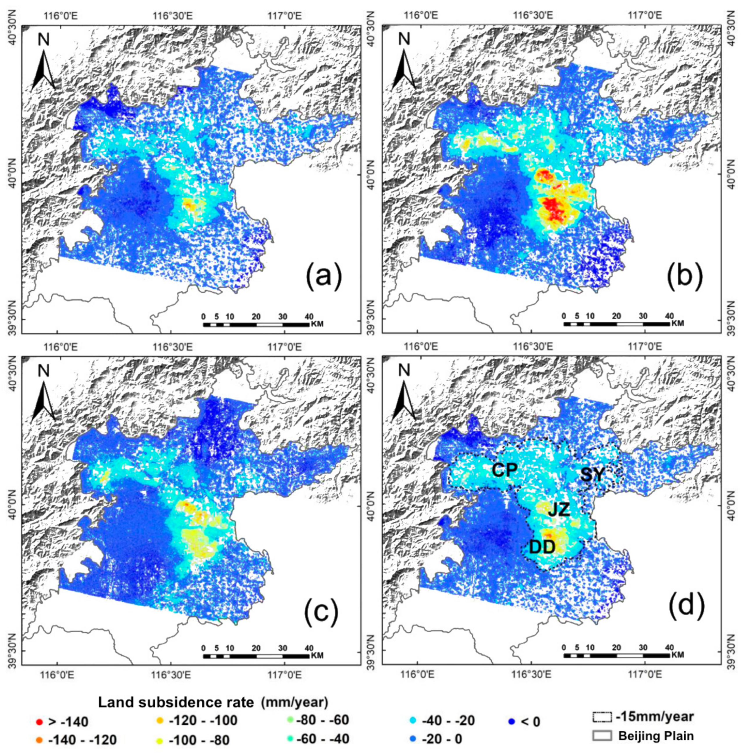
As shown in
Figure 7, the spatial distribution of land subsidence rates in the Beijing Plain is quite different and not uniform. Land subsidence centers are in Chaoyang and Tongzhou in the east, and Changping and Shunyi in the northeast and north of the Beijing Plain. The Dongbalizhuang–Dajiaoting subsidence center (DD) and the Chaoyang Jinzhan subsidence center (CJ) are notable for their extensive history of subsidence, whereas the Changping subsidence center (CP) and the Shunyi subsidence center (SY) have seen a more gradual emergence of subsidence phenomena in recent years. Analyzing subsidence rates across different intervals, the maximum annual average subsidence rates recorded were 137 mm/year for 2003–2010, 161 mm/year for the shorter interval of 2010–2016, and 135 mm/year for 2017–2020 (
Figure 7a–c). The apparent peak in subsidence rates during the 2010–2016 period must be interpreted with caution, given the shorter duration of this interval compared to the others. Notwithstanding, a notable trend of subsidence severity is observed during this time, with an indication of subsidence reduction from 2017 to 2020. Integrating these observations over the extended timeline from 2003 to 2020 through time series fusion reveals a long-term subsidence rate, with the highest annual average of 139 mm/year identified at the Dongbalizhuang–Dajiaoting subsidence center (DD) in the Chaoyang District (
Figure 7d).
3.2. Time Series Fusion of Land Subsidence from Envisat ASAR and Radarsat-2
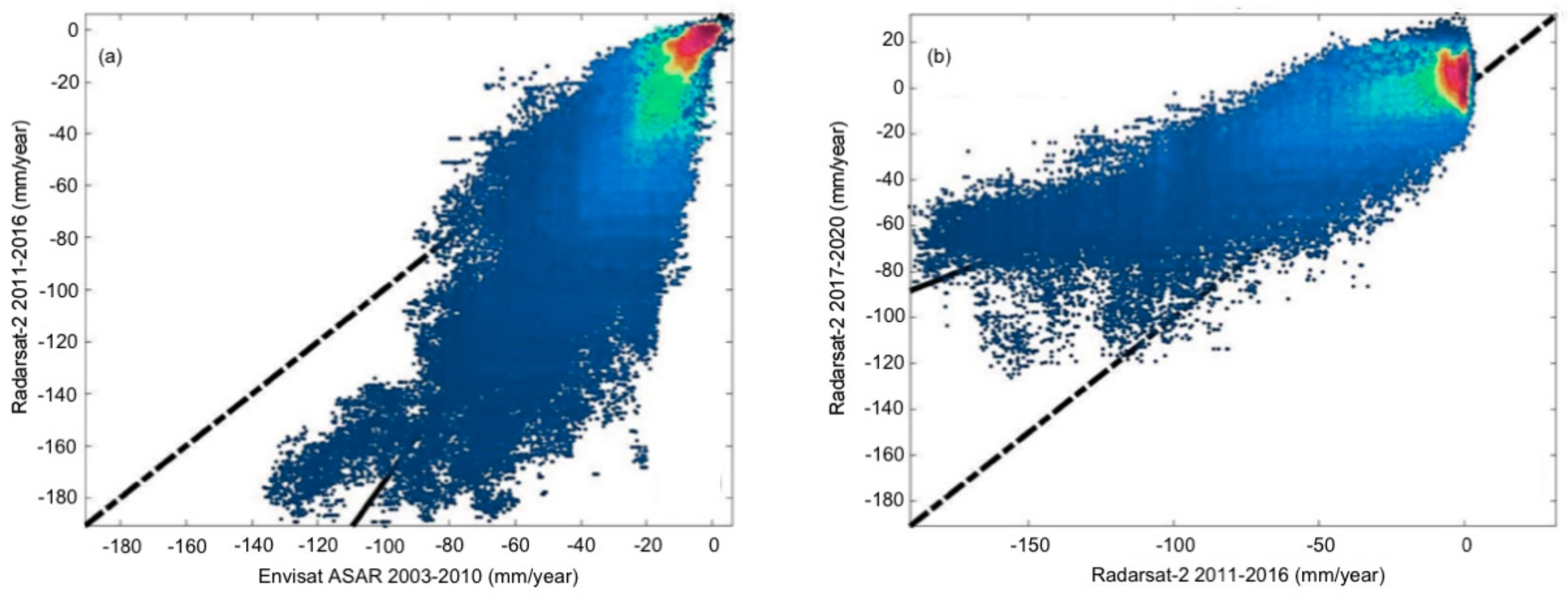
In this paper, 931,543 PS points were identified by a recent neighborhood method as eponymous sites for Envisat ASAR and Radarsat-2. The mean annual subsidence rates of InSAR monitoring in the Beijing Plain from 2003 to 2010, 2010 to 2016, and 2017 to 2020 were compared (
Figure 8). As shown in the graph, the average annual deformation rate over different time periods has a high correlation. Envisat ASAR and Radarsat-2 had an R
2 of 0.82, and Radarsat-2 (2011–2015) and Radarsat-2 (2017–2020) had an R
2 of 0.74, respectively. It is worth noting that compared to 2003–2010, about 92.2% of PS points settled in 2010–2016 (in
Figure 8a below x = y line), and about 86.1% of PS points settled in 2017–2020 compared to 2011–2016 (in
Figure 8b above x = y line). This indicates that the land subsidence increased significantly in 2010–2016 and decreased markedly in 2017–2020 during the three monitoring periods.
3.3. Land Subsidence Accuracy Verification
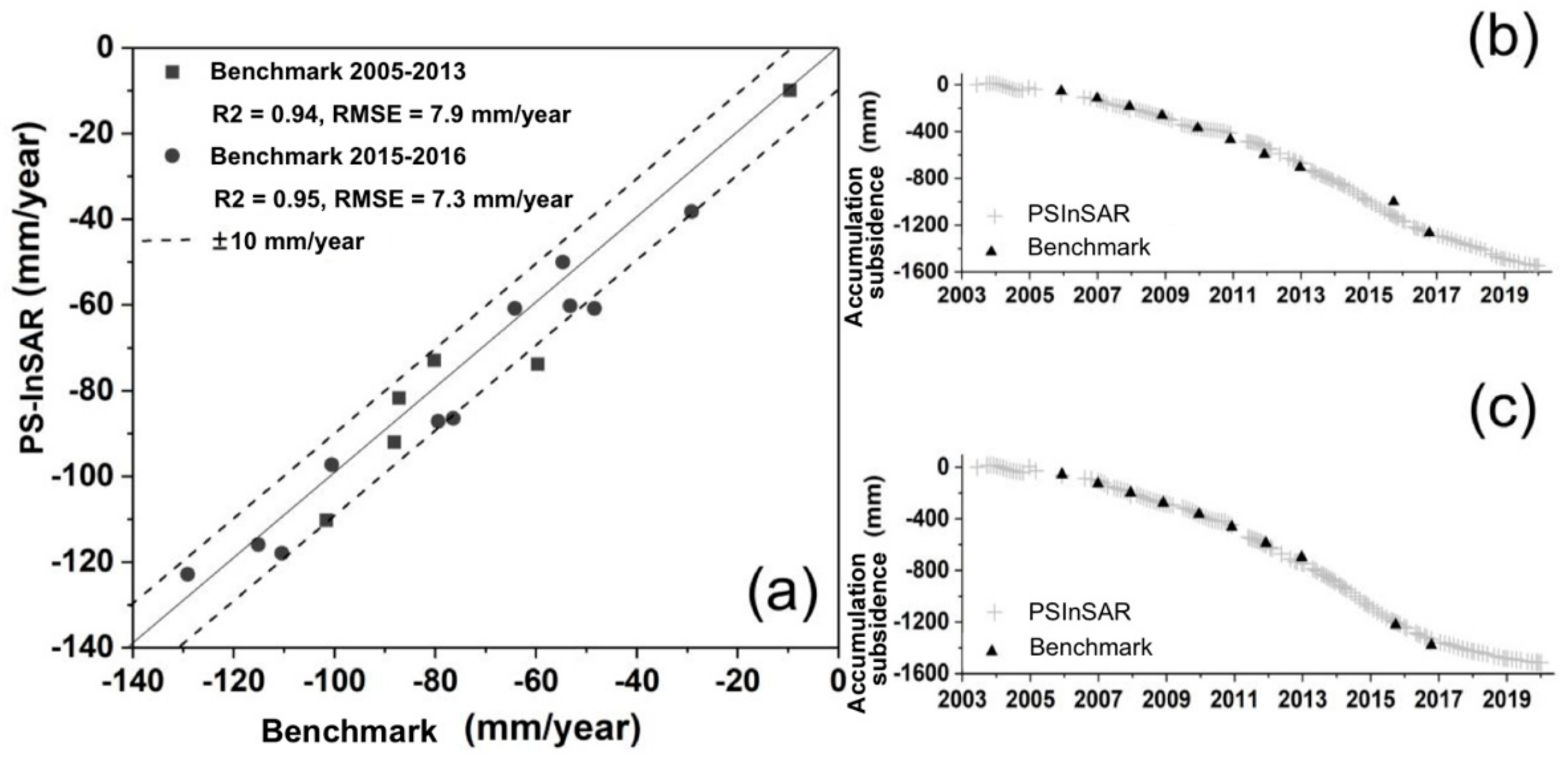
To validate the accuracy of PSInSAR and time series fusion processing results, we selected 6 leveling points from 2005 to 2013 and 11 leveling points from 2015 to 2016 to validate the accuracy of PSInSAR monitoring and time series fusion results. We compared the results of all PS points within 100 m of the level points with the mean values of all PS points within 100 m of the level points. The results showed a margin of error of 0.23 to 14.20 mm/year for both types of monitoring results for 2005–2013. In 2015–2016, the margin of error for both monitoring results was 0.89 to 12.39 mm/year. By correlation analysis, the linear regression correlation coefficients R
2 were 0.94 and 0.95, respectively, and the root mean square errors (RMSEs) were 7.9 mm/year and 7.3 mm/year, respectively (
Figure 9). The result of PSInSAR monitoring is more accurate and the accuracy meets the requirement. From the time trend, the amount of land subsidence obtained by the two monitoring methods had the same trend and indicated that the cumulative amount of land subsidence is increasing. However, the metamorphosis sequences monitored by PSInSAR have distinct nonlinear characteristics and more detailed information than those monitored at lower levels of the time spectrum (
Figure 9b,c). The difference between the two monitoring results is mainly due to temporal and spatial differences in monitoring data and errors in level monitoring and PSInSAR monitoring.
3.4. Wavelet Decomposition of Land Subsidence
In this study, we employed the Kriging interpolation method to estimate land subsidence values at unmeasured locations. Kriging is a geostatistical interpolation technique that takes into account the spatial correlation between measured data points to generate a continuous surface representation.
Figure 10 shows the interpolated map of land subsidence across the study area. The color gradient represents the magnitude of subsidence, with warmer colors indicating higher subsidence rates. The interpolated results provide a visual representation of the spatial patterns and variations in land subsidence, helping identify areas of interest. To evaluate the accuracy of the interpolation, a cross-validation analysis was performed. The mean error and root mean square error (RMSE) were calculated to assess the performance of the interpolation model [
44]. The results indicate that the interpolation method provides reasonably accurate estimates of land subsidence, with low mean errors and RMSE values.
The interpolated land subsidence data served as the input for the subsequent wavelet decomposition analysis, enabling a multi-level analysis of subsidence patterns at different scales. This integration allowed for a more detailed examination of localized subsidence features and their relationship with other factors of interest.
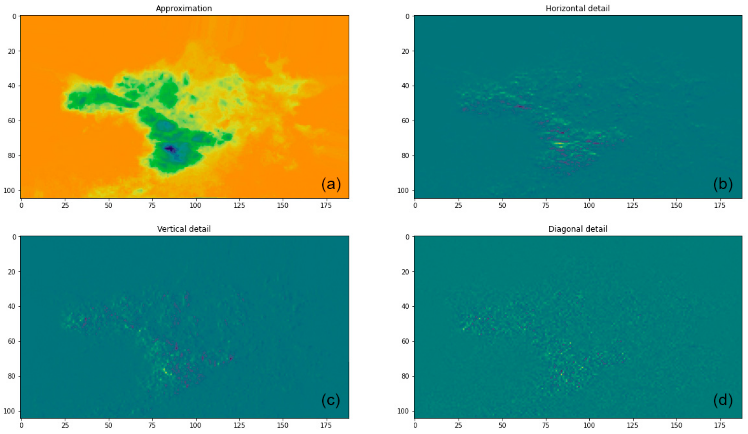
Wavelet decomposition was performed on the land subsidence data to analyze the variations and patterns at different scales. This technique allows for a detailed examination of localized features and provides valuable insights into the underlying dynamics of land subsidence. The land subsidence data were decomposed using the discrete wavelet transform (DWT) technique. The DWT breaks down the 2D signal into different frequency components, capturing variations at different scales.
Figure 11 illustrates the wavelet decomposition results, showing the subsidence coefficients. The decomposition coefficients represent the magnitude and spatial distribution of subsidence patterns. High-frequency coefficients correspond to localized subsidence features, while low-frequency coefficients capture broader-scale trends. The wavelet decomposition results were further integrated with other factors, such as building density, groundwater levels, and clay thickness. This integration helps identify potential correlations and interactions between land subsidence and these influencing factors.
3.5. Spatial Distribution of Groundwater, Compressible Clay, and Ground Building Density of Different Scales
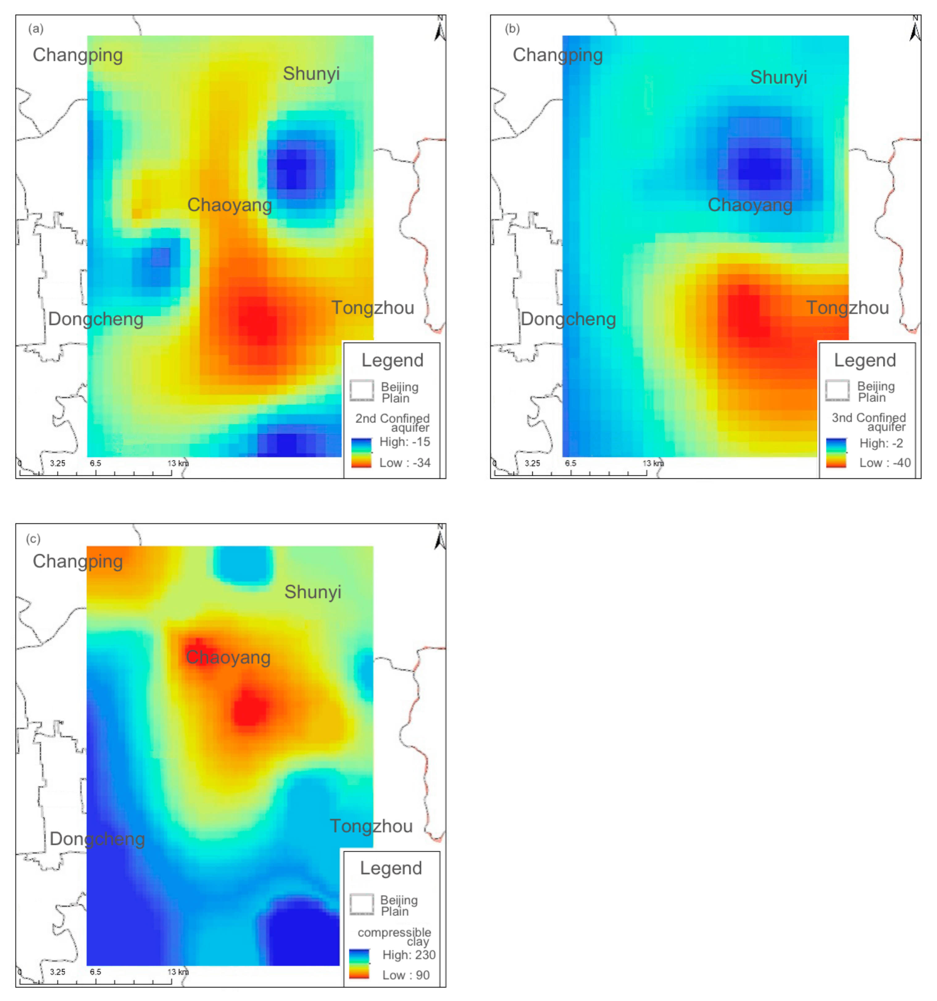
To analyze the spatial distribution characteristics of the main factors affecting land subsidence, the spatial autocorrelation of the main factors influencing the spatial stability of the second and third confined aquifers and the thickness of the compressible clay was adopted in this paper to reflect the spatial distribution characteristics of each element [
45].
As shown in
Figure 12a,b, both the second and third confined aquifers showed stable spatial variability within the study area, and Moran’s I values in both the second and third confined aquifers were greater than 0.9, showing a high spatial autocorrelation, indicating a more moderate spatial variability in the confined aquifers.
The spatial distribution of the compressible clay is shown in
Figure 12c. The spatial variation of the thickness of the clay was stable in the study area. The Moran’s I value of the thickness of the clay was 0.98 and showed a higher spatial autocorrelation, indicating that the thickness of the compressible clay also changed more smoothly in space.
Fishnet grids of 30 × 30 m
2, 60 × 60 m
2, 120 × 120 m
2, 240 × 240 m
2, 480 × 480 m
2, and 960 × 960 m
2 were generated to calculate the floor area within the grid and calculate the building density. The global Moran’s I index, which calculates building density at different granularities, decreased with increasing granularity, as shown in
Table 2, and fell below 0.1 when the cell size was 240 m and 960 m. It shows that the spatial autocorrelation of building density decreases gradually, and its distribution is more and more close to random distribution. The high-frequency part of the land subsidence and the low-frequency part are obtained by multistage wavelet decomposition. The low-frequency part of the land subsidence is a continuous change in space, showing a high degree of spatial autocorrelation. The Moran’s I value is close to 1, while the high-frequency part reflects the detailed features of the land subsidence, showing a degree of random distribution in space, showing a low degree of spatial autocorrelation, and the Moran’s I value is close to 0. Therefore, when the density of surface buildings is 240 m and 960 m, the spatial distribution characteristic is the same as that of the high-frequency part of the land subsidence. Therefore, in the analysis of the correlation between building density and land subsidence, the high-frequency distribution characteristics of the spatial random land subsidence and the building density were selected for the correlation analysis.
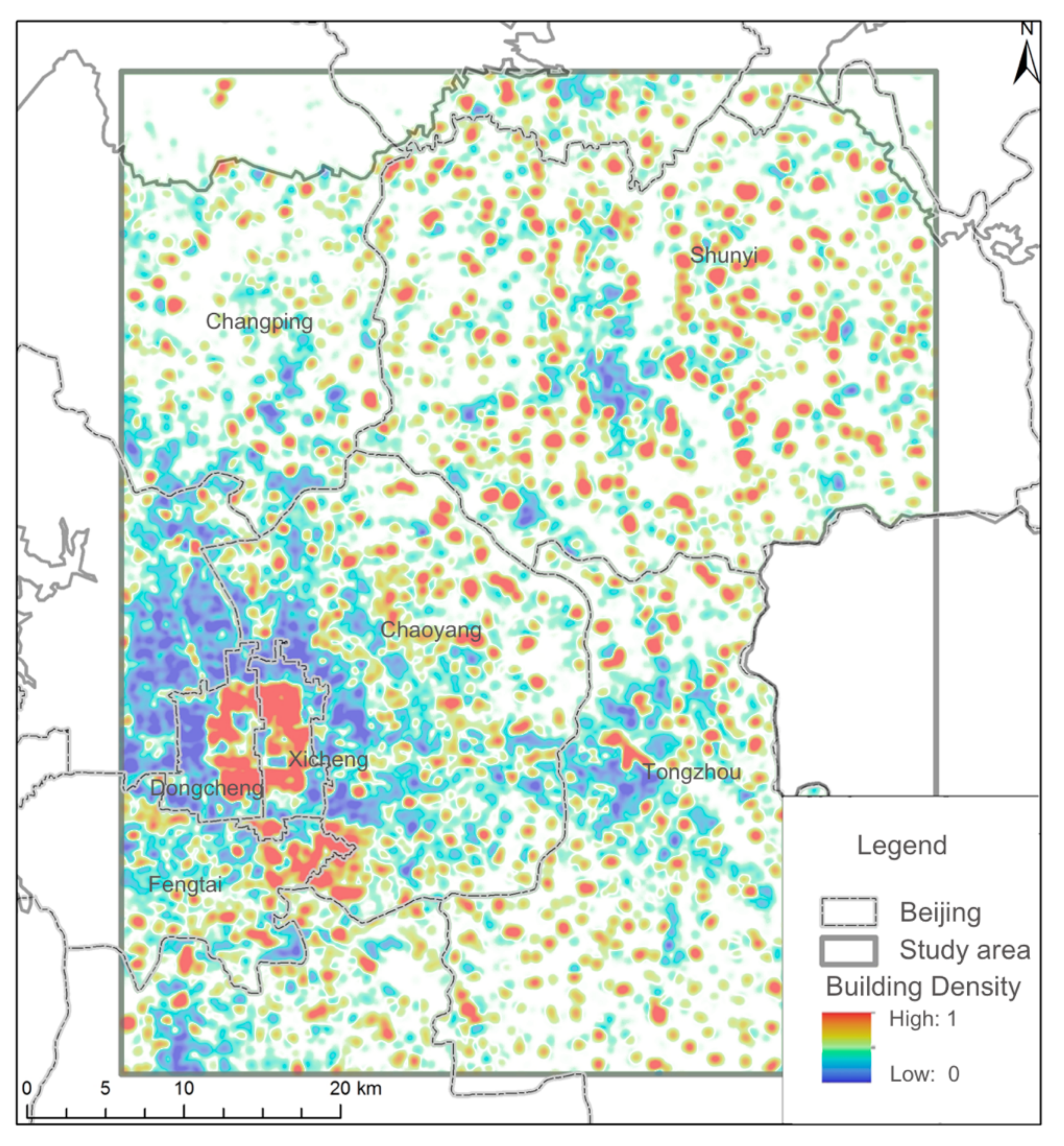
Figure 13 shows that the spatial distribution of building density did not show a clear global spatial cluster pattern, but there was a more significant clustering phenomenon in the small area, indicating that the spatial relationship between building density and factors in the small area is stronger and more likely to influence land subsidence.
3.6. Relationship between Ground Building Density and Land Subsidence at Different Scales
Because the building density is insensitive to the variation of the amplitude, the spatial distribution characteristic of the building density was selected as the calculation range of the regional amplitude and includes five settlement centers in the northern part of the Beijing Plain.
Generated fishnet grids of 30 × 30 m
2, 60 × 60 m
2, 120 × 120 m
2, 240 × 240 m
2, 480 × 480 m
2, and 960 × 960 m
2 were used to calculate the floor area within the grid and calculate the building density. The global Moran’s I index, which calculates building density at different granularities, decreases with increasing granularity, as shown in
Table 2, and falls below 0.1 when the granularity is 240 m and 960 m. It shows that the spatial autocorrelation of the building density decreases gradually, and its distribution is more and more close to random distribution. The high-frequency part of the land subsidence and the low-frequency part are obtained by multistage wavelet decomposition. The low-frequency part of the land subsidence is a continuous change in space, showing a high degree of spatial autocorrelation. The Moran’s I value is close to 1, while the high-frequency part reflects the detailed features of the land subsidence, showing a degree of random distribution in space, showing a low degree of spatial autocorrelation, and the Moran’s I value is close to 0. Therefore, when the density of surface buildings is 240 m and 960 m, the spatial distribution characteristic is the same as that of the high-frequency part of the land subsidence. Therefore, in the analysis of the correlation between building density and land subsidence, the high-frequency distribution characteristics of the spatial random land subsidence and the building density were selected for the correlation analysis.
Considering the local clustering of surface building density, the correlation between the high-frequency coefficient of land subsidence and building density was analyzed in the range of > 0.5 degrees of surface building density clustering, and the correlation coefficient was 0.29076 as shown in the table. With the increase in granularity, a more significant correlation occurred at the fourth stage of decomposition (
Table 3). It was shown that the density of buildings is more likely to influence the land subsidence at this scale.
The relationship between the main influencing factors and land subsidence is nonlinear. Previous studies have mainly selected typical research objects in small areas for analysis, and it has been revealed that there is a certain correlation between the surface building load and land subsidence in a particular area. In the area of the Beijing Plain, there is a significant correlation between the water level of the second confined aquifer and the thickness of the compressible clay and the land subsidence. In the analysis of the relationship between the surface building load and the land subsidence, the expression of the correlation is easily masked by the main influencing factors such as the thickness of the groundwater and the compressible clay layer.
As can be seen from the results of the spatial distribution of groundwater and compressible clay, Moran’s I values of the groundwater and compressible clay layers are both greater than 0.9 at different granularities, and the spatial distribution shows a significant spatial autocorrelation, with spatial distribution characteristics like those of low-frequency parts of the land subsidence rate wavelet decomposition. According to the spatial distribution of the factors influencing the quality of the area, the correlation between the water level of the second and third confined aquifers and the low-frequency part of the land subsidence was 0.77 and 0.74. The correlation between the thickness of the compressible clay and the land subsidence under different granularity was 0.71 and the fluctuation was not more than 0.01, indicating that the correlation between the thickness of the compressible clay and the high land subsidence was consistent with the results of previous studies in Beijing. According to the Moran’s I values of the thickness of groundwater and compressible clay and their high correlation with the low-frequency part of the land subsidence, the relation between the thickness of groundwater and compressible clay and the low-frequency part of the land subsidence is separated by wavelet decomposition.
Spatial Self-Correlation (SCOR), which shows the SCOR of buildings with low SCOR, is usually stochastic in nature, such as in residential neighborhoods and commercial street areas. The boundary size, combined with the SCOR of buildings with low SCOR, shows that the SCOR of buildings with low SCOR is not consistent with SCOR.
4. Discussion
According to the analysis of the distribution of the main factors influencing land subsidence, there is a strong correlation between key geological factors like groundwater and compressible clay layer thickness, and the low-frequency components of land subsidence. This relationship is further emphasized by the high spatial autocorrelation observed with these geological features.
The results of the study are supported by a robust spatial autocorrelation analysis which used Moran’s I to demonstrate a significant correlation between the geological factors and the low-frequency components of land subsidence. Specifically, both the second and third confined aquifers exhibited high spatial autocorrelation, as indicated by Moran’s I values greater than 0.9, suggesting a moderate spatial variability within these geological features. Similarly, the compressible clay layer showed a stable spatial variation, with a Moran’s I value of 0.98, indicating a smooth spatial change. This high degree of spatial autocorrelation in the geological factors aligns closely with the low-frequency components of land subsidence, highlighting their significant influence on the overall subsidence process. Furthermore, it was found that the relationship between the main influencing factors and land subsidence is nonlinear. The correlation between the water level of the second and third confined aquifers and the low-frequency component of land subsidence was notably strong, as was the correlation between the thickness of the compressible clay and land subsidence. These findings are consistent with previous studies conducted in Beijing, underscoring the importance of considering these geological factors in the analysis of land subsidence.
In explaining the relationship between surface building density and land subsidence at different scales, fishnet grids of varying sizes were utilized to calculate the building density. The results showed a gradual decrease in spatial autocorrelation with increasing granularity, indicating a shift towards a more random distribution. Notably, the high-frequency components of land subsidence, which were obtained through multistage wavelet decomposition, correlated well with the spatial randomness of building density, particularly at grid sizes of 240 m and 960 m. This suggests that in the context of building density and land subsidence, it is the high-frequency distribution characteristics that are more relevant for correlation analysis. These findings also revealed a unique trend at these scales. Particularly, at 480 m granularity, the Moran’s I value for building density was 0.02, indicating an almost random distribution of building density. Furthermore, the correlation coefficient between building density and the high-frequency component of land subsidence at this scale was 0.29076, which was the highest among all the granularities examined. This significant correlation persisted with little variation at the 960 m granularity, suggesting a consistent relationship between building density and land subsidence within the 480 m to 960 m granularity range. For Beijing, a granularity range of 480 m to 960 m typically encompasses the area of a residential community. This implies that within such neighborhoods, there is a notable correlation between building density and land subsidence.
While some studies suggest that building density does not significantly influence land subsidence, such as the research conducted by Yang and Ke [
46], our analysis presents a different perspective. Yang and Ke’s work, which concludes that land subsidence in Beijing is primarily governed by hydrogeological factors rather than urban construction aspects, contrasts with these findings. This research, which employed a multi-scale approach, revealed a nuanced correlation between building density and the high-frequency components of land subsidence at specific scales, particularly noticeable in the 480 m to 960 m granularity range. This distinction in these results highlights the complexity and scale-dependency of land subsidence, indicating that urban construction factors, including building density, can have varying impacts depending on the scale of analysis. Therefore, this study provides a new dimension in understanding land subsidence, emphasizing the significance of analyzing urban development impacts at different spatial scales.
However, this analysis also encountered several uncertainties. Firstly, due to the limited spatial scope of the data, wavelet decomposition was only feasible up to 960 m. An attempt to extend the decomposition to 1920 m resulted in insufficient data quantity, rendering the results of further analysis unreliable. Moreover, the trend of correlation between building density and land subsidence increased slightly from 30 m to 480 m and then showed a minimal decrease at 960 m. Due to the inability to analyze further decomposition stages, there is some uncertainty regarding the continuous trend of this correlation at extended stages. Additionally, it is crucial to acknowledge that land subsidence is a complex, nonlinear process influenced by multiple factors beyond just surface building construction. Therefore, while the current analysis provides significant insights into the correlation between building density and the high-frequency components of land subsidence, a more comprehensive investigation encompassing larger areas, such as the entire North China Plain, is required. This region is known for its pronounced subsidence issues, making it ideal for further study in this field of research. By extending this research to such a broader geographical scope, further analysis can be conducted to study the influencing factors in detail at even more granular levels, uncovering additional spatial characteristics. By conducting such an expanded analysis, it would further define or determine the correlation between land subsidence and surface building density, enhancing the understanding of the dynamics and scale of this complex phenomenon.
5. Conclusions
This study employed a multi-level two-dimensional wavelet decomposition to analyze land subsidence’s spatial characteristics at various scales while providing a nuanced understanding of its distribution across the study area. This method is instrumental as it can be used for the identification of specific areas affected by subsidence, facilitate informed decision making, and support mitigation efforts.
With the use of the global Moran’s I index analysis tool, spatial characteristics of potential contributors like building density, groundwater, and clay thickness were examined as they were integrated with land subsidence data, and key results were determined. This comprehensive approach can aid in formulating effective strategies for subsidence prevention and mitigation. The main findings include the following:
The utilization of two-dimensional wavelet decomposition offers localized insights into land subsidence across different scales. When coupled with Moran’s I statistical analysis, it provides a precise assessment of the discrete subsidence distribution in the study area. This method provides a detailed and comprehensive evaluation of local subsidence patterns.
Acknowledging the complexity of land subsidence, where influencing factors exhibit nonlinear effects, the study investigated the correlation between surface building density and land subsidence in the northern Beijing Plain at different granularities. This investigation revealed significant insights into the interactions between these factors.
An increasing correlation between building density and land subsidence was observed with rising granularity, particularly at 480 m and 960 m particle sizes. This discovery underscores the importance of granularity in understanding the dynamics between surface building density and land subsidence.
In conclusion, this study illustrates the intricate nature of land subsidence and the critical role of granularity in assessing the relationship between surface building density and land subsidence. These insights offer valuable guidance for policymakers, engineers, and researchers in developing strategies to mitigate the effects of land subsidence, ultimately protecting communities and the environment from its impacts.


