Conservation Planning of Multiple Ecosystem Services in the Yangtze River Basin by Quantifying Trade-Offs and Synergies

Abstract

The importance of protecting ecosystem services has been increasingly recognized due to their substantial benefits for human beings. Traditional conservation planning methods for locating and designing prioritized areas focus on high-value areas. However, ecosystem services have an intrinsic correlation of trade-offs and synergies among them; thus, solely selecting high-value areas cannot ensure efficiency in the conservation of multiple ecosystem services. Pursuing the protection of one ecosystem service may compromise the effectiveness of conserving others. Therefore, this study aims to develop a method for identifying the optimal ecosystem service protected areas in more efficient ways by quantifying the spatial relationships of ecosystem services on a local scale. We examined the correlations between all possible paired combinations of four ecosystem services using the Local Moran’s I and classified them into five cluster types in the Yangtze River Basin. To address conflicting solutions for multiple ecosystem service goals, we employed systematic conservation planning to identify priority areas for ecosystem service protection, following the principles of representativeness, complementarity, and persistence. By establishing scenarios that optimize each and all ecosystem services at target levels of 20%, 40%, 60%, and 80%, we observed that any two of the four services were positively correlated, occupying vast areas in the Yangtze River Basin. However, the high-value areas of each ecosystem service did not coincide in their spatial distributions. Under the same target, more high-value areas could be selected as the best solutions by only optimizing a single ecosystem service. The degree of overlap between priority areas varied considerably across optimizations for individual ecosystem services, particularly when setting lower targets. Our findings suggest that integrated conservation planning for all ecosystem services is more efficient than layering multiple single plans. Understanding the correlations between ecosystem services can lead to more effective management and sustainable decision making.

1. Introduction

Ecosystem services offer various direct or indirect positive benefits of nature to people, which are categorized by the Millennium Ecosystem Assessment (MEM) as provisioning, regulating, cultural, and supporting services [1]. Ecosystem services are increasingly being destroyed and threatened due to the utilitarian consumption of natural resources [2,3]. Biodiversity has long been the uppermost concern in conservation planning, and over the last decade or two [4,5,6,7], high-value ecosystem service areas have become of great importance [8,9,10]. Researchers have called for ecosystem services to be included in conservation planning [11,12,13,14]. The Kunming–Montreal Global Biodiversity Framework also reached an agreement stating that a target of no less than 30% of the world’s terrestrial, freshwater and marine areas, especially areas of significant value in relation to their biodiversity and ecosystem services should be maintained with effective conservation and management (22 December 2022, https://www.un.org/).

Conservation planning uses customized rules to identify optimal geographic areas of conservation features with significant natural resource value. The efficacy of conservation planning lies in achieving conservation goals under restricted conditions [15,16]. The fundamental mathematical theory of conservation planning is tackling the problem of maximal coverage or the minimal set problem, which is to cover all elements of conservation while keeping the cost as low as possible [17,18]. Several popular conservation planning theories have been put forward since the early 1880s [19,20]. One representative method is biogeographic regionalization, which divides the regions into similar or identical units by topography, hydrology, temperature, soil, etc. [21]. On the other hand, the hotspot method tries to protect the areas with high species richness, which raises the probability of species with maximal element cooccurrence being included [22]. With few exceptions, the commonality of these methods exclusively counts on their consideration of high-value areas, where the species are either high in amounts or exhibit high diversity. Though most valuable regions are included in the final planning, some rare or endemic species might be missed [23,24]. To compensate for these disadvantages, systematic conservation planning (SCP) carries out the planning with the principles of representativeness, complementarity, and persistence, providing a foundation to achieve conservation goals comprehensively and efficiently [15]. Widespread successful practices have been implemented using SCP to look for additional areas from existing reserves of networks or to design brand-new portfolios of protected areas.

Conserving ecosystem services is not fully the same as preserving biodiversity. Ecosystem services have two unique characteristics that are different from biodiversity. One is that the measured value for an ecosystem service is a continuous variable, while the estimated value for biodiversity is a discrete variable. Traditional biodiversity goals are a count of the number of species, while ecosystem service values can be subdivided. Ecosystem services lack movability and consecutive distributions compared to biodiversity. Another factor is that interactions with trade-offs and synergies exist among different ecosystem services [25,26,27]. Preserving one ecosystem service would be at the expense of disregarding the others [28]. Likewise, exploring the correlations between habitat quality (biodiversity) and other ecosystem services is one of the focus points of existing research [29,30,31], but opinions are divergent regarding their spatial congruence, and the correlations have been found to be both positive and negative [17,32,33]. Given this case, striving to find correlations rather than to quantify and optimize ecosystem services with SCP would be harsh or meaningless. One reason for this divergence is that most studies capture the relationships of ecosystem services with the total value of the entire study area [34,35]. Also, spatial heterogeneity is apparent in ecosystem services, and conclusions may vary with different scales. Explicit calculation of the spatial correlation among ecosystem services is an essential prerequisite for figuring out conservation plans that consider trade-offs and synergies.

In this paper, we focus our analysis within the Yangtze River Basin (YRB). Our overarching aim is to identify optimal areas for conserving the maximum benefits of multiple ecosystem services with the trade-offs and synergies being considered. We estimate four ecosystem service values (habitat quality, carbon storage, environmental purification, and hydrological regulation) in the YRB. We use the Local Moran’s I to explore the spatial correlations of any two of the four ecosystem service values and classify them into five kinds of clusters. We set scenarios optimizing each of the ecosystem services and all of them at different target levels from 20% to 80% with the guidance of SCP, respectively. Based on this analysis, we attempt to address the following three questions: (i) How many of the four ecosystem service values do the YRB possess and what is their spatial correlation? (ii) How are ecosystem service values distributed in the best selected areas for conservation? (iii) What are the trade-offs and synergies between only optimizing one ecosystem service and optimizing multiple ecosystem services?

2. Materials and Methods

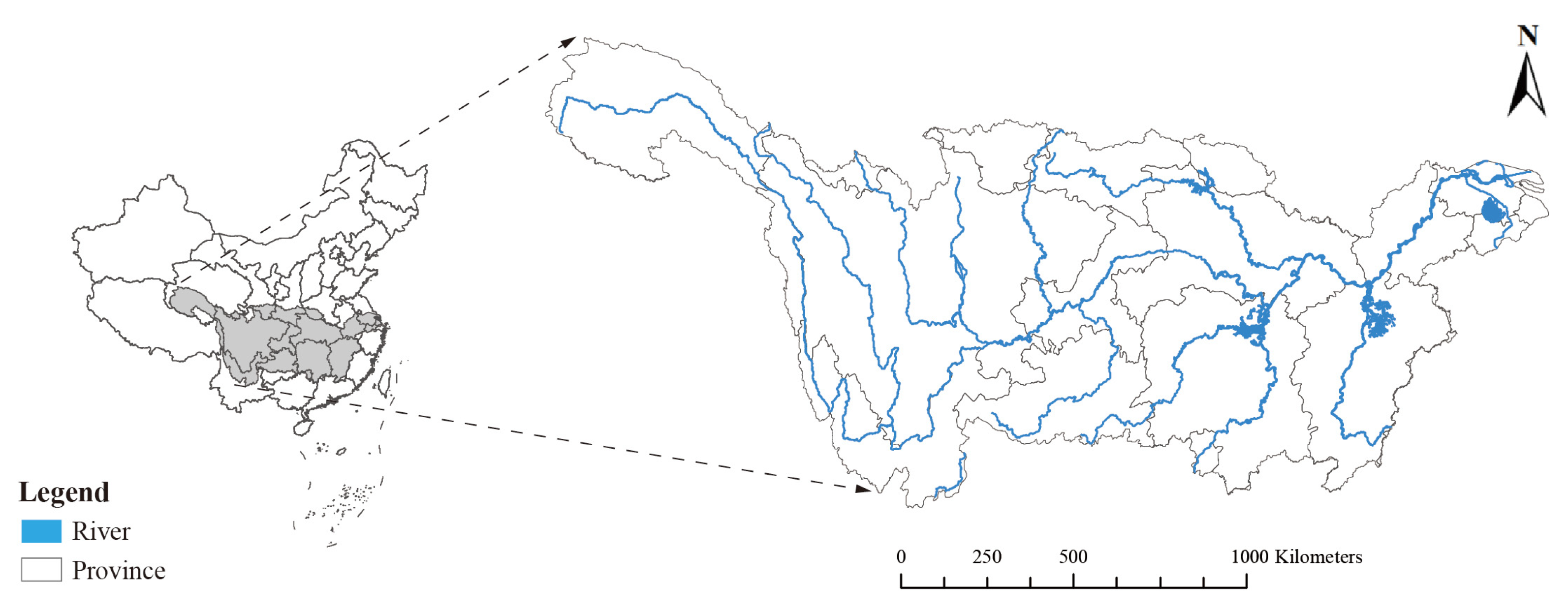
2.1. Study Area

The YRB (24°30′~35°45′ N, 90°33′~122°25′ E) (Figure 1) is an area of approximately 1.8 × 10⁶ km² that extends by the Yangtze River, which is the third longest river in the world, with a length of 6300 km. The Yangtze River originates from the Plateau of Tibet and flows into the East China Sea, traversing nineteen provinces and three economic zones. The YRB stretches across varied climates, landforms, and ecosystems, where the difference in elevation between the top and bottom is about 5 km. The average temperature is −4 °C in the upper YRB and 4~20 °C in other regions. The precipitation is primarily influenced by monsoons and the landform: the annual average is 400~800 mm, and it is uneven in both spatial and seasons. The YRB has more than 7000 tributaries, contributing 35% of the total water resources in China, which is much higher than other basins.

2.2. Data Sources

This study evaluated the ecosystem service values of habitat quality, carbon storage, environmental purification, and hydrological regulation. The habitat quality was estimated with the Maxent model, the species distribution data were downloaded from IUCN (International Union for Conservation of Nature, https://www.iucn.org) and GBIF (Global Biodiversity Information Facility, https://www.gbif.org), and the weather and climate data were from WorldClim (https://www.worldclim.org), with a spatial resolution of 30 seconds. The carbon storage was calculated with the inversion equation, in which the NDVI was downloaded from the GIMMS Global Agricultural Monitoring website (https://glam1.gsfc.nasa.gov), and the vegetation data was from the geographic data platform of Peking University (https://geodata.pku.edu.cn). Environmental purification and hydrological regulation were estimated using the land-use/land-cover data obtained from the RESDC (Resources and Environment Science and Data Center, https://www.resdc.cn) with 1 km resolution in 2020, and the NPP (Net Primary Production) and precipitation data were obtained from the Geospatial Data Cloud (https://www.gscloud.cn/). The subcatchment data were from the BasinATLAS (http://www.hydrosheds.org) and served as planning units.

2.3. Estimation of Ecosystem Service Values

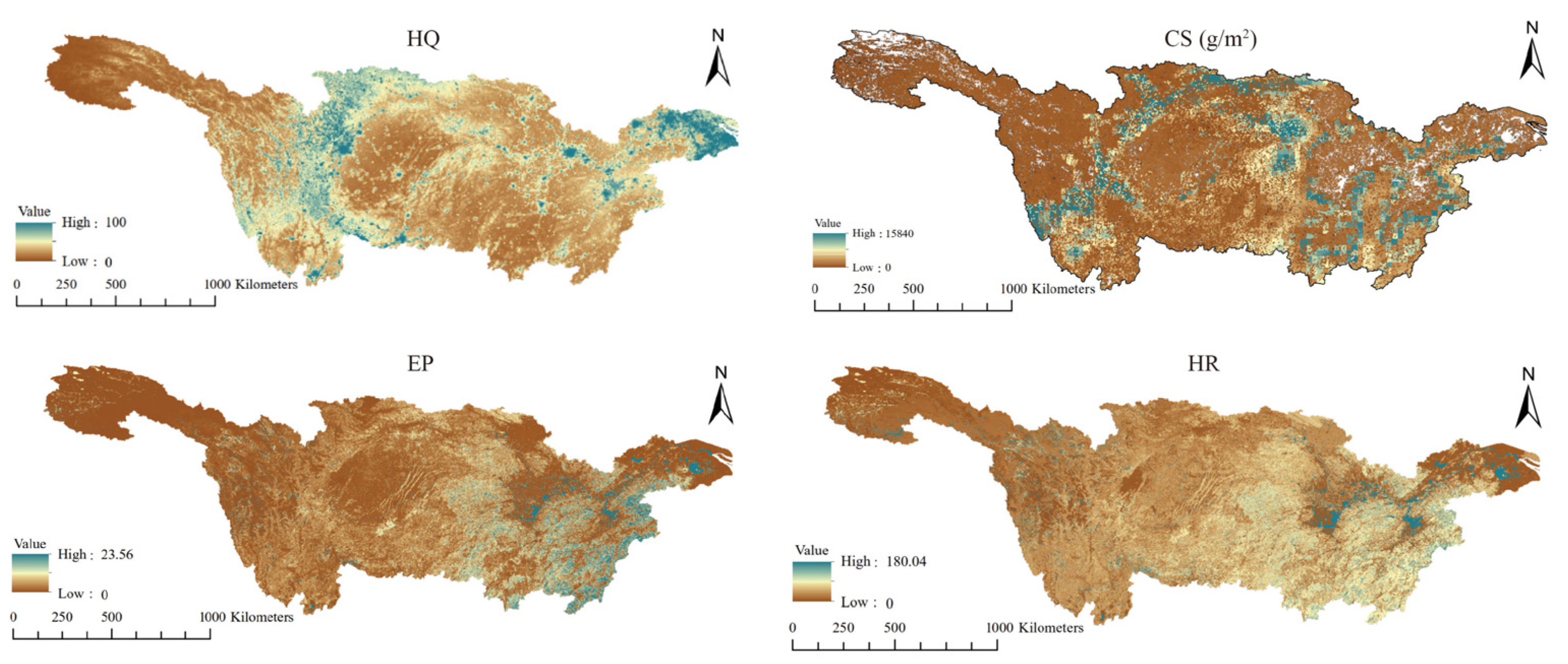
2.3.1. Habitat Quality

The habitat quality was assessed with the Maxent (version 3.4.3) software, which uses the maximum entropy algorithm to rate the species’ niches. The results were species occurrence probabilities, computed via a function composed of environmental factors. Threatened species are generally employed as a surrogate for biodiversity in data-scarce areas [36,37], and we thus chose the list of threatened species from the IUCN red list in China, which includes mammals, amphibians, and freshwater groups. The localities for each species were from GBIF. To raise the generalization performance of Maxent, we dropped the species that occurred lower than 30 times in the GBIF data. We selected 20 environmental factors to model the species’ niches: 19 were from WorldClim (details on these factors can be seen on the WorldClim website), and 1 was land use/land cover.

2.3.2. Carbon Storage

In this study, the carbon storage values were for vegetation, and consisted of the aboveground and belowground carbon storage. The aboveground carbon storage was calculated with an inversion function related to the NDVI and the biomass [38]. The belowground biomass was calculated using the belowground-to-aboveground biomass ratio regarding vegetation types [39]. This was also true for converting the biomass values to carbon storage values with a conversion factor (0.45). We classified the vegetation into forest, shrub, grassland, cropland, and marsh in our study.

2.3.3. Environmental Purification and Hydrological Regulation

We used an improved equivalence factor method to estimate the ecosystem service values of environmental purification and hydrological regulation, as followed by Xie [40]. Environmental purification refers to the removal and degradation of excessive nutrients and compounds by vegetation and organisms, as well as the retention of dust and pollution. This method first evaluates the value equivalence factor per hectare for 14 different types of terrestrial ecosystems, then uses a dynamic spatiotemporal modifier to reflect variations in each kind of ecosystem; the formulas were as follows:

$$F_{ij}=M_{ij}\times F_n$$

(1)

$$M_{ij}=\frac{B_{ij}}{\overline{B}}$$

(2)

where F_ij is the equivalence value of environmental purification/hydrological regulation in month j of area i; F_n is the equivalence factor of ecosystem service types; B_ij is the NPP/precipitation in month j of area i; and B is the annual average value of NPP/precipitation. NPP is the modifier of environmental purification, and precipitation is the modifier of the hydrological regulation; the ecosystem service equivalent value per unit area is based on the work of Xie [40].

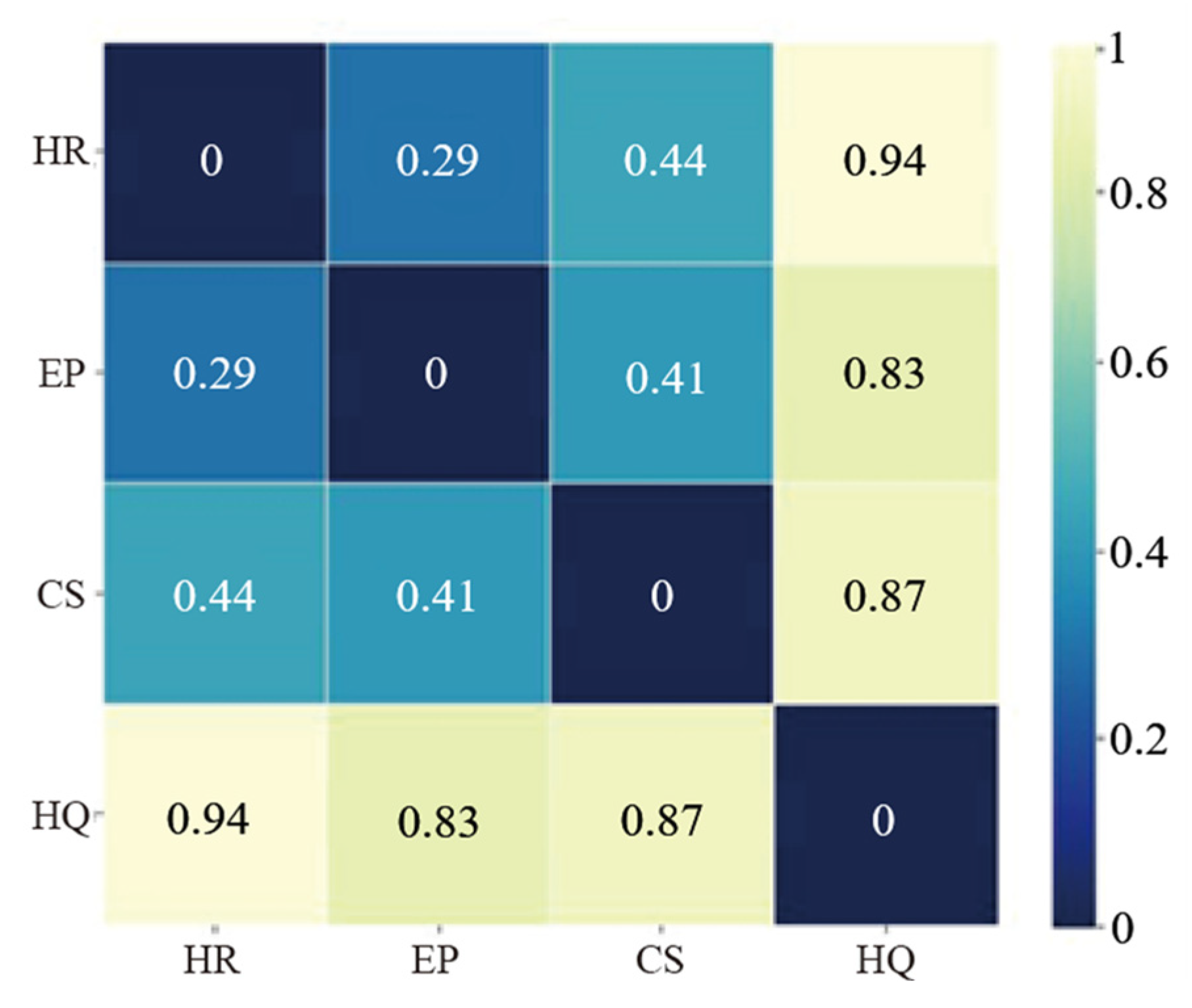
2.3.4. Analysis of Relationships among Ecosystem Services

The Local Moran’s I was applied to determine the trade-offs and synergies of the paired ecosystem services out of 4, which classifies them into 5 clusters according to their similarity: these are high-high (H-H), low-high (L-H), low-low (L-L), high-low (H-L), and not significant (NS). The formula was as follows:

$$\mathrm{I}=\frac{\left({\mathrm{x}}_{\mathrm{i}}-\overline{\mathrm{x}}\right)\sum _{\mathrm{j}=1}^{\mathrm{n}}{\mathrm{W}}_{\mathrm{ij}}\left({\mathrm{x}}_{\mathrm{j}}-\overline{\mathrm{x}}\right)}{\sum _{\mathrm{i}=1}^{\mathrm{n}}\left({\mathrm{x}}_{\mathrm{i}}-\overline{\mathrm{x}}\right)}$$

(3)

where I is the Local Moran’s I, whose value ranges from −1 to +1, where −1 indicates they are negatively correlated, +1 indicates they are positively correlated, and 0 indicates they are unrelated; W_ij is a weight matrix that represents the spatial configuration of the unit value of the raster data; i and j represent the types of ecosystem services; x is the ecosystem service value of the cell; and $\overline{x}$ is the average value of all units. The Local Moran’s I was computed in GEODA (version 1.16).

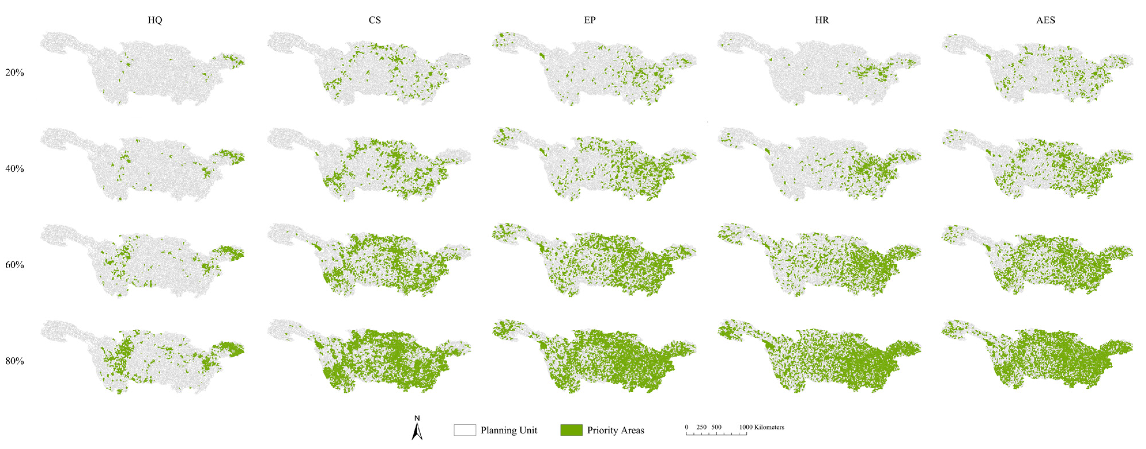
2.4. Spatial Optimization

We used MARXAN (version 1.8.2) to find the best areas for conserving ecosystem services, which is a software for designing protected areas based on the rules of SCP [41] (Ball, 2009). In this study, we divided the YRB into 6828 subcatchments (the average area was 246.21 km²) to serve as planning units, each with attributes of the conservation features (ecosystem service values) and the costs to be protected. Computationally, this method applies the “0–1” integer programming model to fit the problem,

$$Obj=\sum _i^{N_s}{x}_i{c}_i+b\sum _i^{N_s}\sum _h^{N_s}{x}_i\left(1-x_h\right)c{v}_{ih}$$

(4)

$$s.t.\hspace{1em}\sum _i^{N_f}{x_{i}r}_{ij}\ge T_j$$

(5)

where x_i is the planning unit i; in the result, i is either 0 for unselected or 1 for selected; c_i is the cost of the planning unit i; b is the boundary length modifier, which is used to modify the compactness of the selected planning unit, where the higher the value, the larger the clump size of the solution; cv_ih is the length of the shared boundary of planning unit i and h; r_ij is the value of feature j in planning i; and T_j is the target for feature j. In our study, we set targets to conserve 20% to 80% of each and all ecosystem services. MARXAN runs with the simulated annealing algorithm to solve the equations.

2.5. Measurement of the Similarity between Optimal Spatial Patterns

Jensen–Shannon divergence (JSD) was employed to measure the similarity of the two sets of planning units that were selected. Each planning unit was assigned a value in the form of a probability, which equaled the maximum value of all of the planning units divided by the ecosystem value of the planning unit being considered. We ran MARXAN 1000 times and generated an array of probability distributions; thus, the similarity of the distributions could be measured with JSD. The formula was as follows:

$$KL\left[P\left(X\right)\left|\right|Q\left(X\right)\right]=\sum _{x\in X}\left[P\left(x\right)\mathit{log}\frac{P\left(x\right)}{Q\left(x\right)}\right]$$

(6)

$$JSD\left(P\left(X\right)\right|\left|Q\right(X\left)\right)=\frac{1}{2}KL\left(P\left(x\right)\left|\right|\frac{P\left(x\right)+Q\left(x\right)}{2}\right)+\frac{1}{2}KL\left(Q\left(x\right)\left|\right|\frac{P\left(x\right)+Q\left(x\right)}{2}\right)$$

(7)

where P(X) and Q(X) are the probability distribution of optimizing each target. The JSD values range from 0 to 1, where 0 means that the two distributions are identical and 1 means that the two distributions are totally different.

2.6. Statistical Analysis of Ecosystem Service Value Distribution

We used the Natural Breaks algorithm to classify each of the four ecosystem service values into 7 levels (from the lowest, 1, to the highest, 7) and group similar values together to make each group have the maximum difference. To illustrate the distributions of high-value areas with or without systematic conservation planning, we counted the number of planning units at the classified levels and recorded them as a percentage of all planning units under all of the optimization scenarios. For instance, at the target of 20%, we made a statistical analysis of high-value areas for habitat quality by only optimizing habitat quality and all of the ecosystem services.

3. Results

3.1. Distribution and Trade-Offs of Ecosystem Service Supply Areas

The distribution of the habitat quality was clustered in plenty of lakes and river regions. The high-value areas of habitat quality were around the three biggest lakes along the Yangtze River (Figure 2), which are Dongting Lake, Poyang Lake, and Tai Lake. In addition, there were also areas eminently suitable for species to survive scattered downstream of the Jinsha River. The forest, shrubland, and grassland areas were the most critical contributors to carbon storage. Therefore, the carbon storage showed a situation where the northeast was high and the southwest was low; the carbon storage distribution also coincided with the Yangtze River Economic Belt, where urbanization encroaches on the natural forests and grasslands. The spatial characteristics of environmental purification were roughly opposite to those of the carbon storage, showing that the mid-west was low and the east was high. Similarly, environmental purification was very low in the Yangtze River delta, which has a high intensity of human interference and development. Hydrological regulation values were directly related to the water resources, being distributed in the regions of rivers and lakes.

The overall performance of the Local Moran’s I map (Figure 3) showed a positive correlation between four ecosystem services occupying large areas in the YRB. Large regions of H-H agglomeration exclusively existed between the HQ and CS in the junction regions between the upstream and midstream areas of the YRB. H-H agglomeration areas of EP and HQ, and HR and HQ were mainly distributed in the lower reaches of the YRB. The synergies of H-L agglomeration were significant for all ecosystem services in the midstream of the YRB. EP and HQ, and HP and CS, presented a homologous distribution of L-L agglomeration, and this was also true for EP and CS, and for HR and CS. Prominent areas of L-H agglomeration could be observed in the upper-middle reaches and delta of the YRB.

3.2. Priority Areas for Ecosystem Service Conservation

Setting targets for conserving each ecosystem service, the priority areas varied and were not the same under different target levels, which was particularly prominent at the target of 20%. As the target level increased, priority areas of CS, EP, and HR coincided. In contrast, nearly half of the HQ priority areas were not correlated with the other three ecosystem services, even if all of the planning units were selected (Figure 4). Only EP and HR showed a similar trend in the optimal spatial conservation pattern; these areas were concentrated in the east and at the source of the YRB (Figure 5). When conserving all of the ecosystem services, the priority areas were not merely an overlap of the results of optimizing each of the four ecosystem services; trade-offs were obvious between optimizing HR and optimizing all ecosystem services; and the JSD was 0.29, 0.44, 0.94 in order with EP, CS, and HQ (Figure 4). MARXAN tried to find the best solutions under the principles of representativeness and complementarity, and areas with high values of all of the target features have higher priority, so high-value areas with a single feature were not necessarily included. Another reason for this was that the HQ was distributed unevenly, so a small number of areas possessed much of the total amount. The same was true for CS, and the distribution for EP and HR was relatively uniform. Hence, their priority areas differed under a low target level but became more similar as the target level increased (Figure 4 and Figure 5).

To clarify the value composition under different optimization objectives, we further calculated the percentage of values for ecosystem services in accordance with maps of their spatial distribution (Figure 6). This clearly showed that more planning units at a high level (≥4) were selected as a higher priority in optimizing a single ecosystem service without the trade-off consideration among all of the ecosystem services. This was prominent when the target was low. For example, to conserve 20% of the habitat quality in the YRB, 90% of planning units at level 7 and 74% at level 6 were the best choices when optimizing habitat quality. In comparison, 63% of planning units at level 7 and 37% at level 6 were selected when optimizing all ecosystem services.

4. Discussion

Our study proposed employing the SCP theory to optimize the conservation of ecosystem services in an efficient way with the consideration of their trade-offs and synergies. We quantitatively evaluated the distribution of the HQ, CS, RP, and HR in the YRB. The measurement of JSD between each ecosystem service allowed us to find discrepancies in the optimal conservation solutions. A statistical analysis of the data’s distributions explained the efficiency of different conservation strategies. Undoubtedly, conservation planning under different target settings will produce multiple optimal spatial configurations with more or less differences. Drawing up plans that aim at only one objective and overlaying the results together will be of low efficiency with much more cost in terms of time and money. We thus introduced the principles of representativeness and complementarity, developing an approach of optimizing multiple ecosystem services comprehensively to balance the trade-offs among these conservation features based on multiple scenarios, which could provide preferential focal areas for their co-benefits and improve regional sustainability for managers to develop strategies of conservation.

Numerous studies have been conducted on the trade-offs and synergies of ecosystem services. However, they are predominantly interested in the relationship of the total amount of each ecosystem service, the driving factors, dynamic spatial and temporal changes in ecosystem services, and investigating higher-priority areas to be protected; the distributions of the selected areas are scarcely discussed [42,43,44,45]. To raise the accuracy of the trade-off analysis, we used MaxEnt to evaluate the suitability of biodiversity, and the NDVI, NPP, and precipitation as an adjustment layer to reflect the heterogeneity of the same land-use/land-cover type, which is a crucial factor in determining ecosystem services themselves. Similarly, ecosystem service value estimation models such as InVEST and CASA employ topographical, metrological, or soil-type data as correction factors. Even though this evaluation can be limited by the accessibility, scale, and time-sequential nature of the data, the values of the same land-use/land-cover type over different years are commonly homologous, which means that as long as the land is not transformed, the ecosystem service values would not be changed [46,47]. In addition, we used the Local Moran’s I to seek the relationship among ecosystem services, which is widely used in the field of economics [48]. Areas adjacent to the target areas also contributed to the calculation, which allowed us to explore the relationships of ecosystem services more accurately on a local scale. The spatial autocorrelation of the paired target areas was captured as clusters, and they were classified into five kinds. Ignoring the spatial proximity when calculating the correlations between ecosystem service values would mean each calculated area shares its maximum or minimum values with another certain region, leading to underestimation or overestimation of its trade-offs and synergies.

MARXAN, as a decision support tool, is mainly and extensively used in creating protected area systems aimed at conserving biodiversity or biodiversity surrogates [41], including character or trait diversity, species diversity, species assemblage, landscape pattern, and habitat diversity. SCP has been proven to be the best practice in biodiversity conservation. A few studies have tried to use MARXAN to make ecosystem service conservation planning; nonetheless, they either broke the study area into zones to develop corresponding management strategies [49] or simply aimed to maximize the benefits of protecting ecosystem services in their planning [50]. These all failed to consider the complementarity and spatial correlations of different ecosystem services in systematic conservation planning. Commonly, areas with the highest ecosystem service values should be selected. A typical and well-known area selection method that follows this concept is the hotspot method. Hotspots focus on choosing richness or range-size rarity in the species of the areas. Case studies show that the method of making rules from the perspective of conserving the biologically rich spots instead of the whole species will lead to some species being excluded from all of the species of the region in the final solution when the target level is not high, and more areas and economic cost would thus be needed.

Further, our statistical analysis of the ecosystem service value distribution showed that comprehensive planning for all of the ecosystem services was more efficient than optimizing each one alone. When the target level for conservation was raised, though the percentages of planning units to be included for both optimizing one ecosystem service alone or all ecosystem services were also increased, the planning units at a high-value level were not the best choices in the scenario of optimizing for all of the ecosystem services. When conserving 20% of all ecosystem services, the percentage of planning units at value levels 6 and 7 was obviously lower than that of the planning unit when optimizing HQ, CS, and HR alone. This implicated that there were trade-offs among the HQ, CS, and HR in their high-value areas. The Local Moran’s I cluster maps of the three paired ecosystem services also showed that H-H agglomerations were consistent in their value distributions, and these were in the lower reaches of the YRB. For EP, there was not much difference in the percentage of the planning units between optimizing just the EP and optimizing all of the ecosystem services. This indicated that the distributions of high-value areas for EP and the three other ecosystem services were synergetic. Hence, aiming at a single objective merely counting on the high-value areas was more efficient than considering the co-benefit areas with other ecosystem services [51], as it achieved the goal with less areas. It was obvious that when only concentrating on a single ecosystem service in low target levels, solitary high-value areas were selected merely because they had high values, thus achieving the goal faster regardless of their contribution to the whole region and enabling subsequent sustainable management.

In addition, it should be noted that there is complementarity among ecosystem services when developing optimal strategies to enhance them. The correlation matrix between ecosystem services can be viewed as their complementarity: the higher its value, the higher the complementarity between the two ecosystem services. This indicates that more areas would be needed to conserve both of the two ecosystem services. Moreover, areas with high complementarity will not necessarily be the high-value ones. For example, the JSD of HR and EP was 0.29, and the percentage values were nearly the same when optimizing each, but this differed when optimizing all of the ecosystem services. More areas at low-value levels were increasingly needed for achieving the goals. It is indisputable that if we concentrate on these seemingly valuable areas with single-objective planning, more resources would be consumed in the face of the new requirements. The selection of priority areas for all of the objectives should be handled systematically. The Chinese government has been promoting a “multi-planning integration” reform since 2014 (https://www.mnr.gov.cn), the core notion of which is to include multiple planning considerations in a single plan, such as considering national economy and social development planning, town and country planning, land planning, etc., to ensure that all of the planning can maintain inherent consistency across areas. Our methodology of analyzing the trade-offs and synergies of multiple ecosystem services could be used to investigate the cohesion mechanism of multi-planning. The advantages and disadvantages of different plans could be compared by means of the statistical analysis of ecosystem service value distribution. Lastly, our integrated conservation planning method for all ecosystem services is helpful in providing enlightenment for drawing up multiple plans on the same map to reconcile their benefits and conflicts.

Our study still has some limitations. Although we compared the trade-offs and synergies among ecosystem services, other correlations were not analyzed, such as the demand and flow [52,53,54]. The beneficiaries of ecosystem services are people and nature, and efficiency will go a step further if the flow paths between the demand areas and supply areas are identified, causing extra losses and costs in long-distance transmission [55]. Moreover, we did not incorporate restoration planning; ecological restoration projects could restore high-value ecosystem service areas, and the Chinese government are also implementing policies of ecological protection and restoration for mountains/rivers/forests/farmlands/lakes/grasslands. From the view of this prospect, our study proposed that governments, stakeholders, and managers should be involved together to develop strategies of conservation and restoration, and the trade-offs involved in meeting their goals are crucial in systematic planning. A comprehensive planning approach is more sustainable than piecing together multiple separate plans.

5. Conclusions

In this study, we aimed to develop an approach of identifying the priority areas for ecosystem service conservation to resolve the conflicts of trade-offs and synergies among different ecosystem services. To achieve this, we evaluated ecosystem service values of HQ, CS, EP, and HR in the Yangtze River Basin and analyzed their spatial correlations with five types of clusters on a local scale with the Local Moran’s I. Then, we set multiple scenarios for optimizing each ecosystem service alone and optimizing all of the ecosystem services together. Through statistical analysis and comparison of the spatial configurations after optimization, our results highlighted that an integrated systematic conservation planning involving all of the ecosystem services together is more efficient, as it uses less areas to provide an equal return of benefits, than superimposing multiple plans of optimizing one ecosystem service at a time. There are trade-offs and synergies among this optimization planning apart from the ecosystem services themselves as well. Taking complementarity into account in the planning made it not necessary to solely focus on the high-value areas. Concentrating on these seemingly valuable areas within single-objective planning will consume more resources in the face of the new requirements. This study also highlights some topics to be explored in further work, as some interactions between ecosystem services, such as their demand and flow, were ignored, and we also overlooked the impact that restoration planning could have on conservation planning. Despite this, our approach can aid planners to promote their planning by balancing the targets, costs, and benefits more efficiently.

References

1. Millennium Ecosystem Assessment (MEA). Ecosystems and Human Well-Being; Report of the Conceptual Framework Working Group of the Millennium Ecosystem Assessment; Island Press: Washington, DC, USA, 2003; p. 235. [Google Scholar]
2. Steffen, W.; Richardson, K.; Rockström, J.; Cornell, S.E.; Fetzer, I.; Bennett, E.M. Planetary boundaries: Guiding human development on a changing planet. Science 2015, 347, 1259855. [Google Scholar] [CrossRef] [PubMed]
3. Sutton, P.C.; Anderson, S.J.; Costanza, R.; Kubiszewski, I. The ecological economics of land degradation: Impacts on ecosystem service values. Ecol. Econ. 2016, 129, 182–192. [Google Scholar] [CrossRef]
4. Dudley, N. Guidelines for Applying Protected Area Management Categories; IUCN: Gland, Switzerland, 2008. [Google Scholar]
5. Goldman, R.L.; Tallis, H. A critical analysis of ecosystem services as a tool in conservation projects: The possible perils, the promises, and the partnerships. Ann. N. Y. Acad. Sci. 2009, 1162, 63–78. [Google Scholar] [CrossRef] [PubMed]
6. Boulton, A.J.; Ekebom, J.; Gislason, G.M. Integrating ecosystem services into conservation strategies for freshwater and marine habitats: A review. Aquat. Conserv. 2016, 26, 963–985. [Google Scholar] [CrossRef]
7. Hermoso, V.; Carvalho, S.B.; Giakoumi, S.; Goldsborough, D.; Katsanevakis, S.; Leontiou, S. The EU Biodiversity Strategy for 2030: Opportunities and challenges on the path towards biodiversity recovery. Environ. Sci. Policy 2022, 127, 263–271. [Google Scholar] [CrossRef]
8. McCann, K.S. The diversity–stability debate. Nature 2000, 405, 228–233. [Google Scholar] [CrossRef]
9. Balvanera, P.; Daily, G.C.; Ehrlich, P.R.; Ricketts, T.H.; Bailey, S.A.; Kark, S. Conserving biodiversity and ecosystem services. Science 2001, 291, 2047. [Google Scholar] [CrossRef]
10. Chan, K.M.A.; Shaw, M.R.; Cameron, D.R.; Underwood, E.C.; Daily, G.C. Conservation planning for ecosystem services. PLoS Biol. 2006, 4, e379. [Google Scholar] [CrossRef]
11. Egoh, B.; Rouget, M.; Reyers, B.; Knight, A.T.; Cowling, R.M.; Van Jaarsveld, A.S.; Welz, A. Integrating ecosystem services into conservation assessments: A review. Ecol. Econ. 2007, 63, 714–721. [Google Scholar] [CrossRef]
12. Reyers, B.; Polasky, S.; Tallis, H.; Mooney, H.A.; Larigauderie, A. Finding common ground for biodiversity and ecosystem services. BioScience 2012, 62, 503–507. [Google Scholar]
13. Ros-Cuéllar, J.; Porter-Bolland, l.; Bonilla-Moheno, M. Can Multifunctional Landscapes Become Effective Conservation Strategies? Challenges and Opportunities From a Mexican Case Study. Land 2019, 8, 6. [Google Scholar] [CrossRef]
14. Archibald, C.L.; Dade, M.C.; Sonter, L.J.; Bell-James, J.; Boldy, R.; Cano, B.; Friedman, R.S.; Siqueira, F.F.; Metzger, J.P.; Fitzsimons, J.A.; et al. Do conservation covenants consider the delivery of ecosystem services? Environ. Sci. Policy 2021, 115, 99–107. [Google Scholar] [CrossRef]
15. Margules, C.R.; Pressey, R.L. Systematic conservation planning. Nature 2000, 405, 243–253. [Google Scholar] [CrossRef] [PubMed]
16. Juutinen, A.; Luque, S.; Mönkkönen, M.; Vainikainen, N.; Tomppo, E. Cost-effective forest conservation and criteria for potential conservation targets: A Finnish case study. Environ. Sci. Policy 2008, 11, 613–626. [Google Scholar] [CrossRef]
17. Harrington, R.; Anton, C.; Dawson, T.P.; de Bello, F.; Feld, C.K.; Haslett, J.R. Ecosystem services and biodiversity conservation: Concepts and a glossary. Biodivers. Conserv. 2010, 19, 2773–2790. [Google Scholar] [CrossRef]
18. Williams, B.A.; Grantham, H.S.; Watson, J.E.M.; Alvarez, S.J.; Simmonds, J.S.; Rogéliz, C.A.; Da Silva, M.; Forero-Medina, G.; Etter, A.; Nogales, J.; et al. Minimising the loss of biodiversity and ecosystem services in an intact landscape under risk of rapid agricultural development. Environ. Res. Lett. 2020, 15, 014001. [Google Scholar] [CrossRef]
19. Merriam, G.; Ruzicka, M.; Hrnciarova, T.; Miklos, L. Proceedings of the First International Seminar on Methodology in Landscape Ecological Research and Planning; Roskilde Universitetsforlag: Roskilde, Denmark, 1984. [Google Scholar]
20. Scott, J.M.; Davis, F.; Csuti, B.; Noss, R.; Butterfield, B.; Groves, C. Gap analysis: A geographic approach to protection of biological diversity. Wildl. Monogr. 1993, 123, 3–41. [Google Scholar]
21. Mu, Y.L.; Li, X.W.; Guo, Y.; Liang, C.; Bai, J.; Linke, S.; Cui, B. Using climatic-geomorphological surrogates to identify complete and incidental freshwater conservation gaps within large river basins in China. Glob. Ecol. Conserv. 2021, 30, e01744. [Google Scholar] [CrossRef]
22. Myers, N. The biodiversity challenge: Expanded hot-spots analysis. Environmentalist 1990, 10, 243–256. [Google Scholar] [CrossRef]
23. Khoury, M.; Higgins, J.; Weitzell, R. A freshwater conservation assessment of the Upper Mississippi River basin using a coarse- and fine-filter approach. Freshw. Biol. 2011, 56, 162–179. [Google Scholar] [CrossRef]
24. Ware, C.; Williams, K.J.; Harding, J.; Hawkins, B.; Harwood, T.; Manion, G.; Perkins, G.C.; Ferrier, S. Improving biodiversity surrogates for conservation assessment: A test of methods and the value of targeted biological surveys. Divers. Distrib. 2018, 24, 1333–1346. [Google Scholar] [CrossRef]
25. Harrison, P.A.; Berry, P.M.; Simpson, G.; Haslett, J.R.; Blicharska, M.; Bucur, M.F. Linkages between biodiversity attributes and ecosystem services: A systematic review. Ecosyst. Serv. 2014, 9, 191–203. [Google Scholar] [CrossRef]
26. Reside, A.E.; VanDerWal, J.; Moran, C. Trade-offs in carbon storage and biodiversity conservation under climate change reveal risk to endemic species. Biol. Conserv. 2017, 207, 9–16. [Google Scholar] [CrossRef]
27. Agudelo, C.A.R.; Bustos, S.L.H.; Moreno, C.A.P. Modeling interactions among multiple ecosystem services. A critical review. Ecol. Modell. 2020, 429, 109103. [Google Scholar] [CrossRef]
28. Li, G.; Cai, J. Spatial and Temporal Differentiation of Mountain Ecosystem Service Trade-Offs and Synergies: A Case Study of Jieshi Mountain, China. Sustainability 2022, 14, 4652. [Google Scholar] [CrossRef]
29. Cardinale, B.J.; Duffy, J.E.; Gonzalez, A.; Hooper, D.U.; Perrings, C.; Venail, P. Biodiversity loss and its impact on humanity. Nature 2012, 486, 59–67. [Google Scholar] [CrossRef] [PubMed]
30. Mouchet, M.A.; Lamarque, P.; Martín-López, B.; Crouzat, E.; Gos, P.; Byczek, C.; Lavorel, S. An interdisciplinary methodological guide for quantifying associations between ecosystem services. Glob. Environ. Change 2014, 28, 298–308. [Google Scholar] [CrossRef]
31. Lamarque, P.; Lavorel, S.; Mouchet, M.; Quétier, F. Plant trait-based models identify direct and indirect effects of climate change on bundles of grassland ecosystem services. Proc. Natl. Acad. Sci. USA 2014, 111, 13751–13756. [Google Scholar] [CrossRef] [PubMed]
32. Ricketts, T.H.; Watson, K.B.; Koh, I.; Ellis, A.M.; Nicholson, C.C.; Posner, S.; Richardson, L.L.; Sonter, L.J. Disaggregating the evidence linking biodiversity and ecosystem services. Nat. Commun. 2016, 7, 13106. [Google Scholar] [CrossRef] [PubMed]
33. Watson, K.B.; Galford, G.L.; Sonter, L.J.; Koh, I.; Ricketts, T.H. Effects of human demand on conservation planning for biodiversity and ecosystem services. Conserv. Biol. 2019, 33, 942–952. [Google Scholar] [CrossRef] [PubMed]
34. Pan, J.; Wei, S.; Li, Z. Spatiotemporal pattern of trade-offs and synergistic relationships among multiple ecosystem services in an arid inland river basin in NW China. Ecol. Indic. 2020, 114, 106345. [Google Scholar] [CrossRef]
35. Dai, E.; Wang, X.; Zhu, J.; Tian, Q. Quantifying Co-Benefits and Trade-Offs between Forest Ecosystem Services in the Gan River Basin of South China. Sustainability 2022, 14, 8271. [Google Scholar] [CrossRef]
36. Lemelin, L.V.; Darveau, M. Coarse and fine filters, gap analysis, and systematic conservation planning. For. Chron. 2006, 82, 802–805. [Google Scholar] [CrossRef]
37. Thieme, M.; Lehner, B.; Abell, R.; Hamilton, S.K.; Kellndorfer, J.; Powell, G.; Riveros, J.C. Freshwater conservation planning in data-poor areas: An example from a remote Amazonian basin (Madre de Dios River, Peru and Bolivia). Biol. Conserv. 2007, 135, 484–501. [Google Scholar] [CrossRef]
38. Fang, J.Y.; Guo, Z.D.; Piao, S.L.; Chen, A.P. Estimation of Terrestrial Vegetation Carbon Sink in China (in Chinese); Science China Press: Beijing, China, 2007; Volume 37, pp. 804–812. [Google Scholar]
39. Zhang, C.; Ju, W.; Chen, J.M.; Zan, M.; Li, D.; Zhou, Y.; Wang, X. China’s forest biomass carbon sink based on seven inventories from 1973 to 2008. Clim. Chang. 2013, 118, 933–948. [Google Scholar] [CrossRef]
40. Xie, G.D.; Zhang, C.X.; Zhang, L.M.; Chen, W.H.; Li, S.M. Improvement of the evaluation method for ecosystem service value based on per unit area. J. Nat. Resour. 2015, 30, 1243–1254. [Google Scholar]
41. Ball, I.R.; Possingham, H.P. MARXAN (V1.8.2) User’s Manual. 2000. Available online: https://marxansolutions.org (accessed on 12 March 2000).
42. Shi, M.; Wu, H.; Fan, X.; Jia, H.; Dong, T.; He, P.; Baqa, M.F.; Jiang, P. Trade-Offs and Synergies of Multiple Ecosystem Services for Different Land Use Scenarios in the Yili River Valley, China. Sustainability 2021, 13, 1577. [Google Scholar] [CrossRef]
43. Sanon, S.; Hein, T.; Douven, W. Quantifying ecosystem service trade-offs: The case of an urban floodplain in Vienna. Austria. J. Environ. Manag. 2012, 111, 159–172. [Google Scholar] [CrossRef] [PubMed]
44. Regos, A.; Hermoso, V.; D’Amen, M.; Guisan, A.; Brotons, L. Trade-offs and synergies between bird conservation and wildfire suppression in the face of global change. J. Appl. Ecol. 2018, 55, 2181–2192. [Google Scholar] [CrossRef]
45. Cai, W. Identifying Ecosystem Services Bundles for Ecosystem Services Trade-Off/Synergy Governance in an Urbanizing Region. Land 2022, 11, 1593. [Google Scholar] [CrossRef]
46. Kremen, C.; Ostfeld, R.S. A call to ecologists: Measuring, analyzing, and managing ecosystem services. Front. Ecol. Environ. 2005, 3, 540–548. [Google Scholar] [CrossRef]
47. Lin, Y.P.; Lin, W.C.; Wang, Y.C.; Lien, W.Y.; Huang, T.; Hsu, C.C. Systematically designating conservation areas for protecting habitat quality and multiple ecosystem services. Environ. Model. Softw. 2017, 90, 126–146. [Google Scholar] [CrossRef]
48. Wang, Y.S.; Zhao, Y. Spatial autocorrelations and scale effect of economy development in Henan, China. Geogr. Geo-Inf. Sci. 2015, 31, 69–72. (In Chinese) [Google Scholar]
49. Lanzas, M.; Hermoso, V.; de-Miguel, S.; Bota, G.; Brotons, L. Designing a network of green infrastructure to enhance the conservation value of protected areas and maintain ecosystem services. Sci. Total Environ. 2019, 651, 541–550. [Google Scholar] [CrossRef] [PubMed]
50. Lin, Y.P.; Chen, C.J.; Lien, W.Y.; Chang, W.H.; Petway, J.R.; Chiang, L.C. Landscape conservation planning to sustain ecosystem services under climate change. Sustainability 2019, 11, 1393. [Google Scholar] [CrossRef]
51. Hermoso, V.; Cattarino, L.; Linke, S.; Kennard, M.J. Catchment zoning to enhance co-benefits and minimize trade-offs between ecosystem services and freshwater biodiversity conservation. Aquat. Conserv. 2018, 28, 1004–1014. [Google Scholar] [CrossRef]
52. Bagstad, K.J.; Johnson, G.W.; Voigt, B.; Villa, F. Spatial dynamics of ecosystem service flows: A comprehensive approach to quantifying actual services. Ecosyst. Serv. 2013, 4, 117–125. [Google Scholar] [CrossRef]
53. Villarreal-Rosas, J.; Sonter, L.J.; Runting, R.K.; López-Cubillos, S.; Dade, M.C.; Possingham, H.P.; Rhodes, J.R. Advancing systematic conservation planning for ecosystem services. Trends Ecol. Evol. 2020, 35, 1129–1139. [Google Scholar] [CrossRef]
54. Yu, Y.; Wang, Y.; Li, J.; Han, L.; Zhang, S. Optimizing Management of the Qinling–Daba Mountain Area Based on Multi-Scale Ecosystem Service Supply and Demand. Land 2023, 12, 1744. [Google Scholar] [CrossRef]
55. Goldman, R.L.; Tallis, H.; Kareiva, P.; Daily, G.C. Field evidence that ecosystem service projects support biodiversity and diversify options. Proc. Natl. Acad. Sci. USA 2008, 105, 9445–9448. [Google Scholar] [CrossRef]
Figure 1. Geographical map of the Yangtze River Basin.
Sustainability 16 02511 g001
Figure 2. Maps of ecosystem service values in the Yangtze River Basin. Abbreviations: HQ—habitat quality, CS—carbon storage, EP—environmental purification, HR—hydrological regulation.
Sustainability 16 02511 g002
Figure 3. Local Moran’s I cluster maps of different ecosystem services in the Yangtze River Basin. H is high, L is low. Abbreviations: HQ—habitat quality, CS—carbon storage, EP—environmental purification, HR—hydrological regulation.
Sustainability 16 02511 g003
Figure 4. Correlation matrix of JSD between ecosystem services in the Yangtze River Basin. Abbreviations: JSD—Jensen–Shannon divergence, HQ—habitat quality, CS—carbon storage, EP—environmental purification, HR—hydrological regulation.
Sustainability 16 02511 g004
Figure 5. Maps of four optimization objectives under different target settings. Abbreviations: HQ—habitat quality, CS—carbon storage, EP—environmental purification, HR—hydrological regulation.
Sustainability 16 02511 g005
Figure 6. Heatmap of percentage of values at seven levels for four optimization objectives under different target settings. Abbreviations: HQ—habitat quality, CS—carbon storage, EP—environmental purification, HR—hydrological regulation, AES—all ecosystem services.
Sustainability 16 02511 g006
Disclaimer/Publisher’s Note: The statements, opinions and data contained in all publications are solely those of the individual author(s) and contributor(s) and not of MDPI and/or the editor(s). MDPI and/or the editor(s) disclaim responsibility for any injury to people or property resulting from any ideas, methods, instructions or products referred to in the content.