Chasing Comfort in the Chill: Simulating the Impact of Opened Streamlines on Microclimatic Conditions, Thermal Comfort and Building Facades in Cold Climate Cities

Abstract

This project aims to evaluate the impact of water surfaces on urban microclimate change and the presence of water in dense urban areas on the heating and cooling loads of buildings by proposing the rehabilitation of urban water resources. It mainly questions whether favorable outcomes for urban microclimate may be expected at the local level with the rehabilitation of water bodies and the contribution of repaired water lines to energy savings in nearby buildings. The analyses are made for Erzurum, the coldest climate city in Türkiye, by using the ENVI-met program, a dynamic simulation tool widely used for microclimate analysis. The analyses use the meteorological data recorded on the site during the same years’ summer and winter periods. The microclimate change caused by the green areas, which involve the opening of covered streamlines, was estimated, and the change in the energy load of buildings was quantitatively analyzed. The findings show that rehabilitation of water lines in urban areas improved microclimate conditions and provided energy-saving opportunities for buildings. Thus, policy-makers should produce more green spaces, including water surfaces, in urban areas to improve the adaptation capacity of cities and mitigate the negative effects of climate change.

1. Introduction

Current climate models predict a global temperature increase of 1.5–2 °C by 2100 [1]. The climate change projections indicate that Turkey falls into the category of developing countries that will be severely and negatively affected by global climate change. According to the IPCC’s scenarios, in the subtropical Mediterranean Climate Zone, where Türkiye is located, radical changes in precipitation regimes and a decrease in soil water are predicted to occur as a result of rising sea water levels and continued temperature increases [2]. Due to global warming, Turkey will undergo a shift towards a warmer climate, resulting in more frequent extreme weather conditions such as heat waves, which have already become more pronounced since 2020. A transition from a Mediterranean to a semi-arid climate is expected, along with longer periods of drought and more erratic rainfall and flooding. Flood disasters and forest fires in the summers of 2021, 2022, and 2023 have highlighted the seriousness of the situation. As a result, Turkish cities will have to deal with heat stress and flooding more frequently in the future.

Due to global climate change’s effects on the local climate and microclimate scale, issues of low comfort and low quality of life will become more prominent on the agendas of city administrations and citizens. It is the relationship between urban space and climatic conditions that will determine the development of this process. Despite the multiple opportunities provided by metropolitan cities in terms of health, education, technical know-how, and comfort, major problems arising from land change and transformation in cities are becoming more prominent as a result of urban warming and the decline in the quality of urban microclimate conditions [3], as the microclimate in urban areas significantly differs from the climate in rural areas. The main reason for this is that air temperatures are higher and wind speeds are lower in cities due to the urban heat island (UHI) effect. While traditional settlement typologies seem to take climate factors into account to a great extent, climate is often neglected in today’s spatial practices. While this situation negatively affects the comfort of urban life, it also harms nature by causing excessive consumption of natural resources. However, in order to take local action, local problems must first be identified. In order to overcome these negativities, it is essential to conduct descriptive analyses that determine the comfort level in urban space and identify urbanization problems in climate-related studies. In addition to causes such as the melting of snow and glaciers or changes in precipitation regimes in a global context, urbanization and the large amounts of impervious surfaces that result from urbanization are effective in the case of sudden temperature changes in cities, the heat island effect that occurs as a reflection of sudden temperature changes in urban areas, as well as flood disasters. The destruction of the blue and green ecosystems in cities is the main reason for the change in microclimate. Through the process of urbanization, the natural hydrological regimes of many stream systems change drastically, and both the quantity and quality of water resources decrease. Urbanization reduces a stream’s ability to function as a natural ecosystem while simultaneously increasing its pollutant load [4]. Thus, urban water resources are affected both directly and indirectly by human activities, and the consequences of this interaction are multifaceted [5]. These consequences can range from air quality to energy-savings, social environment, health issues, and disasters. The study focuses on water resources, an integral part of the ecosystem, and their relationship with local climate changes.

This study differs from the others in that it examines the effect of water presence on microclimate in densely constructed areas of cold-climate cities, specifically in Erzurum, one of Turkey’s coldest towns. It is important to note that the impacts of global climate change in cold cities differ depending on the season. Therefore, city officials should establish regulations that enhance the quality of life for citizens in the face of changing weather conditions throughout the year. The design of cities should be adaptable to those shifting conditions. The study aims to demonstrate the impact of water in urban environments by measuring changes in microclimate, thermal comfort, and energy exchange processes at the building level under both summer and winter conditions.

The study estimated the microclimate change resulting from the transformation of a closed stream line into water and green space. Meteorological data recorded at 2 m above the ground during summer and winter periods in the same year were used. The results indicate that water surfaces with shallow depth cause a positive change in air temperature in winter. This effect is also reflected in the indoor temperature of the building, causing a slight increase of 0.01 °C and 0.05%. It was discovered that the energy exchange processes between the exterior of the building and the surrounding environments affect the thermal performance, and that water surface applications can have an effect that reduces the cooling and heating loads of buildings.

The data indicates that regulations based on microclimate can offer valuable insights for energy conservation and alleviate the energy load on the building industry. In addition to its impact on reducing urban heat through water surface application (resulting in a decrease in average daily temperature) in densely populated city centers, it has been found to have a positive effect on microclimatic conditions in winter climates. As research has improved the predictability of the effects of specific urban designs, decision-makers can more easily consider them when making policy decisions to increase cities’ resilience to global climate change.

2. Literature Review

When it comes to solutions to climate change, especially at the local scale, interventions that reduce the cooling load in summer and the heating load in winter are of great importance. Meier [6] confirms that a 1 °C increase in daily maximum temperature leads to a 10% increase in electricity use, while Santamouris et al. [7] confirm that a 10 °C increase in temperature doubles the cooling energy required. In this process, the thermal performance and energy consumption of a building are affected by the energy exchange processes that take place between the building’s facade and the surrounding environment. The urban microclimate and building-level energy exchange processes form an integrated system in constant interaction with each other. Therefore, it can be said that a significant portion of the world’s energy consumption is used for heating and cooling buildings. In response to the global trend of urbanization, minimizing the energy consumption of buildings in urban areas has great energy-saving potential. Existing scientific results also reveal a significant increase in cooling energy demand as a result of climate change and the urban heat island effect, which outweighs the decrease in heating needs [8,9,10]. Therefore, planning on methods to improve the urban microclimate and reduce the energy load on the building sector is both challenging and imperative. The design and planning of urban green areas, urban geometry, and urban water surfaces are emphasized among such methods.

2.1. Urban Green Areas

One of the most commonly evaluated strategies for creating an ideal microclimate is the addition of urban green areas as a component of the building facade or as part of the urban landscape. According to Wang et al. [11], researchers worldwide have widely used the climate modeling approach to analyze the effects of urban green areas. However, empirical studies have mainly been conducted in the USA. Bowler et al. [12] conducted a systematic review to evaluate the impact of interventions such as tree planting, park creation, and green roof installation on urban air temperature. Their study emphasizes the significance of empirical research in determining the amount, distribution, and type of green spaces necessary for efficient urban planning and design.

Building cooling energy use is considered the most important topic for studies on buildings, as it is increasing at a rate proportional to the total direct energy use in urban areas. Considered an effective countermeasure to reduce building cooling loads, urban greening has attracted interest despite the lack of quantitative methods for its application to a specific area or building. Hsieh et al. [13] also address this issue in their study. In the study, field measurement data of microclimate and tree characteristics were integrated into the EnergyPlus simulation to test building energy use, and the cooling effects of trees on buildings due to shading and transpiration were quantified and discussed accordingly.

Tan et al. [14] examined the microclimatic effect of trees in high-density cities in subtropical hot and humid climates. The results showed that roadside trees can provide a comfortable microclimate in densely built urban environments with subtropical climates for about 70% of the summer months. In their interdisciplinary literature review, Tzoulas et al. [15] explore the relationship between green infrastructure, ecosystems, and human health and well-being. They argue that green infrastructures in cities can create a healthy environment for residents, providing both physical and psychological benefits.

Goussous et al. [16] conducted a study based on thermal calculations and computer simulation to demonstrate the thermal benefits of energy savings as an approach to improving energy efficiency with green roof technology. The study focused on roof surfaces, as they constitute a large part of the insulation effect on the built environment. In the study, normal roof and green roof technologies were compared in order to examine the effect of green roof materials on thermal transmittance and ultimate energy consumption in buildings. Ziogou et al. [17] also examined green roofs applied to typical residential buildings in Cyprus with respect to energy, environmental, and economic aspects. The analysis in the study showed that green roofs clearly make a positive contribution to energy and environmental aspects. Finally, it should be noted that many studies have proposed vegetation as a strategy to improve thermal and microclimatic conditions as well as the energy efficiency of buildings [18,19,20,21].

Wang et al. [11], on the other hand, mention the uncertainty of the effects and economic consequences of urban green infrastructure on the indoor environment and human comfort. The study discovered that urban green infrastructure, which includes trees, green walls, and roofs, has an impact beyond open spaces in urban areas. It also has positive and negative impacts on the indoor environment, through its effects on flows of both heat and moisture, energy use, air quality, sound environment, and aesthetic quality.

2.2. Urban Geometry

Another research topic in the literature in relation to energy efficiency and microclimate is the organization of urban space. Urban geometry, with parameters such as building height and street width ratio (H/W), sky view factor (SVF), street orientation, and density, significantly affects the urban microclimate [22]. These parameters and urban morphology are known to affect the energy consumption level of buildings as well. Middel et al. [23] examined the effect of urban form on microclimate in semi-arid Phoenix (Arizona), especially in afternoon conditions, using the ENVI-met microclimate model. The aim of the study was to find urban form and design strategies that are effective for improving temperatures for summer season. The findings showed that spatial differences in cooling for the distribution of temperatures are strongly correlated with solar radiation and local shading models. It was concluded that dense urban forms can create local cool islands for the afternoon. The research conducted by Chatzidimitriou and Yannas [24] provides valuable information on how urban morphology and design factors, such as street and building geometry, as well as the presence of trees and water elements, can impact pedestrian thermal comfort in urban areas. Simulations using ENVI-met, RadTherm, and Fluent computational tools were conducted to evaluate the impact of these parameters on two common urban areas, a square and a courtyard. The results indicate that the individual and combined effects of these parameters can be predicted to be considered by designers and policy-makers.

On the other hand, many studies reveal opportunities for energy efficiency, especially within a courtyard system, as a passive way to reduce energy consumption in spaces. Taleghani et al. [25] analyzed a courtyard form in the Netherlands on the hottest day ever recorded (19 June 2000, maximum air temperature of 33 °C) to investigate how different urban forms affect microclimates and pedestrian comfort. The study found that the duration of sunlight and mean radiant temperature are the most significant factors influencing thermal comfort, and that they are directly influenced by urban shape.

The courtyard form is commonly used as a protective mechanism against harsh weather conditions in various climates. The study of Muhaisen and Gadi [26] mainly focuses on the effect of different proportions of solar heat gain on the energy demand of the courtyard building form. In the study, various methods were proposed for the improvement of the solar heat gain and utilization of the building. These include the use of light-colored paint on exterior surfaces to reduce solar radiation absorption in the summer, providing shading, and improving the thermal properties of exterior walls and roofs. In 2008, Aldawoud and Clark conducted a study on the energy performance of two courtyards with identical geometric proportions [27]. The study compared the energy performance of a building with a central courtyard to that of a building with an open courtyard. The results showed that the building with an open courtyard generally performed better in terms of energy efficiency. And it was observed that enclosed courtyards performed better as the building height increased.

2.3. Urban Water Presence

The presence of water is another important area of research and also constitutes the focus of this study: Urban water availability and its relationship with the energy load of buildings. Literature reviews show that there is an increase in studies on restored stream ecosystems in cities. However, the studies generally cover the summer months. Therefore, most studies focus only on the cooling effect of water resources and aim to mitigate the urban heat island effect. During the literature review, no quantitative study was found on the estimated building energy-savings by addressing the water-related microclimate change in winter. One of the most important studies on the transformation of a stream line is the Cheonggyecheon Stream Restoration Project in Seoul (South Korea). The project has been acknowledged as highly innovative in the country’s urban development history for revitalizing an old stream that had previously been covered with concrete and asphalt. Kim and Jung [28] questioned the sustainability of the restoration of Cheonggyecheon and concluded that the restoration reduced warming in the dense city center. The studies of Han [29], Han and Huh [30], and Hoe [31] claim that restoration of streamlines decreases the average daily temperature while increasing the average daily relative humidity in the surrounding areas. Kim and Song [32] and Lee and Anderson [33] report that after restoration, the density of the urban heat island decreases, and the cooling load of buildings weakens. Han et al. [34] analyzed microclimate changes in and around the restored Cheonggye stream using ENVI-met, a microclimate model designed to simulate surface–plant–air interactions in the urban environment. The results showed that the cooling benefits of rehabilitated stream areas are promising for the surrounding built environment.

3. Materials and Methods

The microclimate around a building significantly impacts the energy efficiency of the building system. Evidence-based design guidelines are required in order to protect the ecological cycle through the creation and design of urban cool water channels, which are often regarded hesitantly, especially in winter climates. In this context, this study proposes a method to estimate the microclimate change caused by the transformation of the urban surface into water and then quantitatively analyze its effects on the energy load of buildings. First, the existing microclimate and heat island density in the study area were determined. Then, the microclimate change that would occur in the area in the event of uncovering one of the stream lines passing through Erzurum’s (Türkiye) city center was simulated. In the third step, an integrated building physics model was used to understand how urban climate dynamics affect a building’s energy consumption. One of these models, ENVI-met, was preferred due to its ability to enable the development of sustainable design solutions, from the analysis of the reflectivity of a single construction material to the impact of a building layout at the neighborhood scale.

3.1. Materials

Erzurum belongs to the Dsb subcategory of Koppen’s climate classification, which is characterized by severe winters and dry, cool summers. The average monthly temperature is above 10 °C for at least 4 months, and the hottest months are below 22 °C. The winter period lasts longer than 6 months, and the temperature can drop to as low as −37.2 °C. Additionally, the period of snow cover extends from late October to mid-May (Table 1).

Erzurum has expanded from 150 hectares in 1947 to approximately 2600 hectares in 2015; that is 2450 hectares of growth in 68 years. Unfortunately, during this growth and expansion process, stream beds were covered, agricultural lands on the Erzurum plain and areas with high groundwater were opened to settlement, and the city’s wetlands were eliminated. Erzurum is the richest settlement in terms of underground water reserves in the Eastern Anatolia region of Türkiye, as it is a plateau surrounded by mountains at an altitude of 1800 m and receives heavy snowfall. However, in addition to climate change, improper land use decisions and unplanned development in the city have led to a decrease in underground water resources, the drying up of some rivers and streams, drought in the Erzurum plain, and the loss of historical fountains in the city [35].

Table 1. Some mean and extreme meteorological parameters for Erzurum [36].

Parameters	Value	Date/Time
Mean temperature	5.8 °C	Yearly mean
Total rainfall	429.3 mm	Yearly mean
Extreme maximum temperature	36.5 °C	11 August 2006
Extreme minimum temperature	−37.2 °C	28 December 2002
Record daily precipitation amount	59.6 mm	23 February 2004
Record snow depth	110 cm	23 February 2004
Highest wind speed	30.6 km/h	16 April 1974
Observation period: 1929–2022

Table 1. Some mean and extreme meteorological parameters for Erzurum [36].

Parameters	Value	Date/Time
Mean temperature	5.8 °C	Yearly mean
Total rainfall	429.3 mm	Yearly mean
Extreme maximum temperature	36.5 °C	11 August 2006
Extreme minimum temperature	−37.2 °C	28 December 2002
Record daily precipitation amount	59.6 mm	23 February 2004
Record snow depth	110 cm	23 February 2004
Highest wind speed	30.6 km/h	16 April 1974
Observation period: 1929–2022

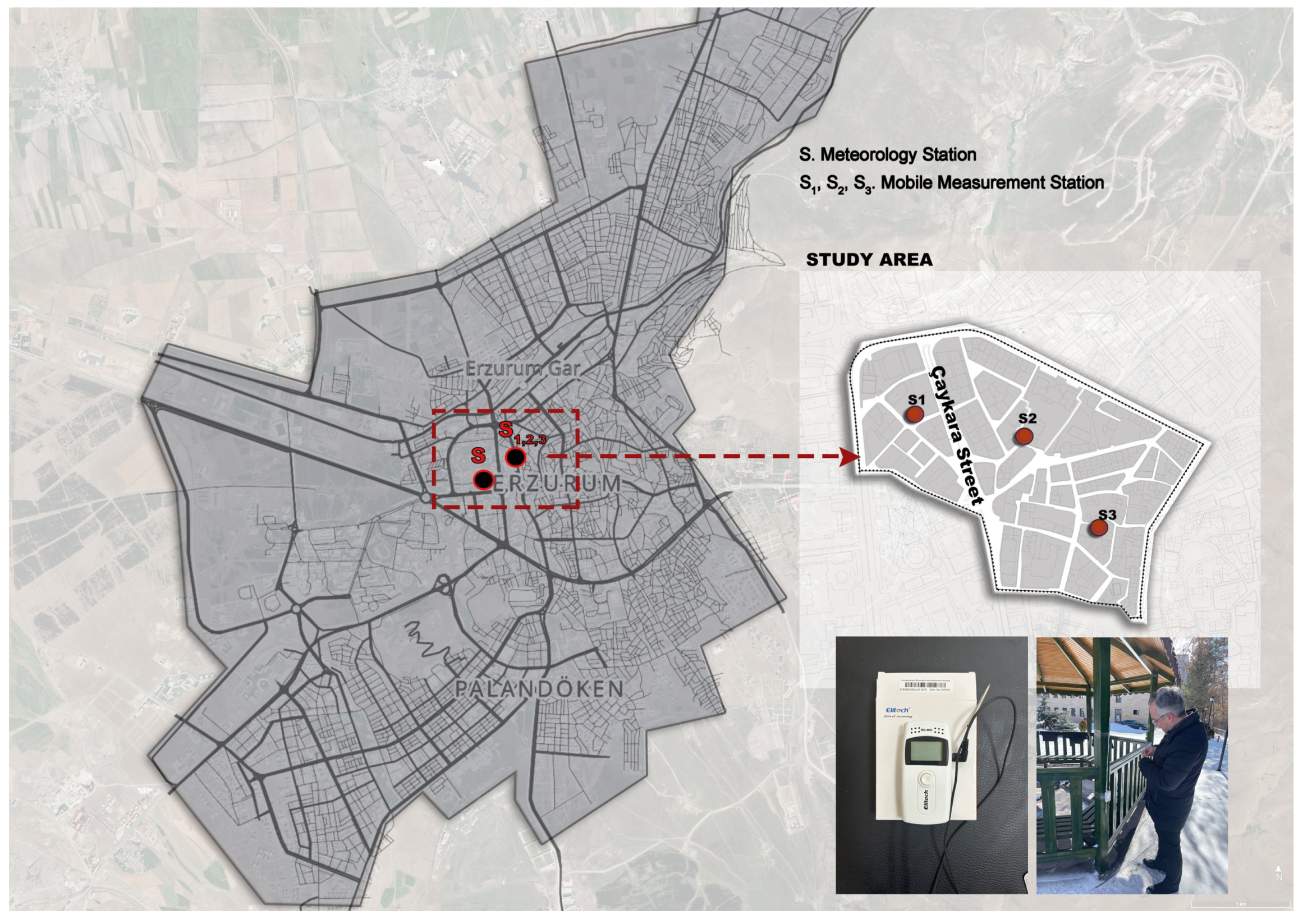
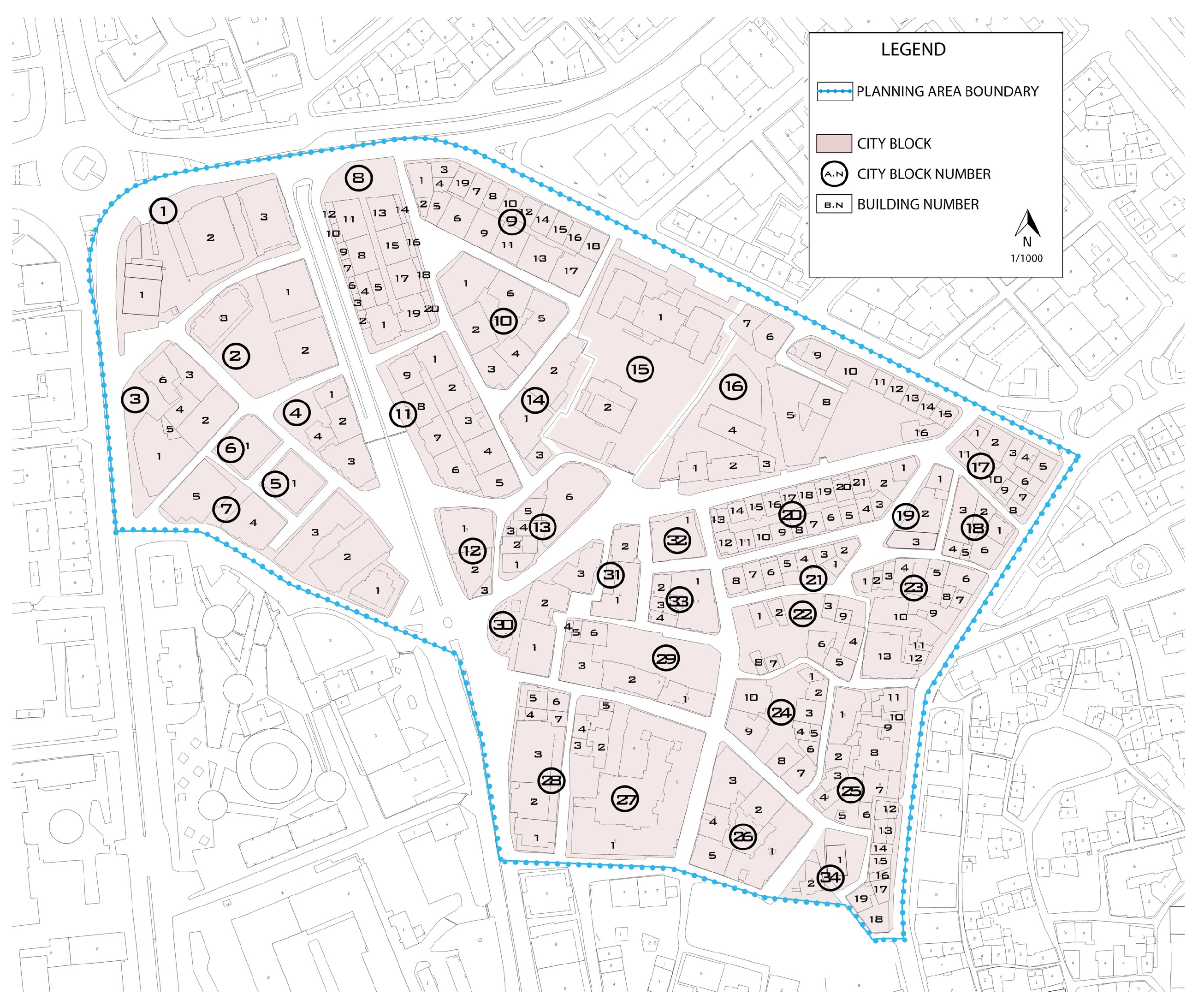
The study focuses on Çaykara Street in Erzurum, an area with a mix of residential and commercial functions located in the center of the city, as shown in Figure 1. The southern part of the area, up to Cumhuriyet Street, was excluded from the study due to the presence of public buildings and irregular construction subject to urban transformation. The study is limited to examining the change in microclimate and heating and cooling loads of buildings if the covered Çaykara Stream were to be opened.

The meteorological data of the city, along with the physical characteristics of the study area, constitute the primary material of the project. The selection of the climate data to be used and a representative simulation period is of great importance for the design recommendations to be made. The study area has a humid continental climate with cold, snowy days. However, the study did not consider the winter period alone. This is because the area experiences a high number of sunny days, particularly during the summer period. Additionally, the high-altitude effect and urban heat island effect contribute to high temperatures. Hourly temperature (°C) measurements for summer (June, July, August) and winter periods (December, January, February) in the study area were recorded with a digital heat and humidity measuring device of the Elitech model. The devices were taken to the Erzurum Meteorology Regional Directorate and operated there for one day with the assistance of a technical team to calibrate them. In addition, meteorological data, including air temperature (Ta; °C), wind speed (w/v; m/s), wind direction, and relative humidity (RH; %), were collected hourly for the same days from the official meteorological station (Regional Directorate of Meteorology of Turkish State Meteorological Service in Erzurum) located 450 m from the study area.

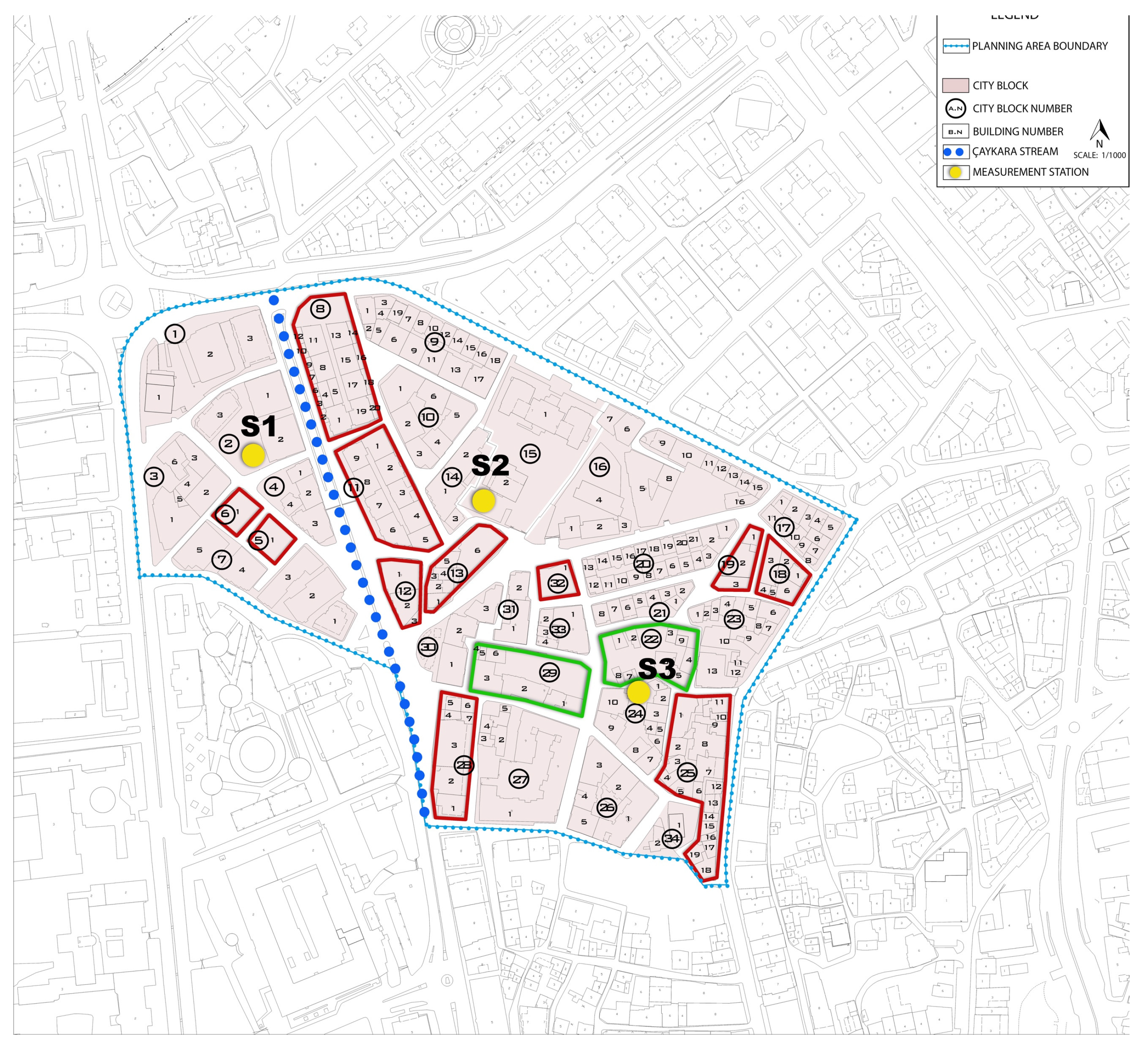
It is important to choose a location that best represents the character and climate of the region. Although there is no standard for inter-station distances horizontally, it can be seen in the literature that the intervals are based on an average of 500 m⁻¹ km. However, in terms of identifying different land uses in the microclimate, more frequently located stations allow for more data comparisons. Therefore, in order to better understand the microclimate of the study area, mobile measuring devices recording temperature data were positioned at an average height of 2 m above the ground, at an interval of 200 m, and at 3 points 50 m (S1), 100 m (S2), and 150 m (S3) away from the street to test the heating/cooling effect of the flow (Figure 1).

In order to verify the baseline value in the study area, the microclimate data measured manually (S1, S2, and S3) were compared with the data taken from the meteorological station (S) 450 m away from the study area during the same period (

Table 2. Recorded temperature data (°C).

Month of Measurement		Mobile Measurement Stations Average (S1, S2, S3)	Meteorological Station (S)	Difference
June 2022	Temperature (°C)	17.6	16.6	1
	Humidity (%)	48.6	60.9	−12.3
July 2022	Temperature (°C)	21.7	20.5	1.2
	Humidity (%)	41.2	48.3	−7.1
August 2022	Temperature (°C)	24.1	23.1	1
	Humidity (%)	32.1	37.3	−5.2
December 2022	Temperature (°C)	−0.7	−0.8	0.1
	Humidity (%)	68.1	78.9	−10.8
January 2023	Temperature (°C)	−2.5	−3.9	−1.4
	Humidity (%)	59.9	63.6	−3.7
February 2023	Temperature (°C)	−5.6	−7.8	−2.2
	Humidity (%)	55.4	68.7	−13.3

). The results showed that the measurements taken during this month were found to be close to the Erzurum average. Additionally, August had the highest average temperature during the summer period, while, for the winter period, the coldest average temperature was found in February. Therefore, August and February were selected for measurement.

To determine the hottest day in August and the coldest day in February, we compared the daily average temperatures of the measurement stations. We excluded the first day of the month from the ranking as it was the starting day of the measurement. We then identified the 15th day with the highest values in August and the 12th day with the lowest value in February as simulation days (

Table 3. Daily average temperature data for August 2022 and February 2023 (°C).

	August 2022			February 2023
Day	(S1)	(S2)	(S3)	(S1)	(S2)	(S3)
1	27.07	29.47	27.18	−0.50	−2.38	−1.49
2	23.67	26.37	23.58	−1.94	−3.68	−3.10
3	24.28	26.33	23.98	−4.73	−7.51	−7.10
4	24.53	26.60	24.27	−6.35	−9.10	−7.93
5	25.06	26.81	24.93	−3.71	−5.77	−5.41
6	23.10	25.24	22.86	−0.62	−2.06	−1.80
7	23.13	25.21	22.90	−0.94	−2.83	−2.46
8	21.97	23.73	21.99	−4.02	−6.74	−6.59
9	22.78	24.19	22.78	−7.10	−10.16	−9.61
10	23.25	24.22	23.13	−10.65	−8.79	−8.25
11	23.77	25.08	23.55	−13.53	−11.53	−11.24
12	23.42	24.95	23.24	−14.53	−12.54	−12.24
13	23.69	24.77	23.63	−14.49	−12.68	−12.10
14	25.15	26.23	24.97	−14.23	−12.63	−12.08
15	25.13	27.07	25.09	−12.73	−11.40	−11.28
16	24.18	26.13	23.95	−9.47	−8.65	−8.08
17	24.58	26.40	24.65	−7.59	−6.66	−6.11
18	24.38	26.17	24.35	−8.80	−7.64	−7.15
19	23.62	24.99	23.59	−3.06	−2.52	−2.03
20	23.22	24.55	23.22	−0.08	0.25	0.72
21	23.38	24.19	23.24	−1.72	−0.94	−0.43
22	22.27	22.87	22.02	−0.27	0.32	0.58
23	22.62	23.55	22.54	0.58	1.08	1.61
24	23.20	23.78	23.07	−5.50	−4.45	−3.80
25	23.98	24.65	23.73	−6.11	−4.11	−3.82
26	24.73	25.52	24.47	−2.81	−1.75	−1.71
27	24.70	25.49	24.62	−2.55	−1.57	−1.22
28	23.12	24.39	23.35	−1.65	−0.52	−0.46
29	22.15	23.70	22.31
30	23	24.42	22.97
31	24	25.27	23.98

). In the ENVI-met model, simulations can be analyzed using at least 24 h of meteorological data [37].

Table 4. 15 August 2022 meteorological data.

Date	Time	Air Temperature (°C)	Relative Humidity (%)	Wind Speed (m/s)	Wind Direction
15 August 2022	06:00	22.5	37.3	1.2	50°
15 August 2022	07:00	25.5	37.4	2.1	90°
15 August 2022	08:00	28.2	37.5	3.1	300°
15 August 2022	09:00	29.3	36	3.6	350°
15 August 2022	10:00	31.2	32.2	2.6	99°
15 August 2022	11:00	30.5	31.2	3.6	230°
15 August 2022	12:00	33.2	28.4	5.1	210°
15 August 2022	13:00	32.2	24.6	4.1	99°
15 August 2022	14:00	32	20	4.6	230°
15 August 2022	15:00	31.9	17.4	4.1	220°
15 August 2022	16:00	32.3	18.6	3.6	230°
15 August 2022	17:00	32.7	18.6	3.1	210°
15 August 2022	18:00	28.3	20.9	1.5	210°
15 August 2022	19:00	26.8	23.2	2.1	270°
15 August 2022	20:00	25.9	25.4	2.6	290°
15 August 2022	21:00	29.6	27.7	1.0	50°
15 August 2022	22:00	29.8	27.6	1.0	99°
15 August 2022	23:00	23.2	29.8	1.0	99°
16 August 2022	00:00	22.5	30.3	2.6	80°
16 August 2022	01:00	27.7	31.4	0.5	99°
16 August 2022	02:00	26.9	31.9	0	0°
16 August 2022	03:00	26.5	33.5	0.5	270°
16 August 2022	04:00	26	34.5	0.5	99°
16 August 2022	05:00	19.6	32.9	0.5	99°
16 August 2022	06:00	20.9	31.2	1.0	340°
16 August 2022	07:00	24.2	32.9	1.5	360°
16 August 2022	08:00	26.9	34.1	2.1	99°
16 August 2022	09:00	27.6	35.3	2.6	10°
16 August 2022	10:00	29.9	32.1	3.1	310°
16 August 2022	11:00	29.5	30	2.1	99°

and

Table 5. 12 February 2023 meteorological data.

Date	Time	Air Temperature (°C)	Relative Humidity (%)	Wind Speed (m/s)	Wind Direction
12 February 2023	06:00	−15.3	51.3	0.0	0°
12 February 2023	07:00	−16.2	51.8	0.5	300°
12 February 2023	08:00	−15.4	52.2	0.5	260°
12 February 2023	09:00	−13.1	54.9	0.5	320°
12 February 2023	10:00	−13.4	49.9	0.5	250°
12 February 2023	11:00	−8.3	50.5	0.5	280°
12 February 2023	12:00	−6.8	48.7	0.5	260°
12 February 2023	13:00	−4.6	36.3	0.5	290°
12 February 2023	14:00	−6.6	37.5	0.5	250°
12 February 2023	15:00	−8.4	36.9	0.5	270°
12 February 2023	16:00	−10.7	37.5	0	0°
12 February 2023	17:00	−11.1	38.4	0	0°
12 February 2023	18:00	−12.8	39.7	0	0°
12 February 2023	19:00	−13.3	41	0	0°
12 February 2023	20:00	−15.6	42	0	0°
12 February 2023	21:00	−13.8	43.3	0	0°
12 February 2023	22:00	−15.9	43.1	0	0°
12 February 2023	23:00	−16.3	45.5	0	0°
13 February 2023	00:00	−16.8	45.5	0	0°
13 February 2023	01:00	−16.4	46.4	0	0°
13 February 2023	02:00	−16.6	46.8	0	0°
13 February 2023	03:00	−17.1	47.2	0	0°
13 February 2023	04:00	−18.2	45.8	0	0°
13 February 2023	05:00	−17.8	46.8	0	0°
13 February 2023	06:00	−16.3	50	0	0°
13 February 2023	07:00	−11.7	48.4	0.5	260°
13 February 2023	08:00	−13.8	48.4	0.5	280°
13 February 2023	09:00	−11.4	48.9	0.5	40°
13 February 2023	10:00	−9.5	39.1	0.5	40°
13 February 2023	11:00	−8	39.4	0.5	10°

provide information on hourly meteorological data. Wind measurements were obtained from the meteorological station (S). The prevailing wind direction is southwest [36]. Since Erzurum city centre is located on a plateau, the average annual wind speed is low (2.7 m/s). In particular, December (2.1 m/s), February (2.3 m/s), and January (2.1 m/s) are the months with the lowest wind speed, respectively [38].

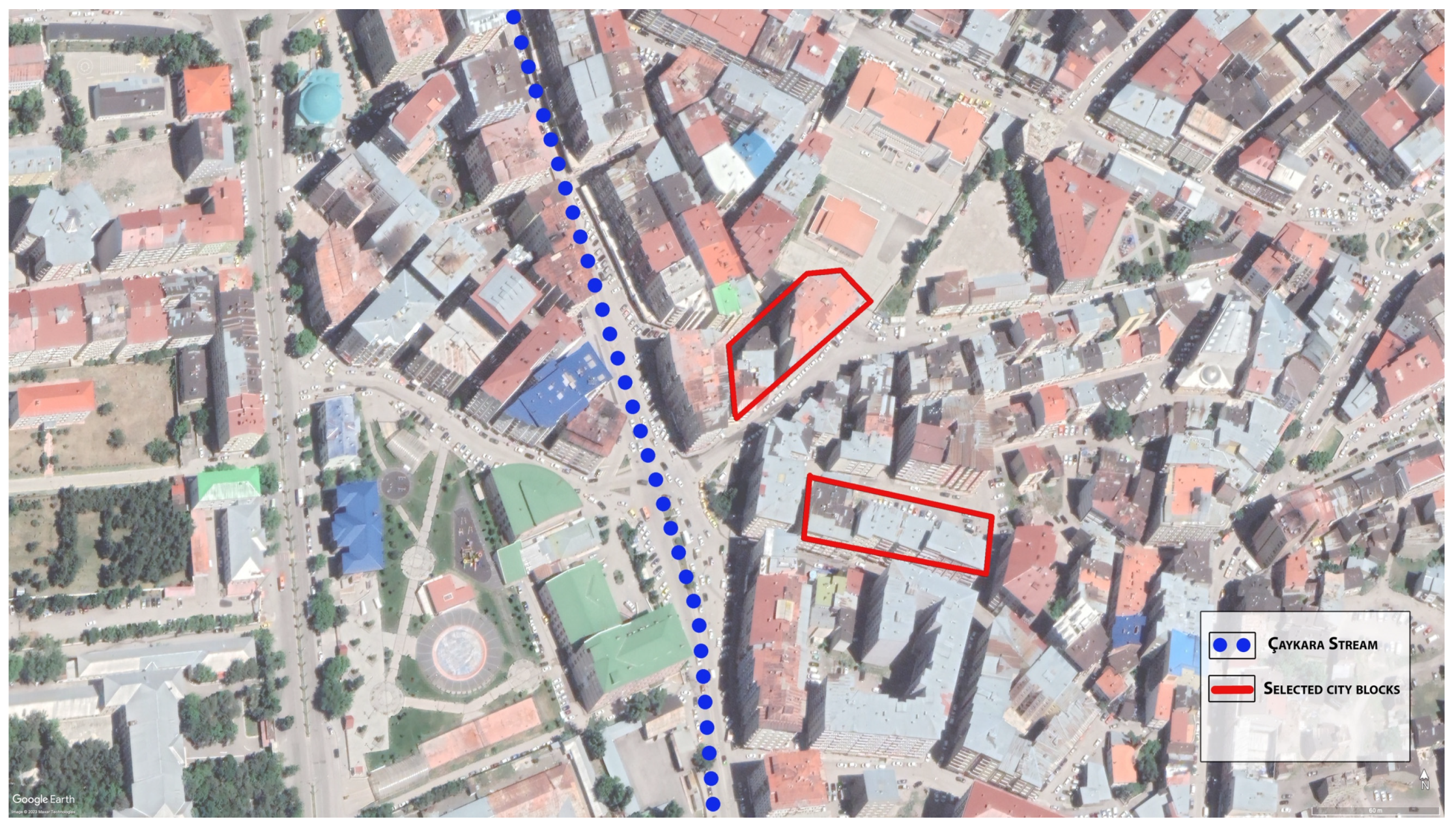
Doğanay [39] identified the Çaykara Stream Valley and the stream bed as one of the sides of the valley floor within the city where spring water fountains were collected (Figure 2). Today, however, Çaykara Stream, which runs through the city and is designated as the study area within the scope of the research, has been covered over, and the southern part of the stream has been turned into residential and commercial areas, while the north has been turned into a road called Çaykara Street today. This street is located in the city center and experiences high volumes of both vehicle and pedestrian traffic. It has dense, hard surfaces and experiences decreased air quality, particularly in winter. Thus, the street provides an ideal location to detect microclimate changes. The decision to choose this street was also influenced by the consistent distance between buildings, which ranges from 20 to 72 m.

Physical analysis and meteorological data of the study area provided two important datasets as the material to be used. For the physical analysis, the occupancy patterns and gross area data of the structures were collected and modeled to achieve total heating/cooling load reduction in an area of approximately 10 hectares. In addition, the total built area’s building coverage ratio (BCR) and floor area ratio (FAR), height/width ratio (H/W), orientation, impervious hard surface, and pervious surface (green area) ratios were all computed.

3.2. Methodology

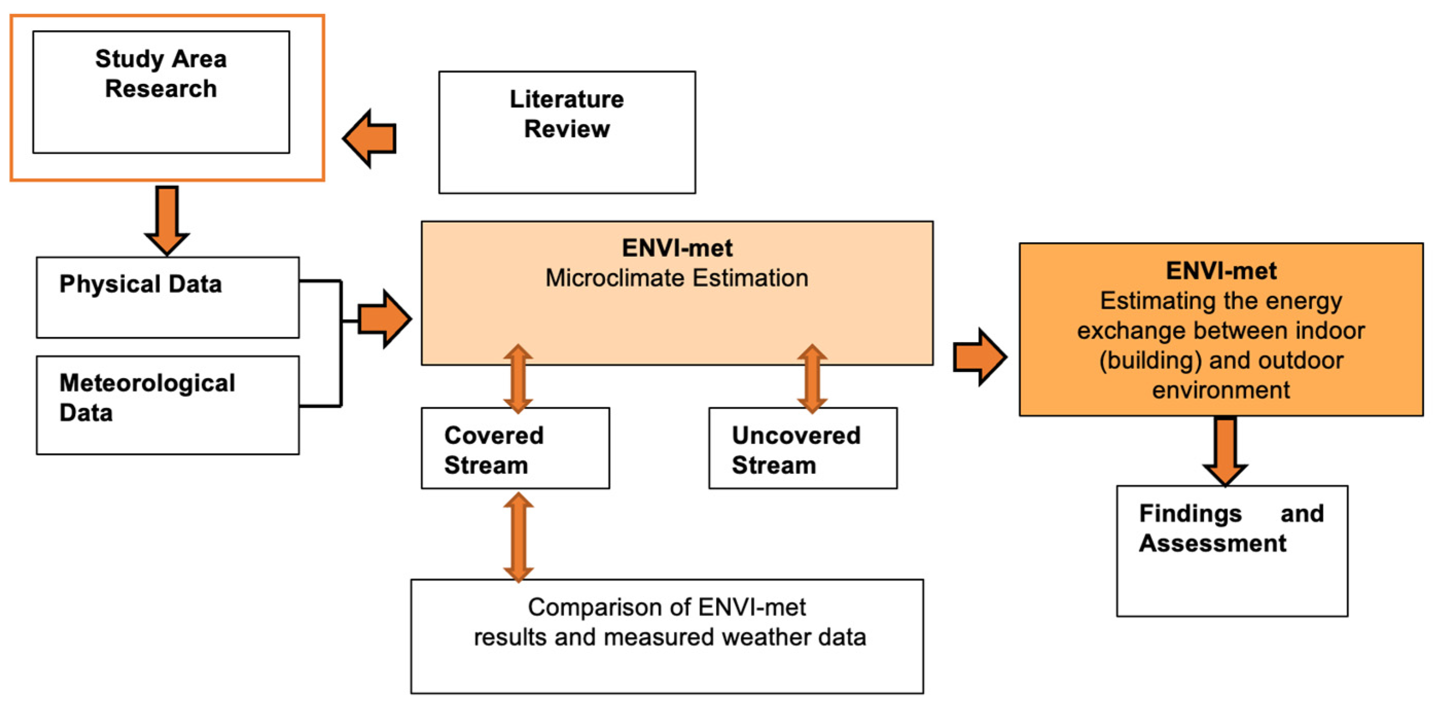
The study’s methodology involves creating microclimate simulation maps using recorded and calculated data, including meteorological data such as air temperature (°C), relative humidity (g/m³), average reflected temperature (°C), wind speed (m/s) and direction, and physical data along a selected covered stream bed line as a reference point in the city center of Erzurum, and researching the change in energy load of buildings accordingly (Figure 3).

This study utilized ENVI-met, a microclimate prediction program developed by Bruse [41,42] to evaluate the microclimate changes resulting from the transformation of the stream line. Additionally, the program was used to calculate the PET (physiological equivalent temperature) thermal comfort value, which is one of the thermal comfort indices. PET is based on a prognostic model of the human energy balance that calculates the skin temperature, body core temperature, sweat rate, and clothing temperature. The model is based on the 2-node model proposed by Gagge et al. [43] and was compiled and extended by Höppe [44] to the Munich Energy Balance Model for Individuals (MEMI). For PET, only the stationary solution of the body parameters is used, although the core model can be applied to both instationary and stationary approaches. Six parameters are utilized to calculate PET: Air temperature, average reflected temperature, wind speed, relative humidity, metabolic rate, and thermal insulation of clothing. The PET value is categorized under a nine-point psychophysical scale ranging from 4 °C to 41 °C (

Table 6. PET index thermal stress categories [43].

PET (°C)	Thermal Perception	Grade of Physiological Stress
<4.0	Very cold	Extreme cold stress
4.1–8.0	Cold	Strong cold stress
8.1–13.0	Cool	Moderate cold stress
13.1–18.0	Slightly cool	Slight cold stress
18.1–23.0	Comfortable	No thermal stress
23.1–29.0	Slightly warm	Slight heat stress
29.1–35.0	Warm	Moderate heat stress
35.1–40.0	Hot	Strong heat stress
>41.0	Very hot	Extreme heat stress

). The values in Table 6, used for the evaluations in this study, include the values obtained by Matzarakis et al. [45] based on an average European man.

Due to the large number of buildings in the area, estimating the energy load of each building can be challenging. In physical data analysis and building area research, buildings are often categorized to simplify the process. The categories are listed below:

• Classification by building utilization (retail, restaurant, residential, hotel, office)
• Classification by construction period (before 1970s, 1970s to 1980s, after 1980)
• Classification according to gross area regardless of building floor area or number of floors

Furthermore, the study did not use the classification based on building structure, as the difference in structure was described due to a single factor. It is important to note that the wall supporting the buildings has a significant impact on thermal load and typically exhibits common features based on the construction period.

Additionally, the ENVI-met simulation program used in the study calibrated the measured and simulated data to increase result reliability. One alternative approach is to verify the absolute value of all ENVI-met results. However, the method selected in this study provides an objective comparison of the effects of urban measures. Therefore, when the same input parameters are used for all simulations, differences in real-time weather conditions or climate become insignificant.

3.2.1. Using ENVI-Met Microclimate Model

ENVI-met v5.5.1. is a three-dimensional microclimate simulation (CFD) software. It considers total radiation and uses fluid dynamics and thermodynamics laws to model the evolution of climate variables. The model calculates the atmosphere’s state by combining the influence of buildings, vegetation, surface features, soils, and climatic conditions [44]. In addition, when the relationship of the program with the microclimate on a building basis is analyzed, it is evident that significant feedback has been obtained. The model considers the complex and dynamic environment formed by buildings, the urban environment, green areas, and traffic infrastructure. The holistic and high-resolution approach of ENVI-met allows for simulation of energy flows at the façade scale of a single building and the microscale urban metabolism as a complex system (Figure 4) [46].

ENVI-met was chosen for this investigation because of its ease of use and dependability in measuring urban microclimatic changes such as thermal comfort (PMV) and mean radiation temperature (TMRT). ENVI-met has been rigorously tested for evaluating urban design solutions in outdoor thermal settings [47,48,49,50,51,52]. It outperforms other methods for predicting urban microclimate conditions as the best model for assessing human comfort at street level.

ENVI-met requires several input parameters, including meteorological data, initial soil structure and temperature profiles, the structure and properties of ground surfaces, vegetation elements, and buildings. To run the simulation, two user-generated files are required: An area input file in *.INX format, which contains physical information about the simulated area, including dimensions, building size, surface materials, roads, and vegetation. The ENVI-met program also requires climatic data such as temperature, humidity, wind speed, and direction from mobile measurements or a fixed meteorological station to start a simulation. This data is stored in a *.SIM file and is linked to the field input file (*.INX), soil database, and plant database for the simulation run.

The model details the start date, run time, output interval, output folder location, timeout interval, starting point, meteorological parameters, radiation correction, and model timing. Grid size is crucial for evaluating thermal comfort with computer models, as it determines details for modeling buildings, spatial locations, and distances between calculated points. ENVI-met has a minimum and maximum grid size of 0.5 × 0.5 mm and 10 × 10 m, respectively.

3.2.2. Data Input and Simulation Process

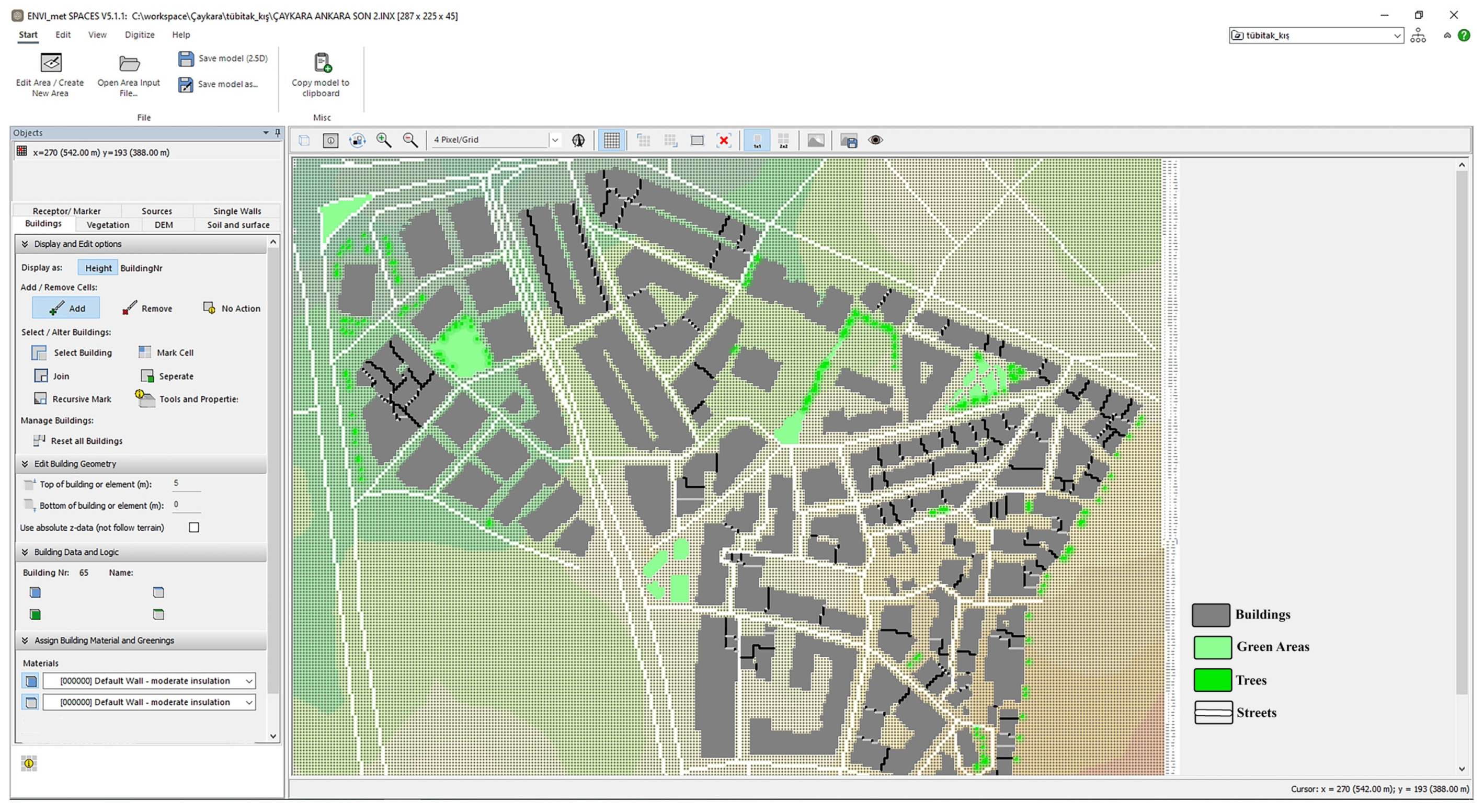
The simulations in this study were performed using ENVI-met v5.5.1. Each grid in the study area represents an area of 2 m × 2 m, with a total of 45 grids in the Z direction and a model height of 90 m. The area input file (.INX) has a grid cell of 287 × 225 × 45 (x × y × z), with a grid size of 12 × 2 × 2 m (x × y × z), resulting in an area size of 574 × 450 × 90 m (Figure 5 and Figure 6).

It should be noted that in ENVI-met simulations, the meteorological input data does not directly correspond to a specific date. The important point is to prevent extreme temperatures from creating bias and to ensure that the simulation result reflects the average temperature during the specified hours. Thus, the climate file in the study is of a two-seasonal period, and not of a single day to prevent extreme conditions from occurring.

Table 7. Simulation input data.

Location	Erzurum/Çaykara
Measurement Period	Summer	Winter
Simulation Initialization and Properties
Initial day of simulation	15 August	12 February
Initial hour of simulation	05:00	05:00
Total simulation time (hour)	30	30
Grid cell (x, y, z)	287 × 225 × 45	287 × 225 × 45
Grid size (meters) (x, y, z)	2 × 2 × 2	2 × 2 × 2
Model rotation	0	0
Meteorological Conditions
Wind speed (m/s)	0.5	0.5
Wind direction (0:N, 90:E, 180:S, 270:W)	250°	200°
Roughness at reference point (m)	0.1	0.1
Initial temperature (°C)	20.8	−15.3
Specific humidity (2500 m) (g water/kg air)	7.0	7.0
Relative humidity (2 m) (%)	36.4	51.3

shows the input data used in the simulation. Since the model requires an accurate initialization time, and the first 6 h of output are considered the turnaround time of the model, it was run for a total of 30 h.

In the literature, it is emphasized that the midday hours cause more heat accumulation in urban areas [10,11,28]. In particular, the range of thermal comfort values increases at midday. It is therefore expected that a wider range will show more detail and allow for a more accurate comparison between variables. For this reason, the results are compared according to the values at 13:00.

After employing the simulation data on ENVI-met, a spatial analysis was made for the selected research area in order to understand the existing microclimate factors within and select the appropriate building blocks to evaluate the impact of the opening of covered water surfaces. Then, simulations were made for the analysis of microclimatic and thermal comfort changes in the research area after the rehabilitation of water surfaces for both the winter and summer seasons. The last simulations aimed to calculate the temperature differences on the façade of buildings through the selected building blocks in the research area.

3.2.3. Validation of Simulations

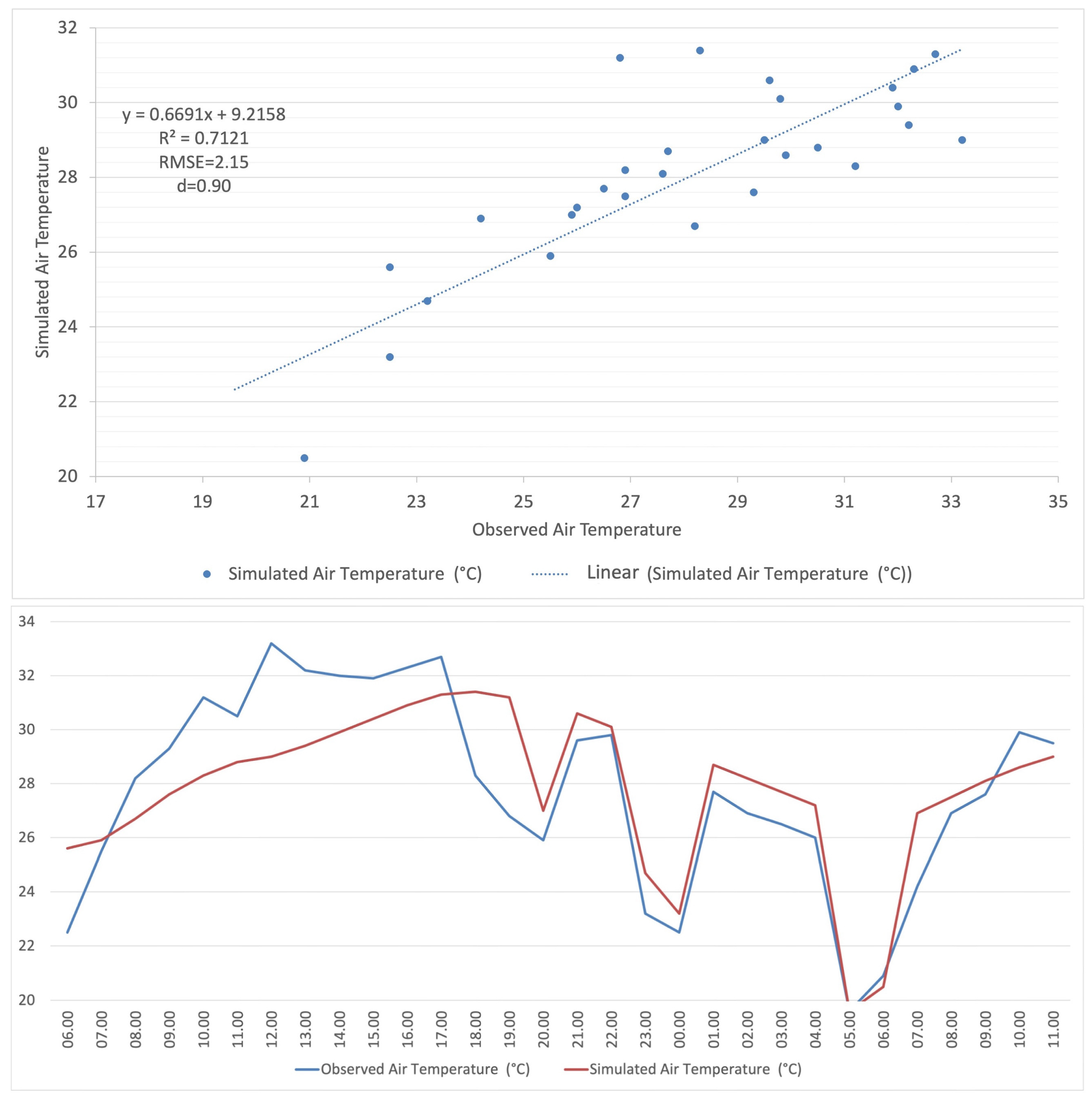
This study aimed to calibrate a simulation model by comparing its output with actual measured data from a weather station. The model’s accuracy was assessed using two indicators [53]: The root-mean-square error (RMSE) and the index of agreement (d) (Figure 7). The performance of the model was evaluated by measuring the difference between simulated and observed air temperature. The agreement index (d) is a descriptive measure used to evaluate the accuracy of simulated values, ranging from 0 to 1, with 1 indicating absolute agreement. The closer the d value is to 1, the more accurate the modeling results. Another indicator, RMSE, is a measure that compares different prediction errors in a dataset and indicates accuracy. Smaller values indicate less error in prediction.

The study compares daily air temperatures simulated with ENVI-met with data measured on 15 August 2022, and 12 February 2023. The graphs show that the increase and decrease in air temperatures occur at the same time of the day. The agreement index between the simulated and measured air temperature during the summer period was 0.90, with an RMSE value of 2.15 over a 30 h period. Similarly, during the winter period, the agreement index was 0.95 with an RMSE value of 1.84 (

Table 8. Evaluation of measured and simulated temperatures in August 2022.

Date	Time	Observed Air Temperature	Simulated Air Temperature	Difference	Difference Square	Index of Agreement (d)
15 August 2022	06:00	22.5	25.6	3.10	9.61	0.904007072
15 August 2022	07:00	25.5	25.9	0.40	0.16
15 August 2022	08:00	28.2	26.7	−1.50	2.25
15 August 2022	09:00	29.3	27.6	−1.70	2.89
15 August 2022	10:00	31.2	28.3	−2.90	8.41
15 August 2022	11:00	30.5	28.8	−1.70	2.89
15 August 2022	12:00	33.2	29	−4.20	17.64
15 August 2022	13:00	32.2	29.4	−2.80	7.84
15 August 2022	14:00	32	29.9	−2.10	4.41
15 August 2022	15:00	31.9	30.4	−1.50	2.25
15 August 2022	16:00	32.3	30.9	−1.40	1.96
15 August 2022	17:00	32.7	31.3	−1.40	1.96
15 August 2022	18:00	28.3	31.4	3.10	9.61
15 August 2022	19:00	26.8	31.2	4.40	19.36
15 August 2022	20:00	25.9	27	1.10	1.21
15 August 2022	21:00	29.6	30.6	1.00	1
15 August 2022	22:00	29.8	30.1	0.30	0.09
15 August 2022	23:00	23.2	24.7	1.50	2.25
16 August 2022	00:00	22.5	23.2	0.70	0.49
16 August 2022	01:00	27.7	28.7	1.00	1
16 August 2022	02:00	26.9	28.2	1.30	1.69
16 August 2022	03:00	26.5	27.7	1.20	1.44
16 August 2022	04:00	26	27.2	1.20	1.44
16 August 2022	05:00	19.6	19.6	0	0
16 August 2022	06:00	20.9	20.5	−0.40	0.16
16 August 2022	07:00	24.2	26.9	2.70	7.29
16 August 2022	08:00	26.9	27.5	0.60	0.36
16 August 2022	09:00	27.6	28.1	0.50	0.25
16 August 2022	10:00	29.9	28.6	−1.30	1.69
16 August 2022	11:00	29.5	29	−0.50	0.25

and

Table 9. Evaluation of measured and simulated temperatures in February 2023.

Date	Time	Observed Air Temperature	Simulated Air Temperature	Difference	Difference Square	Index of Agreement (d)
12 February 2023	06:00	−15.3	−15.6	−0.30	0.09	0.951101858
12 February 2023	07:00	−16.2	−15.8	0.40	0.16
12 February 2023	08:00	−15.4	−15.6	−0.20	0.04
12 February 2023	09:00	−13.1	−15.4	−2.30	5.29
12 February 2023	10:00	−13.4	−15.1	−1.70	2.89
12 February 2023	11:00	−8.3	−8	0.30	0.09
12 February 2023	12:00	−6.8	−6.8	0	0
12 February 2023	13:00	−4.6	−4.6	0	0
12 February 2023	14:00	−6.6	−6.5	0.10	0.01
12 February 2023	15:00	−8.4	−9.5	−1.10	1.21
12 February 2023	16:00	−10.7	−14.7	−4.00	16
12 February 2023	17:00	−11.1	−14.9	−3.80	14.44
12 February 2023	18:00	−12.8	−15	−2.20	4.84
12 February 2023	19:00	−13.3	−13.1	0.20	0.04
12 February 2023	20:00	−15.6	−14.2	1.40	1.96
12 February 2023	21:00	−13.8	−13.3	0.50	0.25
12 February 2023	22:00	−15.9	−15.4	0.50	0.25
12 February 2023	23:00	−16.3	−15.5	0.80	0.64
13 February 2023	00:00	−16.8	−16.6	0.20	0.04
13 February 2023	01:00	−16.4	−15.7	0.70	0.49
13 February 2023	02:00	−16.6	−15.8	0.80	0.64
13 February 2023	03:00	−17.1	−16	1.10	1.21
13 February 2023	04:00	−18.2	−16.1	2.10	4.41
13 February 2023	05:00	−17.8	−16.2	1.60	2.56
13 February 2023	06:00	−16.3	−16.3	0	0
13 February 2023	07:00	−11.7	−11.4	0.30	0.09
13 February 2023	08:00	−13.8	−13.1	0.70	0.49
13 February 2023	09:00	−11.4	−15.8	−4.40	19.36
13 February 2023	10:00	−9.5	−9.6	−0.10	0.01
13 February 2023	11:00	−8	−10	−2	4

; Figure 8 and Figure 9).

4. Results

In order to verify the heat island density and the initial value in the study area, the microclimate data manually measured hourly for 3 months for both winter (December–January–February) and summer (June–July–August) were compared with the hourly average weather data (meteorological station) of Erzurum during the same periods. In the data compared for the summer period, it was found that the highest average temperature belonged to the month of August. It was also observed that the measurements in this month were similar to Erzurum’s average. For the winter period, the coldest temperature average was found to belong to February, and these two months were selected for measurement. In this respect, the hottest day was determined by comparing the daily average temperatures of the measurement stations in August. The first day of the month was excluded from the ranking as it was the initial day of measurement, and the 15th day, which had the highest values after this day, was determined as the simulation day.

In the same way, the coldest day was determined by comparing the daily average temperatures of the measurement stations in February. The first day of the month was excluded from the ranking as it was the initial day of measurement, and the 12th day, which had the lowest values after this day, was determined as the simulation day.

4.1. Spatial Analysis Results of Study Area

The study area was divided into 34 city blocks, and a total of 245 buildings in the area were the subject of analysis (Figure 10).

The area was analyzed both on the basis of city blocks and buildings. For the block-specific analysis, 86.4% of the total area was calculated as impervious surfaces and 13.6% as previous surfaces (Figure 11 and Figure 12). The utilization, construction periods, and materials of the numbered buildings within each city block were identified (

Table 10. Buildings in the study area according to their functions.

Function of the Building	Residential	Commercial	Res. + Comm.	Touristic	Tour. + Comm.	Education	Worship	Auxiliary Buildings	Ruins
Number	59	46	111	8	8	2	5	3	3

,

Table 11. Number of different building materials used in the study area.

Building Materials (Number of Buildings)		Total Area Covered by Buildings (m2)	Area of Buildings by Gross Area (m2)
Masonry	Reinforced concrete	67.7	68,198
6	239

and

Table 12. Number of buildings in the study area by construction periods.

Building Construction Periods (Number of Buildings)
Before 1970	1970–1990	1990–2010	2010–2020
2	84	156	1

).

As mentioned in the Methodology section, several classifications were made to simplify the buildings and, as a result of the analysis, identify the buildings to be compared for simulation (

Table 13. Study area building BCR-FAR and city block hard floor ratios.

Number of City Blocks	BCR			FAR			Total Area (m2)	Impervious Surface Ratio (%)	Pervious Surface Ratio (%)
	0–0.20	0.20–0.30	0.30+	0–0.50	0.50–1.50	1.50+
1		X			X		5463	92.8	7.2
2		X			X		3879	80.3	19.7
3			X			X	3717	87.66	12.34
4		X			X		1555	87.14	12.86
5			X			X	782	100	0
6			X			X	920	100	0
7			X			X	5142	97.28	2.72
8			X			X	4375	100	0
9			X			X	4732	96.5	3.5
10			X			X	3190	97.9	2.1
11			X			X	4085	100	0
12			X			X	1363	100	0
13			X			X	2115	100	0
14			X			X	1930	95	5
15		X			X		7137	97.16	2.84
16			X			X	10,686	80.5	19.5
17			X			X	1860	98.9	1.1
18			X			X	1142	100	0
19			X			X	1046	100	0
20			X			X	2927	95	5
21			X			X	1355	96.8	3.2
22	X			X			2874	69.6	30.4
23			X			X	3000	72.79	7.21
24		X			X		2500	82.56	17.44
25			X			X	4000	100	0
26			X			X	3000	94.4	5.6
27		X			X		5000	100	0
28			X			X	2600	100	0
29	X			X			3500	71.43	28.57
30		X			X		2400	75	25
31			X			X	750	93.1	6.9
32			X			X	689	100	0
33			X			X	1000	100	0
34			X			X	1250	80.8	19.2
TOTAL							101,964	86.4	13.6

). First, a selection was made based on city blocks using permeable and impervious surface ratios and BCR/FAR values. Among the results, a grouping was made based on the “highest and lowest” values for these parameters in the area. For the pervious/impervious surface ratio, which defines the ratio of the area covered with hard (asphalt, stone, etc.) or pervious (soil) ground, the city blocks with the highest impervious surface ratio fell into the “negative” category, while the city blocks with a higher pervious surface ratio than the other city blocks fell into the “positive” category. In terms of building coverage ratio (BCR) and floor area ratio (FAR) ratios, the blocks with the lowest values were categorized as “positive” and the blocks with the highest values were categorized as “negative”. In line with the data obtained from Table 6 below,

• Blocks with a 100% impervious surface ratio (highest value)
• Blocks with a pervious surface ratio between 25 and 30% (highest value)
• Blocks with a BCR ratio between 0 and 0.20 and a FAR ratio between 0 and 0.50 (lowest values)
• Blocks with a BCR ratio of 0.30+ and a FAR ratio of 1.50+ (highest values) were selected.

As a result of the classification, blocks numbered 5, 6, 8, 11, 12, 13, 18, 19, 25, 28, and 32 were determined to be negative, while blocks numbered 22 and 29 were determined to be positive (

Table 14. Positive and negative city block groupings.

Negative	City Blocks with 100% Impervious Surface Ratio	Positive	City Blocks with 25–30% Pervious Surface Ratio
City blocks with a BCR ratio of 0.30+ and a FAR ratio of 1.50+	5, 6, 8, 11, 12, 13, 18, 19, 25, 28, 32	City blocks with BCR ratio between 0 and 0.20 and FAR ratio between 0 and 0.50	22, 29

and Figure 13). It should be noted that this classification is based on the comparison method. Otherwise, a 25–30% impervious surface ratio does not mean acceptable or good quality in basic urban planning principles.

Then, another selection was made among the blocks determined according to the functions of the buildings (retail, restaurant, residential, hotel, office) and construction period (before 1970s, from 1970s to 1980s, after 1980s). For this purpose, blocks grouped according to positive/negative attributes were overlaid with analyses based on land uses and construction periods (Figure 14, Figure 15 and Figure 16). While selecting buildings from two different block attributes, it was desired to have different examples within a block in terms of both building function and construction year. In addition, in line with the assumption of the uncovering of the covered Çaykara Stream, the proximity to the water and the presence of a similar city block on the front side of the two blocks also guided these choices. In this respect, it was decided to select the blocks numbered 13 and 29 and the buildings within them as the sample.

There are residential and commercial under residential classes as building utilization within the two blocks. In terms of construction years, there are 5 buildings constructed between 1970 and 1990 and one building between 1990 and 2010 on city block no. 13. On city block no. 29, there are 2 buildings constructed between 1970 and 1990 and 3 buildings constructed between 1990 and 2010.

4.2. Study Area Simulation Outputs

In this section, the impact of opening the covered stream line (Çaykara Stream) is evaluated through simulations. These simulations provided the analysis of microclimate change within the area selected during summer and winter separately, as well as the temperature differences on the facades of the above-selected buildings. Below, the results of the simulation analysis are given in comparison between the scenarios for the covered and uncovered situations of the stream in the summer and winter seasons.

4.2.1. Summer

Microclimate Change: In the simulations created for 15 August 2022 at 13.00 in the summer period, the microclimate change scenario that would occur with the uncovering of the Çaykara Stream was monitored. As can be seen in Figure 17, the average temperature in the area varied between 29.07 and 30.96 °C when there was no stream line, and the average temperature varied between 23.06 and 25.28 °C in the variation where the stream line was uncovered. Therefore, it can be inferred that uncovering the streamline will result in a temperature decrease of approximately 5 °C in the environment (see Figure 18).

It is evident that the areas between the buildings in the eastern part of the region are cooler due to the shadow effect. Additionally, the average air temperature dropped from 29.36 °C to 24.05 °C after the stream line was uncovered.

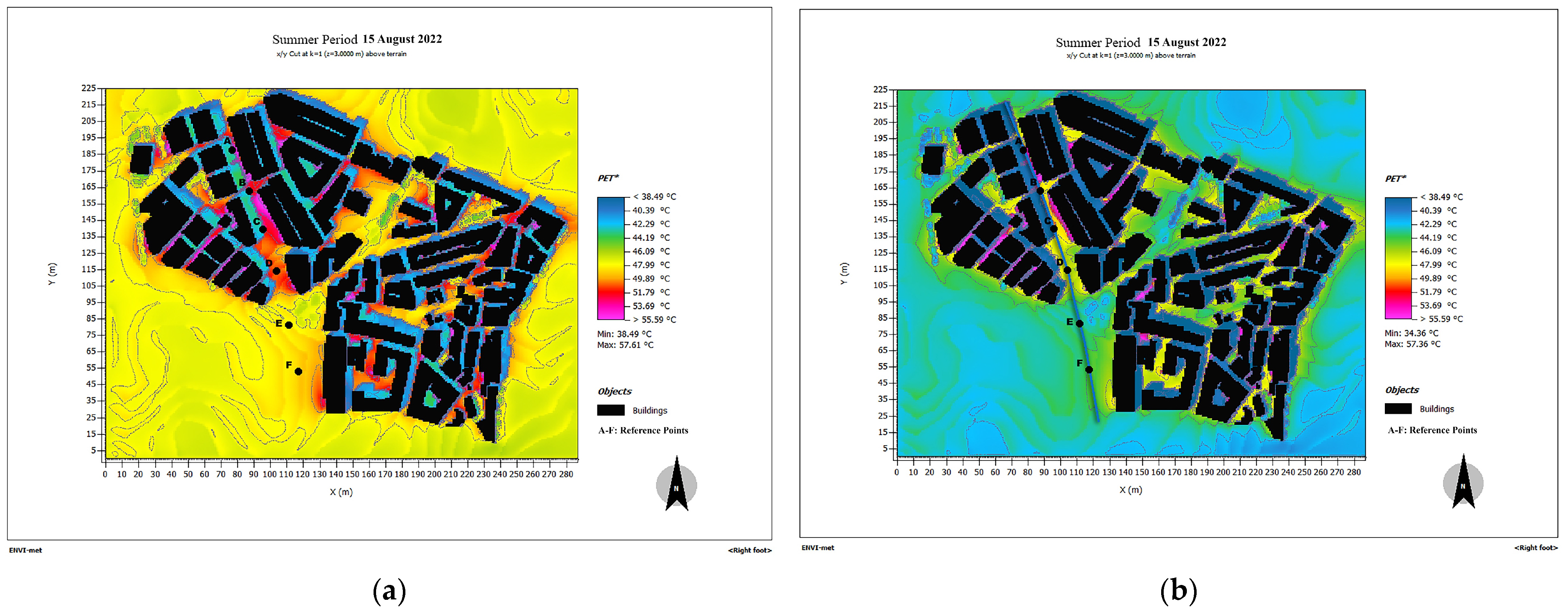
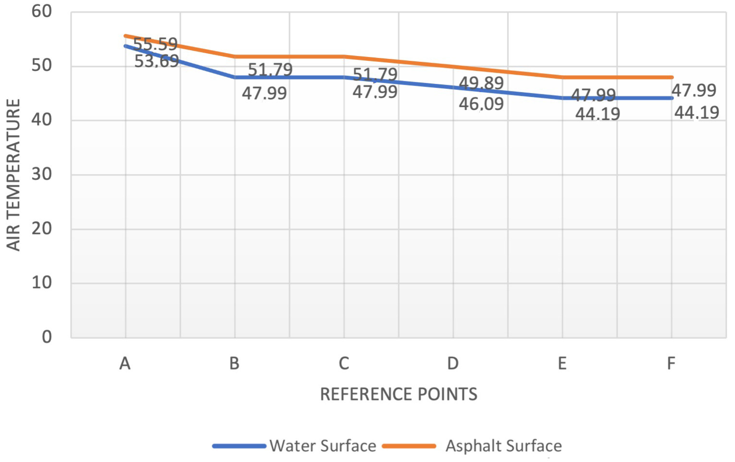
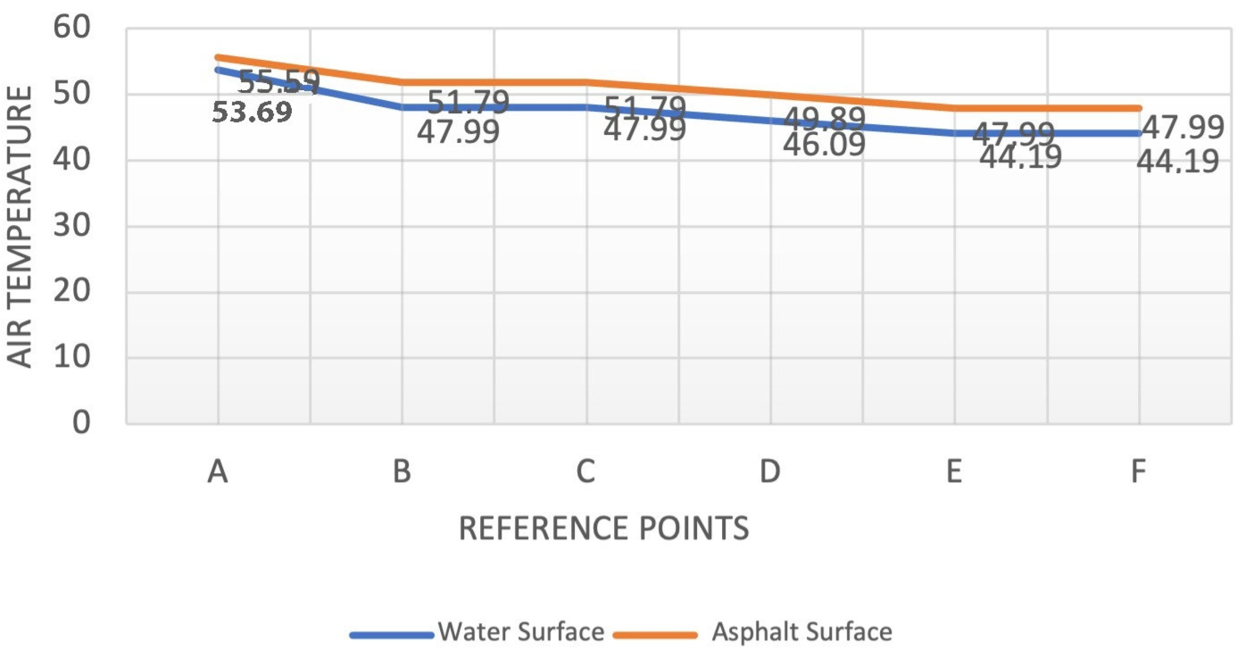
Thermal Comfort (PET) Variation: The comparative evaluation of the results for the PET values revealed that the thermal stress level for the summer was slightly lower under building shades and green areas (trees) but reached extreme heat stress in open and paved areas (Figure 19 and Figure 20). Especially in the variation where the stream bed was covered, points A, B, C, and D were at an alarming level between 51.79 °C and a maximum of 57.61 °C (Figure 19a). It can be seen that the presence of water increases the thermal comfort level throughout the area, i.e., it decreases the perceived temperature from a minimum of 38 °C to 34.36 °C (Figure 19b).

Sample Building-Based Changes: Simulation results of the selected city blocks (13 and 29) and buildings were analyzed in four different groups. These are:

• Exterior facade (wall) temperature
• Interior facade (wall) temperature
• Outdoor air temperature in front of the facade
• Building indoor temperature.

This section presents the maps and simulations for blocks 13 and 29, showing the temperature differences between the covered and uncovered states of the stream bed. The exterior facade (wall) temperature change ranges from 2.05 °C to 5.08 °C (Figure 21). The study found that uncovering the stream bed resulted in a decrease of up to 5 degrees Celsius in surface temperature on the roof. The north facade showed less difference due to the shadow effect, but still experienced a decrease between 2.65 and 3.26 degrees Celsius. Additionally, the study found that trees surrounding the buildings caused temperature drops on the facade, creating a cooling effect.

The simulation results indicate that the interior facade (wall) temperature varies between 0.12 °C and 1.23 °C (Figure 22). The highest temperature difference was observed in the interior facades of the buildings located along the uncovered stream. This suggests that the water flow causes an average temperature drop of 1 °C in these areas.

The temperature drops around the buildings between 5.13 °C and 5.73 °C with the uncovering of the stream line, which is also remarkable (Figure 23). The simulations indicate that the buildings with facades facing the uncovered stream area showed the highest difference, while the buildings on blocks numbered 13 and 29 had an average change of 5.46 °C.

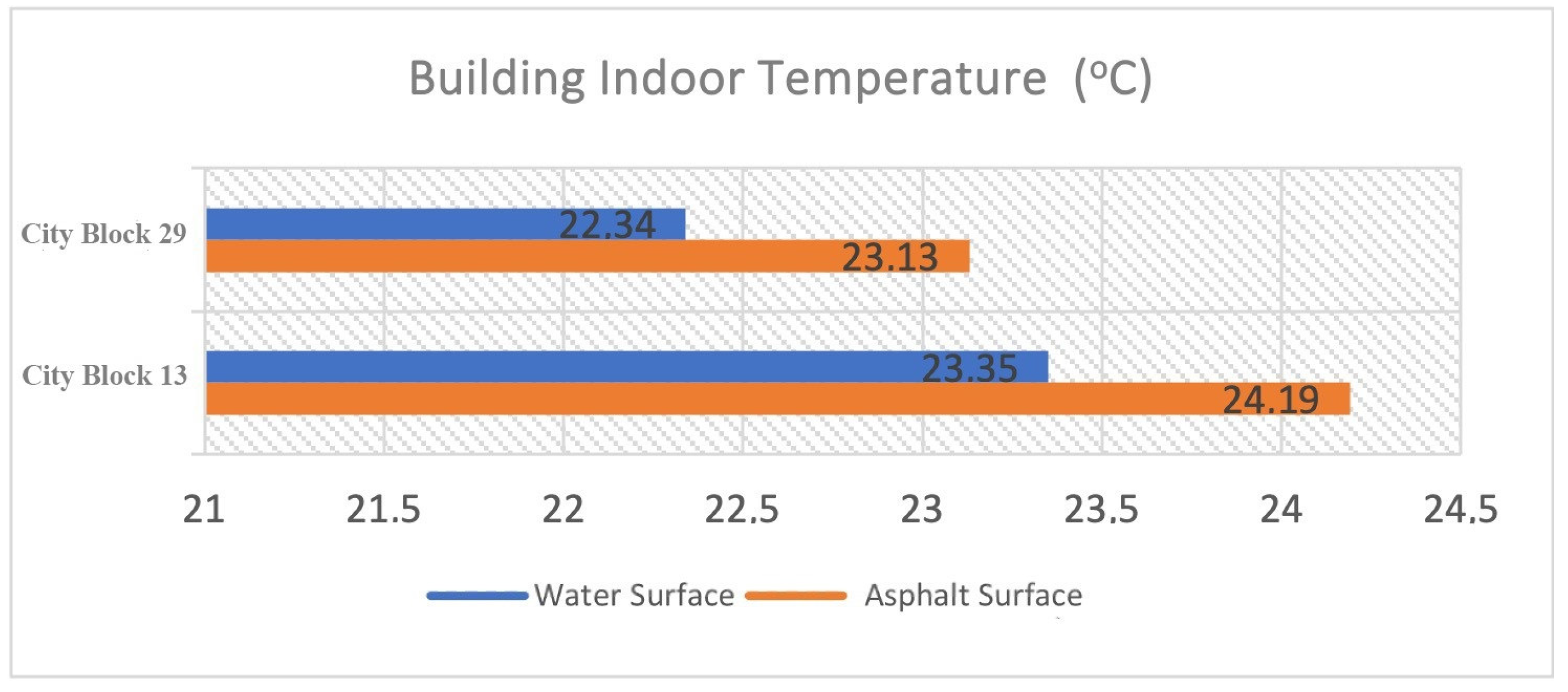
When analyzing the change in indoor temperature of the buildings, it can be observed that the water flow creates a cooling effect ranging from 0.13 °C to 0.99 °C. On average, a decrease of 0.7 to 0.8 °C was recorded for the sampled buildings on blocks numbered 13 and 29 (refer to Figure 24 and Figure 25).

4.2.2. Winter

Microclimate Change: The simulation for 12 February 2023 at 13:00 included monitoring the microclimate change scenario resulting from the uncovering of Çaykara Stream, as was conducted in the summer simulations. Figure 26a shows that the average temperature in the area ranged from −5.29 °C to −3.77 °C without the stream, while Figure 26b shows that the average temperature ranged from −5.27 °C to −3.76 °C when the stream was uncovered. According to Figure 26, the streamline will result in a temperature increase of around 0.02 °C in the area during the winter season.

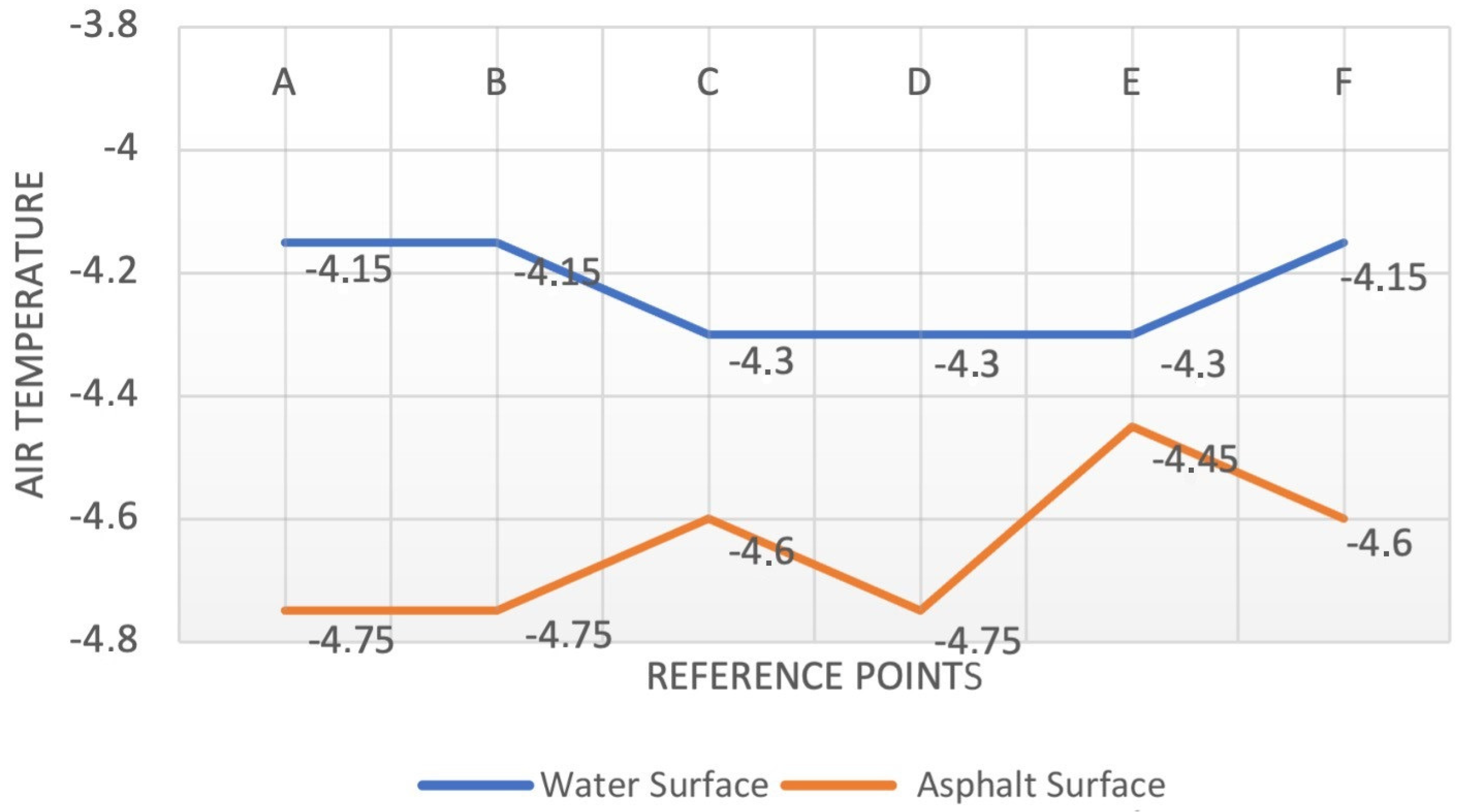
It is important to note, however, that, especially for the reference points along the streamline (A-B-C-D-E-F), there is a temperature increase of up to 0.6 °C at certain points (Figure 26 and Figure 27). The simulations indicate that water does not have a cooling effect in winter but rather creates a temperature increase in the microclimate along the stream line.

Thermal Comfort (PET) Change: The change in PET values in the area indicates that thermal comfort did not decrease despite winter conditions, but rather increased by 0.01–0.02 °C in the presence of water surface (Figure 28).

Sample Building-Based Changes: After uncovering the Çaykara Stream, the exterior (wall) temperature on 12 February 2023 showed a change ranging from −0.04 °C to 0.21 °C. The temperature increased by up to 0.16 °C, particularly on the 1st and 2nd floor exterior walls facing the stream line (Figure 29). Temperature increases of 0.08 °C were observed on the exterior facades near the stream on the 13th and 29th blocks, while increases of 0.01 °C were detected on the rear facades facing east.

The simulation results indicate a maximum increase of 0.06 °C in the interior facade (wall) temperature (Figure 30). The highest difference was detected, especially in the interior facades of the buildings on the route of the uncovered stream, while no difference was observed in other buildings. For the buildings on the 13th and 19th blocks, a maximum increase of 0.03 °C was observed on the interior facades close to the stream line.

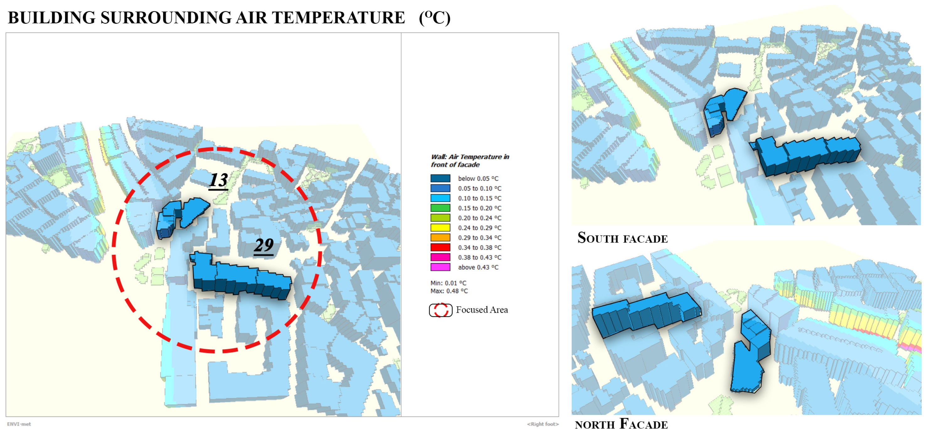
Regarding the change in air temperature around the building, the uncovered stream line route showed the highest increase (0.48 °C) compared to other areas (Figure 31). No changes in air temperature were detected in the other building surroundings.

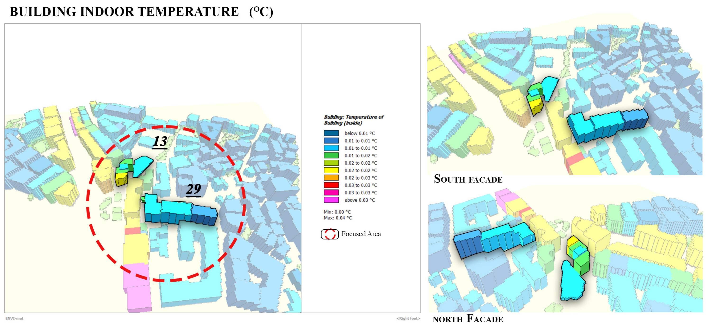
Finally, the analysis of the change in indoor temperature revealed a maximum increase of 0.04 °C when the stream line was uncovered (Figure 32). This change was mostly observed in the first row of buildings along the stream. For the buildings on the 13th and 29th blocks, a difference of 0.01 °C was observed at most, while no difference was measured for the other buildings (Figure 33).

5. Discussion

The literature aims to reduce the impact of urban heat islands on the thermal comfort of cities by analyzing parameters such as trees, green infrastructure, and urban morphology [3,5,6,8,9,11,12,13,19,34]. However, there is a lack of research analyzing the effect of green spaces and water surfaces on microclimatic conditions in winter cities. To the best of our knowledge, this research is among the first to analyze the microclimatic impacts of urban features in winter cities across two seasons and three different scales.

Within the scope of the analysis, the research focuses on the level of the impact of water surfaces on microclimate in built areas of cities with cold climates at three different levels, i.e., microclimate of building blocks, thermal comfort change, and temperature changes on the facades of buildings, which affect the heating and cooling loads of the buildings. The analysis and simulations were made during both the summer and winter periods in order to analyze the changing effects of water surfaces for different climate conditions.

The simulation results indicate that the uncovered water line led to a 16.9% reduction in air temperature and a 4.5% decrease in the thermal comfort index (PET) throughout the region during the summer season. Additionally, the results demonstrate a significant reduction in temperature stress in the area. During the winter period, the opening of the water channel resulted in a 0.44% increase in air temperature across the area. Simulations indicate that the most significant temperature difference occurs along the uncovered channel line, with an average width of 25 m. In this area, the air temperature can increase by up to 9.4%. The increase in temperature resulted in a 0.1% decrease in cold stress for thermal comfort. The low rate of thermal effect is likely due to the inability of the heated air to rise and be felt in this area. However, it is impossible to simulate the value change at the surface as ENVI-met automatically turns off the buoyancy term when the wind speed is below 0.8 m/s. As the wind speed in the case area is below 0.5 m/s in winter (Table 5), we need to explain this heat transfer effect through the natural convection dynamics without referring to buoyancy values. Natural convection is a process where fluid movement occurs due to buoyancy. Due to the low fluid velocity associated with natural convection, the heat transfer coefficient is also low. So, if the water surface remains colder than the air, the perceived heat flow is directed towards the water, which cools the air. Conversely, if the water surface is warmer than the air, the perceived heat flow is directed towards the air. Thermal effects are generally only relevant for people standing near water surfaces if they are perceived at a height of 1–2 m [55]. Therefore, it is believed that the hot air cannot rise significantly due to the air being below 0 degrees Celsius. Thus, the presence of water has a positive effect on both summer and winter temperatures in Erzurum.

The study also investigated the relationship between urban microclimate and energy exchange processes at the building level. Building indoor temperatures were evaluated by taking the average of the sampled buildings numbered 13 and 29 in the simulations. The results showed a decrease of 0.8 °C (3.5%) in indoor temperatures during the summer period due to the uncovering of the water channel. In contrast, a temperature increase of 0.01 °C (0.05%) was observed during the winter period. The changes in the indoor temperature values obtained in the simulations analyzing only the effect of water surfaces are very low. However, it should be considered that these values can increase much more when the whole area is planned and designed in accordance with the climate conditions. With urban design solutions such as buildings positioned according to the sun, green areas of appropriate size, and appropriate street orientations (southwest is the best in a cold climate), the temperature would increase even more. Therefore, although the analysis of microclimatic conditions gives low results, it can be concluded that they can have an impact on indoor temperature and energy consumption when considered together with climate-appropriate urban planning and design decisions.

This text examines the impact of current spatial interventions in Erzurum on urban climate and life, focusing on the Çaykara stream line as the study area. During the urban planning process, the Çaykara stream line was designated for a 20 m wide urban road by covering it, and this plan was implemented. However, this has resulted in negative microclimatic conditions in the current physical environment. This study identifies the concrete and positive effects of reintroducing the stream line. Today, similar practices continue in new growth areas in the city of Erzurum. Therefore, it can be concluded that current spatial interventions have a negative impact on the urban climate, leading to increased heat and cold stress. This study provides concrete evidence that water can increase temperatures in built-up areas of cities with winter conditions, while it has cooling effects in the same areas in summer conditions.

The study confirmed that changes in daily temperatures cause changes in electricity use, as previously emphasized in the literature. Additionally, the study found that energy exchange processes between the building facade and surrounding environments affect thermal performance at the building scale. The study demonstrates the interdependence of urban microclimate and building-level energy exchange processes. The results indicate that regulations based on microclimate can contribute to energy conservation and decrease the energy demand of the built sector.

In addition to reducing urban heat and lowering the average daily temperature in the dense city center, water surface treatment can also have a positive impact on microclimatic conditions during winter. This treatment can help reduce the cooling and heating loads of buildings.

6. Conclusions

This study presents a method for estimating microclimate changes resulting from the conversion of urban surfaces to water surfaces. It also quantitatively analyzes the resulting changes in building energy loads. The significance of this study, which distinguishes it from other literature, is that Erzurum is located on the northern slopes of the Palandöken Mountains at an altitude of 1853 m and experiences a winter period of more than 6 months. Furthermore, as heating loads are more significant than cooling loads in city buildings, the impact of outdoor temperature on building energy loads was determined by disregarding structural variations.

The simulations analyzed and evaluated the effects of summer and winter separately. The most significant finding is that water lines have a cooling effect in the summer (a decrease of 5 °C), while having an opposite effect in the winter, causing an increase in temperature (an increase of 0.02 °C). The simulation results indicate that the water line reduces the air temperature and thermal comfort index (from extreme heat stress to moderate heat stress) during the summer period, thereby reducing heat stress. During the winter period, it was found that there was an increase in air temperature. However, simulations indicate that this temperature difference is only effective up to certain distances (15 m—the first building facade line).

According to the simulations, the indoor temperature decreased slightly during the summer period (average 0.1–0.9 °C) when the water channel was uncovered and increased slightly during the winter period (max 0.04 °C). While the reductions in the heating and cooling loads of the buildings were minimal in this study, it is expected that a reduction in these energy loads can be achieved when the restoration of the Çaykara stream is applied to the entire surrounding area. Small savings in electricity costs can be achieved, particularly during the summer months for cooling.

Finally, the study emphasizes that even a small urban water body has positive consequences for Erzurum, and this should not be ignored by relevant policy-making institutions and organizations. Therefore, as the negative effects of water presence are increased in shaded areas, the policies should prioritize the precautions, focusing on minimizing them, in order to maximize the positive effects of water presence and, thus, the quality of life in cold cities.

The simulation results indicate that a high height/width ratio (shading effect) is advantageous by creating a shadow and cooling effect in the summer months but causes cold stress by decreasing PET values in the winter months. To avoid shadows on other buildings in winter and to maximize solar gain, it is recommended to propose wide streets and avenues. To ensure that water surfaces provide benefits throughout the year, it is important to carefully select their location within urban areas. Based on simulation results, it is more advantageous to use water in areas that receive ample solar access, particularly during the winter.