Enhancing Demand Prediction: A Multi-Task Learning Approach for Taxis and TNCs

Abstract

Taxis and Transportation Network Companies (TNCs) are important components of the urban transportation system. An accurate short-term forecast of passenger demand can help operators better allocate taxi or TNC services to achieve supply–demand balance in real time. As a result, drivers can improve the efficiency of passenger pick-ups, thereby reducing traffic congestion and contributing to the overall sustainability of the program. Previous research has proposed sophisticated machine learning and neural-network-based models to predict the short-term demand for taxi or TNC services. However, few of them jointly consider both modes, even though the short-term demand for taxis and TNCs is closely related. By enabling information sharing between the two modes, it is possible to reduce the prediction errors for both. To improve the prediction accuracy for both modes, this study proposes a multi-task learning (MTL) model that jointly predicts the short-term demand for taxis and TNCs. The model adopts a gating mechanism that selectively shares information between the two modes to avoid negative transfer. Additionally, the model captures the second-order spatial dependency of demand by applying a graph convolutional network. To test the effectiveness of the technique, this study uses taxi and TNC demand data from Manhattan, New York, as a case study. The prediction accuracy of single-task learning and multi-task learning models are compared, and the results show that the multi-task learning approach outperforms single-task learning and benchmark models.

1. Introduction

Taxi and Transportation Network Company (TNC) services play essential roles in the urban transportation system. Taxis offer traditional ride-hailing services, while TNCs such as Uber connect drivers and riders using Internet-based mobile technology. The ridership of TNCs has grown rapidly. For example, Uber’s ridership increased from 3.79 billion in 2017 to 6.3 billion in 2021 [1]. Thank to efficient driver–passenger matching technology and a more flexible pricing model, the capacity utilization rate of TNCs (the fraction of the time/mile in which a driver takes fare-paying passengers) is much higher than that of taxis [2]. Due to the popularity and innovative business model of TNCs, the ridership of taxis has lost ground in many cities. For example, in 2016, the number of TNC trips made was 12 times that of taxi trips in San Francisco [3].

Improving short-term demand forecasting for both TNCs and taxis has positive impacts on sustainability. With accurate prediction, operators can assign the right number of vehicles at the right time to reduce the idle time of drivers and waiting time for passengers, leading to an improved capacity utilization ratio. The capacity utilization ratio is seldom revealed by TNCs or taxi companies, but a study has shown its value ranged between 43.5% and 51.7% for selected cities in the United States between 2013 and 2015 [2]. Improving the utilization ratio could potentially help address traffic congestion problems, improve traffic speeds, and reduce traffic emissions.

Various studies have developed short-term demand forecasting models for transportation modes. Some studies have used traditional time-series forecasting models such as autoregressive integrated moving average (ARIMA) and its variants to predict traffic demand [4,5,6] by capturing the temporal correlation of data. Recently, with the advent of a higher computing power and the popularization of AI technologies, many studies have applied neural network models to demand forecasting [7,8,9].

The majority of studies mentioned earlier are based on single-task learning, where the model predicts for one transportation mode only. Recently, multi-task learning (MTL) has garnered significant attention in the AI domain, as it enables different tasks to share information, thereby enhancing the prediction accuracy. Some transportation demand forecasting research has also adopted this technique [10,11,12,13,14]. However, the majority of these studies allow information sharing between tasks without controlling for “negative transfer”, which is common and could reduce the effectiveness of multi-task learning.

The demand patterns for TNCs and taxis are closely correlated. For example, in New York City, TNCs and taxis show similar spatial–temporal patterns [15,16], and their demand is correlated with the same set of land use and sociodemographic factors [17]. Given such correlated patterns, leveraging information sharing between the two modes could potentially improve the demand forecasting accuracy. The idea of incorporating TNC information into a taxi demand forecasting model has been experimented with, which showed an improvement in the model prediction accuracy [15]. However, this study did not embed taxi information into a TNC model, and there have been no studies developing a multi-task learning model to simultaneously predict the demand for these two modes. In New York City, Yellow Cabs can be hailed on the Uber app [18], a partnership that provides an opportunity for data sharing and modeling, which could potentially improve the demand forecasting accuracy for both the taxi and TNC modes.

To capture the spatial dependency of demand, previous studies utilized first-order relationships to construct spatial graphs, such as considering the distance between two zones [19,20] or determining whether two zones are neighbors [21]. These researchers commonly assume that zones closer to each other or in proximity have a stronger relationship. This research explores a higher order of spatial dependency, which could capture more comprehensively the interaction of spatial relationships, which has not been explored in the literature yet.

To fill in the research gaps, this study proposes a multi-task learning approach to forecast the demand for taxis and TNCs simultaneously. The model adopts a gating mechanism that selectively shares information between the two modes to avoid the negative transfer that commonly occurs in MTL. In addition, the model also captures the second-order spatial dependency of the demand by applying a graph convolutional network. The contribution of this study is threefold:

• The evolving shared mobility sector longs for better demand prediction for different formats of sharing services. This study proposes a multi-task learning model to predict the demand for the TNC and taxi modes simultaneously to meet these needs.
• This study explores methodological improvements to increase the prediction accuracy. The techniques considered include a gating mechanism to mitigate the negative transfer between the two modes and spatial embedding, capturing the interaction of spatial dependency.
• Extensive experiments are conducted using actual taxi and TNC trip data from Manhattan, NYC. The experimental results show that the proposed modeling approach outperforms the single-task learning model and other benchmark learning models.

2. Literature Review

This section reviews the research-related methods for capturing spatiotemporal dependency and multi-task learning.

2.1. Modeling Spatial–Temporal Dependency of Transportation Demand

Utilizing telematics technology, taxi companies can collect detailed data for each trip, including pick-up/drop-off zones, start/end time, and trip trajectories. This produces a vast amount of data, which has attracted significant research interest. Researchers have explored the data in various ways, including analyzing spatial–temporal demand patterns [22,23,24], exploring the impact of urban structures (e.g., land use patterns, access to different transportation modes, etc.) on taxi demand [25,26], building short-term demand forecasting models [27,28], and developing models for the visual querying of taxi trip data [29]. These efforts help us understand travel behaviors and support evidence-based policymaking.

To conduct short-term demand forecasting, capturing the spatial–temporal correlation is essential. For a neural-network-based forecasting model, a common approach is to stack spatial layers and temporal layers in the models, and this approach has been adopted in [7,30].

Modeling spatial dependency can improve the prediction accuracy [21,31,32]. There are generally two techniques used to capture the spatial dependency of zones: convolutional neural networks (CNNs) and graph neural networks (GNNs). The first approach requires the study area to be partitioned into regular grids, such as image pixels, and the demand of a zone is analogous to the value of a pixel in an image [7]. The second approach can handle non-Euclidean structural data such as friendship networks, transportation networks, etc. Due to their flexibility and potentially better performance, graph neural networks [33,34] have become more popular in recent years. To construct a graph of a transportation network, nodes are defined as zonal areas, and edges are defined in various ways depending on the specific definition. Edges can be defined based on whether two zones have traffic flow [31], whether two zones are spatial neighbors, whether zones are connected by major roads or have similar POIs [21], the distance between nodes [19,35], etc. However, in the existing literature, the aforementioned definitions are limited to first-order spatial dependency.

To capture the temporal dependency of transportation demand, popular techniques include Long Short-Term Memory (LSTM) [36] and Gated Recurrent Units (GRUs) [9]. Compared to LSTM, GRUs have a lighter computing burden and still achieve comparable performance. Historical time steps might contribute differently to the forecasting of the next time stamp. Hence, the attention method could be applied to extract historical time steps that are important to demand. The attention mechanism has been shown to be effective in improving the demand forecasting accuracy [9,21,37,38].

2.2. Multi-Task Learning

MTL involves learning multiple related tasks simultaneously to improve the generalization performance of the forecasting model. In the transportation demand forecasting domain, the application of MTL is thriving. Some studies have applied MTL to predicting different tasks for one transportation mode. A task includes predicting the demand in a zone [27,39] or predicting pick-up/drop-off [28], etc. Though these studies show the benefits of MTL in improving the prediction accuracy, they simply share information between tasks without differentiating between positive and negative information. There were also a few studies we found that applied MTL to predicting the demand for multiple transportation modes. For example, one study developed a knowledge adaptation module that boosted the prediction of transportation modes with fewer stations (e.g., ferries) by adapting the demand pattern from station-intensive modes (e.g., buses). The model results show that MTL improves the demand forecasting performance for modes with fewer stations [10]. Another study we found looked into demand prediction for the subway and TNCs [40].

In an MTL model, sharing parameters between tasks is not always successful; if shared tasks are not closely related or information is shared too extensively, this can affect the model performance. This phenomenon is called “negative transfer” and is common in applications such as natural language processing [41] and computer vision [42]. To reduce the negative influence of task sharing, some MTL studies have attempted to answer questions on which layers to share, what parameters to share, how to address implicit or explicit task relationships, and how to define the importance of tasks [41,42,43]. These MTL approaches share full or partial features between tasks without discerning their helpfulness, while gated MTL [44] adopts a gating mechanism called a Gated Sharing Unit that can filter the feature flows between tasks and greatly reduce task inference.

3. Methodology

This section defines the problem of demand forecasting for taxis and TNCs, introduces a single-task learning model that can be used for predicting taxi or TNC demand, and also describes the gating mechanism that is used to build the multi-task learning model.

3.1. Preliminary: Problem Definition

The demand forecasting problem aims to predict the demand for multiple transportation modes M for the study areas A at the time interval t + 1 given historical demands until time interval t, where A = {a₁, a₂, …, a_n} is denoted as the set of areas; M = {m₁, m₂, … m_j} is the set of transportation modes; the set of time sequences is denoted as I = {1, 2 …, t, …, T}; and the historical time sequence can be defined as ${\mathit{l}}_t=\{t-k, t-k+1, \dots , t\}$, where k is a recall factor. Mathematically, the problem can be defined as

$${\mathit{y}}_{t+1}^{\mathit{A},\mathit{M}}=F({\mathit{y}}_{t-k}^{\mathit{A},M}, \dots {\mathit{y}}_t^{\mathit{A},M})$$

(1)

where ${\mathit{y}}_{t+1}^{\mathit{A},\mathit{M}}$ is the transportation demand for areas A and modes M at t + 1, and F(∙) is the forecasting function with inputs on historical passenger demand for the transportation modes. The following section firstly describes the single-task learning model, and then introduces the MTL model that is built based on the single-task learning model.

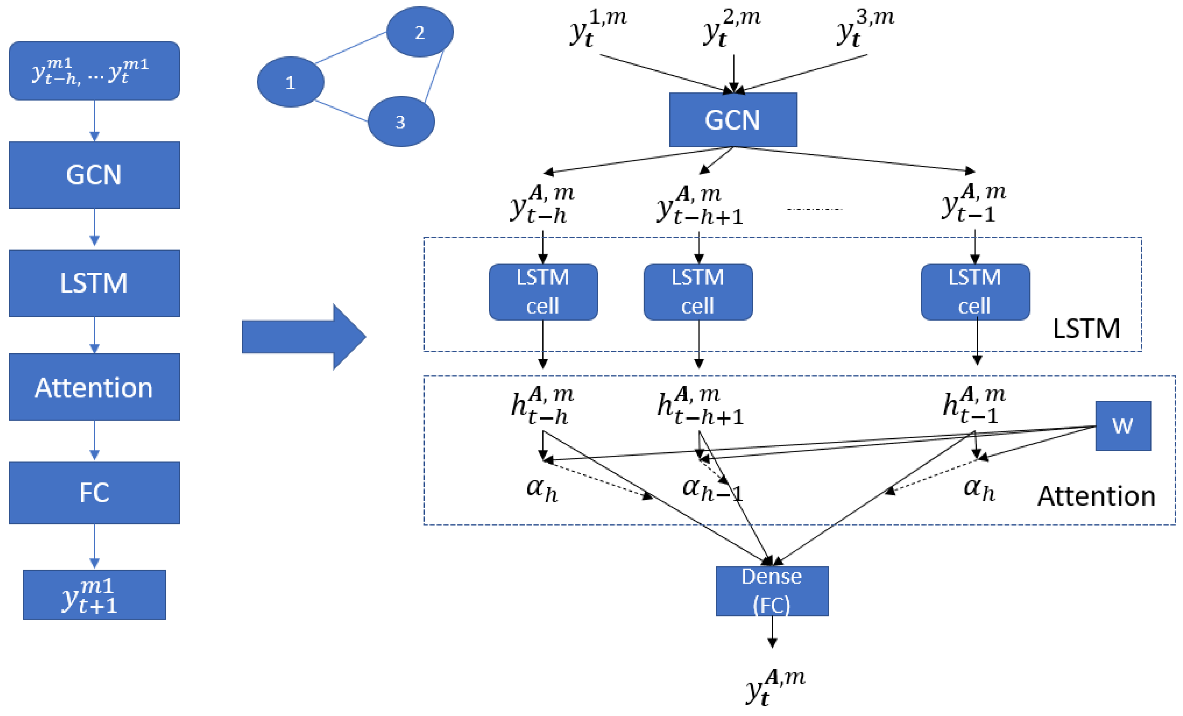
3.2. Single-Task Learning Model

A single-task learning model stacks GCN and LSTM layers and incorporates an attention layer to enhance the forecasting accuracy. The model is designed to capture the spatial–temporal dependency of transportation demand and is composed of six layers, as shown in Figure 1.

The first layer is an input layer, with the input being the historical demand for taxis or TNCs. The input is then passed to the GCN layer to capture the spatial dependency, and its output is then passed to LSTM to capture the temporal dependency. The fourth layer is an attention layer, which assigns different weights to the output from LSTM. Higher weights are assigned to the outputs that are more correlated with our prediction. The fifth layer is a fully connected layer, and the last layer is an output layer. Next, we will explain each layer in more detail.

Input Layer: The input layer is the input for the model. It is the historical demand for taxis or TNCs for different zones.

Graph Convolutional Layer: In the context of transportation, a network can be depicted as a graph, with nodes representing various entities like taxi zones, communities, neighborhoods, traffic analysis zones, or census tracts and edges indicating relationships between nodes (e.g., neighboring taxi zones). The signal of a node refers to the historical demand from its corresponding zone. A graph convolutional network (GCN) [34] works by smoothing a node’s signal through the transformation and aggregation of the demand data from its neighboring nodes (e.g., nearby taxi zones). The graph convolutional layer is defined as

$$\mathit{Z}=\tilde{\mathit{A}}\mathit{X}\mathit{W}$$

(2)

where $\mathit{Z}\in {\mathit{R}}^{N\times D}$ is the output from the GCN, $\tilde{\mathit{A}}\in {\mathit{R}}^{N\times N}$ is the normalized adjacency matrix with self-loops, $\mathit{X}\in {\mathit{R}}^{N\times K}$ is the input for the GCN, and $\mathit{W}\in {\mathit{R}}^{K\times D}$ is the learned weight. A GCN structure is adopted in this study to capture the spatial dependency between zones.

Long Short-Term Memory Layer: LSTM is adopted in this study to capture temporal dependency. LSTM has been popularly used in demand forecasting research, such as the studies [27,32]. An LSTM cell has the structure shown in Figure 2. Each cell has inputs of ${\mathit{x}}_t$, a hidden state ${\mathit{h}}_{t-1}$, and a cell state ${\mathit{c}}_{t-1}$ and outputs the hidden state ${\mathit{h}}_t$ as the final output or as the input to the next cell and ${\mathit{c}}_t$ to the next cell state. The structure within the cell has the ability to decide what information to store or throw away for cell state c; it continues to update based on different time steps and finally decides the output. A detailed explanation of LSTM is provided in [45]. The formulation for the computation in an LSTM cell is shown in Figure 2 and explained thereafter.

$$\mathit{f}=\sigma \left({\mathit{w}}_f·\left[{\mathit{h}}_{t-1},{\mathit{x}}_t\right]+{\mathit{b}}_f\right)$$

(3)

$$\mathit{i}=\sigma \left({\mathit{w}}_i·\left[{\mathit{h}}_{t-1},{\mathit{x}}_t\right]+{\mathit{b}}_i\right)$$

(4)

$$\mathit{g}=tanh({\mathit{w}}_g·\left[{\mathit{h}}_{t-1},{\mathit{x}}_t\right]+{\mathit{b}}_g)$$

(5)

$$\mathit{o}=\sigma \left({\mathit{w}}_o·\left[{\mathit{h}}_{t-1},{\mathit{x}}_t\right]+{\mathit{b}}_o\right)$$

(6)

$${\mathit{c}}_t=\mathit{f}⨀{\mathit{c}}_{t-1}+\mathit{i}⨀\mathit{g}$$

(7)

$${\mathit{h}}_t=\mathit{o} ⨀ \mathrm{t}\mathrm{a}\mathrm{n}\mathrm{h}\left({\mathit{c}}_t\right)$$

(8)

where $\sigma$ is a sigmoid function that is given by $\sigma \left(x\right)=\frac{1}{1+e^x}$. It outputs values between 0 and 1, which controls the flow of information. The cross symbol in the figure refers to multiplication, and the plus symbol is a merge function that outputs the sum of the inputs.$⨀$ is elementwise multiplication. ${\mathit{w}}_f$, ${\mathit{w}}_g$, ${\mathit{w}}_i$, ${\mathit{w}}_o$, ${\mathit{b}}_f$, ${\mathit{b}}_g$, ${\mathit{b}}_i$, and ${\mathit{b}}_o$ are trainable parameters.

Attention Layer: The attention mechanism applied in this study is from Yang et al. [46], which had success in dealing with sequence learning tasks. Mathematically, the attention method is defined as:

$${\mathit{u}}_i=\tanh \left({\mathit{W}}_w{\mathit{h}}_i+{\mathit{b}}_w\right)$$

(9)

$${\mathit{\alpha }}_i=\frac{\exp \left({{\mathit{u}}_i}^T{\mathit{u}}_w\right)}{\sum _{i\in l_t}\exp \left({{\mathit{u}}_i}^T{\mathit{u}}_w\right)}$$

(10)

$$\widetilde{{\mathit{h}}_t}=\sum _{i\in l_t}{\mathit{\alpha }}_i{\mathit{h}}_i$$

(11)

where the hidden output ${\mathit{h}}_i=\{h_{t-k}, \dots h_t\}$ is fed into Equation (9) to obtain ${\mathit{u}}_i$ as the hidden representation of ${\mathit{h}}_i$. Then, the importance of the time step (t − k) is measured as the similarity between ${\mathit{u}}_i$ and ${\mathit{u}}_w$, which is normalized to ${\mathit{\alpha }}_i$ using a softmax function. Finally, the output $\widetilde{{\mathit{h}}_t}$ is the weighted sum of the hidden representation of ${\mathit{h}}_i$. ${\mathit{u}}_w$ in Equation (10) functions as the high-level representation of the “important time step”. During training, ${\mathit{u}}_w$, ${\mathit{W}}_w$, and ${\mathit{b}}_w$ are randomly initialized and jointly learned in the model.

Fully Connected Layer: FC refers to the fully connected layer or dense layer in a neural network. This layer has the number of neurons that is equal to the number of zones for forecasting. The neurons are connected to every neuron in the preceding layer.

Output Layer: The output layer generates the future demand (e.g., next hour) of different zones.

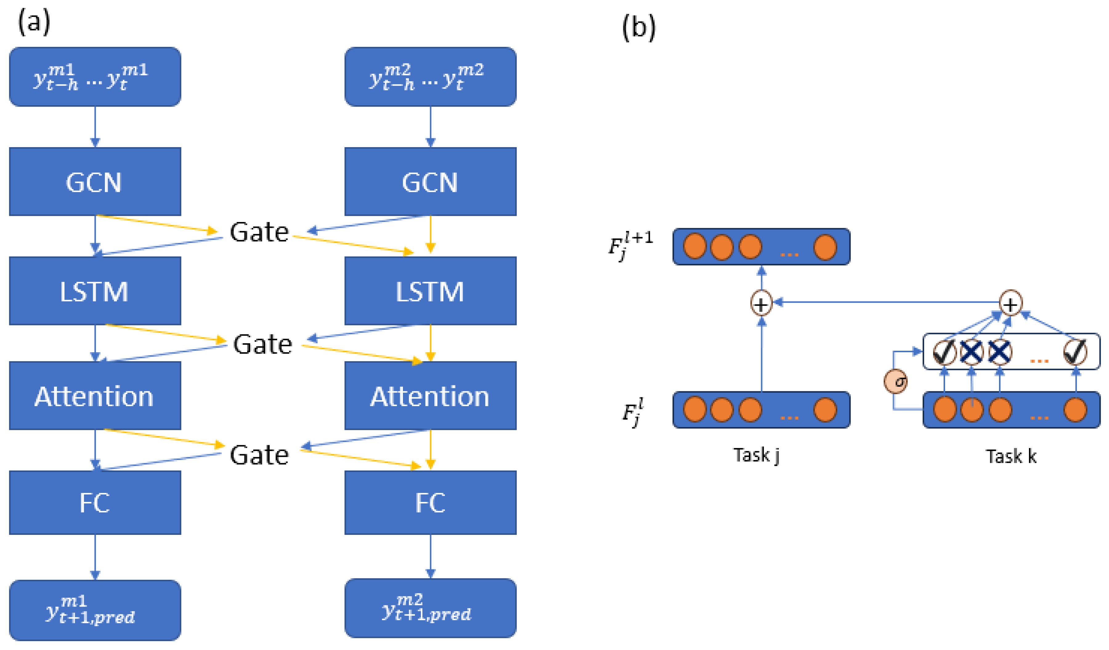
3.3. Multi-Task Learning Model

To build a multi-task learning model, this study adopts a “gating” mechanism called a Gated Sharing Unit (GSU) [44] as shown in Figure 3b. A GSU allows the model to filter features from other tasks and select those that are useful to the task; it avoids harmful feature inference if two feature maps are concatenated directly. The overall architecture of the model is depicted in Figure 3a.

There are two steps involving a GSU. Assume that there are two modes, j and k. The first step computes how much information will be merged from mode k to mode j. For this purpose, a gate is inserted to select the useful features from mode k, which is calculated using

$${\mathit{g}}_{jk}^l=\sigma ({\mathit{W}}_{jk}^l·{\mathit{F}}_k^l+{\mathit{b}}_{jk}^l)$$

(12)

where l is the level of the layers, and σ is a sigmoid function that guarantees the values of g are bounded between 0 and 1. ${\mathit{W}}_{jk}^l$ is the weight that will be trained, ${\mathit{F}}_k^l$ are the output parameters of mode k in layer l, and ${\mathit{b}}_{jk}^l$ is the bias term. ${\mathit{g}}_{jk}^l$ is a vector. The gate controls how much information from mode k at layer l will be passed to mode j. As shown in Figure 3b, the check mark indicates that more information from the preceding neuro will contribute to task j, while the cross mark indicates less information contribution.

The second step computes the merge of features between mode j and mode k. It can be calculated using the following equation:

$${\mathit{F}}_j^{l+1}=\sum _{ k\ne j}{\mathit{g}}_{jk}^l \odot {\mathit{F}}_k^l+{\mathit{F}}_j^l$$

(13)

where $\odot$ denotes elementwise multiplication. This formula outputs the fused parameters ${\mathit{F}}_j^{l+1}$. From this equation, the features from mode j are directly passed to the next layer, and the features from mode k are merged into mode j after filtering using the gate ${\mathit{g}}_{jk}^l$.

4. Experiments and Model Performance Evaluation

This section describes the experiment settings and presents a performance evaluation of the proposed models.

4.1. Study Area

4.1.1. Study Site Selection and Data Preprocessing

This study selected Manhattan, New York, as the case study area, as both Yellow Cabs and TNCs service that area, and trip data are publicly accessible from the NYC Taxi & Limousine Commission [47]. One-year trip data for 2018 are retrieved for the study, including Yellow Cab and For-Hire Vehicle (FHV) trip data. The FHV data includes Uber, Lyft, and other platforms that allow passengers to use apps to request trip services.

For both transportation modes, information such as trip pick-up zone, drop-off zone, pick-up time, and drop-off time is selected from the dataset. To remove erroneous trip records, trips are filtered according to travel time and travel distance. The minimum travel time duration is set to 1 min, with the maximum set to 2 h and the minimum travel distance set to be greater than 0.2 miles. This results in a dataset containing 87.1 million records of taxi trips and 99.3 million records of TNC trips within Manhattan. The trip data are aggregated at the hourly level, with each zone representing the hourly demand for taxi and TNC services. In total, the processed dataset comprises 59 taxi zones (features) and 8760 time steps (365 days × 24 h per day).

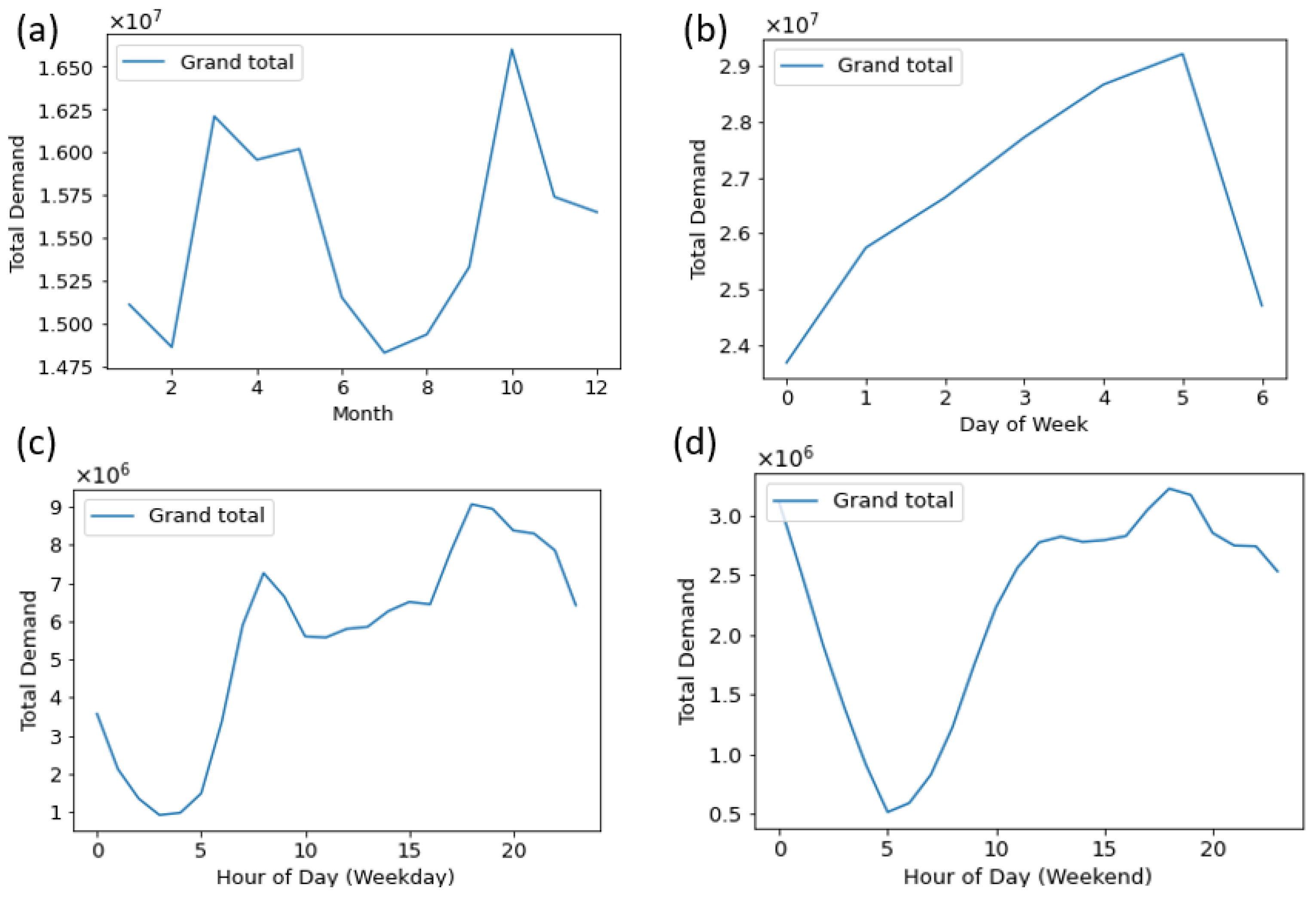
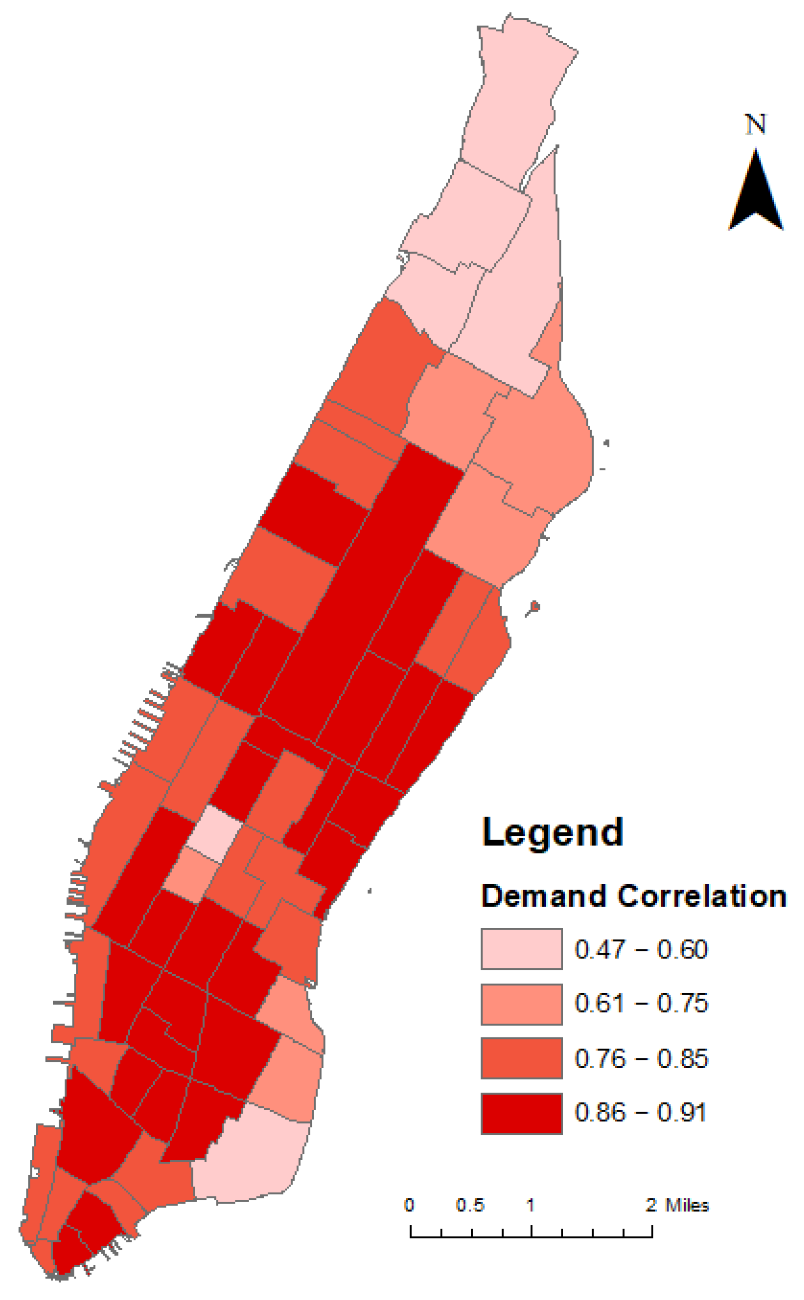
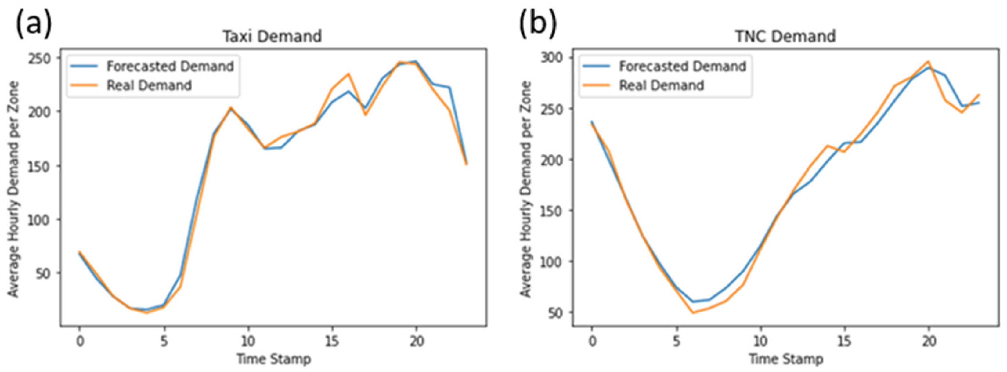
4.1.2. Data Analysis

Figure 4 illustrates the aggregated monthly, daily, and hourly trips for taxi and TNC services, while Figure 5 shows the total trip counts for both transportation modes. The correlation coefficient in Figure 4 is calculated using Pearson’s correlation method. As depicted in Figure 4a, there is an inverse relationship between taxi and TNC demand on a monthly basis—TNC demand displays a rising trend while taxi demand declines. This suggests a competitive dynamic between TNC and taxi services in the Manhattan area. At the aggregate trip level (Figure 5a), a seasonal pattern emerges, with both taxi and TNC trips peaking in popularity during October and March and decreasing during the summer and winter months. The daily (Figure 4b) and hourly (Figure 4c,d) patterns reveal a similar temporal demand pattern for both TNC and taxi services, as indicated by the positive correlation coefficient. The similarity in demand patterns is also evident in the total demand analysis (Figure 5b–d). The strong correlation between the two modes suggests MTL is a suitable approach to jointly modeling taxi and TNC demand. Examining Figure 4c,d, it is observed that the TNC demand generally tends to be slightly higher, with both modes following a comparable hourly trend. However, there are instances where the taxi demand equals or exceeds the TNC demand at certain hours, indicating temporal volatility at a finer granularity. This volatility may introduce noise into the MTL approach if information sharing between the modes is simply uniform. Therefore, it is crucial for the MTL model to selectively filter unnecessary information for effective information exchange.

The above analysis is conducted for all study areas. A similar hourly pattern is also identified at the local level, as shown in Figure 6. The correlation coefficient is computed for each taxi zone at the hourly level and is positive for all zones, as shown in Figure 5, which suggests the close short-term demand correlation between taxis and TNCs. Thus, sharing the information between the two modes could potentially be beneficial to the model.

4.2. Model Training

The 2018 one-year dataset included 8760 time steps, with the data arranged sequentially by time. The first 85% (approximately 310 days) is used for training, and the remaining 15% is used for testing. The “looking back” time step is set as 12, which means 12 h historical demand is used to forecast the demand for the next time step (next hour).

The constructed model has four layers: the GCN, LSTM, attention, and dense layers (as illustrated in Figure 1 and Figure 3). TensorFlow 2.1 [48], an open-source library renowned for training neural network models, is utilized for training the model. Training stops after the training loss is higher than the minimum training loss for five consecutive epochs. The model is implemented using the Python programming language, and the hardware used for model training includes an Intel(R) Core(TM) i7-9750H CPU with 16 GB of RAM.

4.3. Model Evaluation

4.3.1. Description of the Baseline Models and the Proposed Models in the Experiment

To demonstrate the performance of the proposed MTL model, besides the single-task learning model, several popular time-series models are also selected for comparison. The baseline models include the following:

• ARIMA: An autoregressive integrated moving average model, a statistical model widely used for time-series forecasting.
• MLP: A multi-layer perception, the most basic neural network. In this study, a three-layer neural network is used, which includes an input layer, a dense layer, and an output layer.
• XGBoost: eXtreme Gradient Boosting, which applies boosting to a tree-based machine learning model—widely known as an efficient model that solves data science problems accurately [49].

To test the effectiveness of MTL and the interaction of spatial dependency, we also compare models that do not consider spatial dependency, considering first-order spatial dependency, and considering the interaction of spatial dependency. Each variation of single-task learning and MTL is built. Specifically, we have the models listed as below:

• Single-task learning (without a GCN): Single-task learning model shown in Figure 1 without a GCN layer.
• Multi-task learning (without a GCN): MTL model shown in Figure 3 without a GCN layer. The Gated Sharing Unit is applied after the LSTM layer.
• Single-task learning (GCN-Distance): Single-task learning model shown in Figure 1, with graph edge defined as the inverse distance between zones.
• Multi-task learning (GCN-Distance): MTL model shown in Figure 3, with graph edge defined as the inverse distance between zones.
• Single task learning (GCN-Neighbor): Single-task learning model shown in Figure 1, with graph edge defined as 1 if two zones share boundaries and 0 otherwise.
• Multi-task learning (GCN-Neighbor): MTL model shown in Figure 3, with graph edge defined as 1 if two zones share boundaries and 0 otherwise.
• Single task learning (GCN-Interaction): Single-task learning model shown in Figure 1, with graph edge defined as the product of inverse distance dependency and neighbor dependency.
• Multi-task learning (GCN-Interaction): MTL model shown in Figure 3, with graph edge defined as the product of inverse distance dependency and neighbor dependency.

4.3.2. Evaluation Metrics

To compare the performance of these models, this study adopted two metrics which are popularly used for regression tasks—the Mean Absolute Error (MAE) and Root Mean Squared Error (RMSE)—given by

$$MAE=\frac{1}{n}{\sum }_{i=1}^n\left|y_i-\widehat{y_i}\right|$$

(14)

$$RMSE=\sqrt{\frac{1}{n}{\sum }_{i=1}^n{(y_i-\widehat{y_i})}^2}$$

(15)

where $y_i$ is the ground truth value and $\widehat{y_i}$ is the predicted value.

4.4. Results and Discussions

This section compares the performance of the baseline models and the proposed models.

Table 1. Model performance comparison among different methods.

	Taxi		TNC
	RMSE	MAE	RMSE	MAE
ARIMA	54.1	32.6	56.3	37.1
MLP	47.9	30.0	49.5	34.4
XGBoost	36.9	21.8	41.0	26.1
Single-task learning (without a GCN)	37.7	22.6	41.0	27.2
Multi-task learning (without a GCN)	36.1	21.8	39.5	26.1
Single-task learning (GCN-Distance)	36.7	21.8	40.2	26.2
Multi-task learning (GCN-Distance)	35.8	21.5	40.5	25.9
Single-task learning (GCN-Neighbor)	37.4	22.2	39.8	26.1
Multi-task learning (GCN-Neighbor)	36.5	21.9	39.4	25.5
Single-task learning (GCN-Interaction)	35.8	21.1	38.2	25.0
Multi-task learning (GCN-Interaction)	34.7	20.9	37.2	24.2

shows the results of the evaluation metrics for the different models. Overall, the proposed models have a better performance compared to the baseline models, the MTL models beat the single-task learning models, and considering spatial interactions brings additional benefits. Looking into the details of the model evaluation, it is interesting to see that the XGBoost model has an RMSE of 36.9 and an MAE of 21.8 for the taxi mode, which is slightly better than the single-task learning model without a GCN, suggesting that the XGBoost model, in this case, performs very well for time-series forecasting. When a gating unit is applied (MTL), the multi-task learning model without a GCN performs better than the single-task learning model without a GCN and XGBoost, suggesting the effectiveness of parameter sharing in MTL. Table 1 also shows the model performance when the distance dependency or neighbor dependency is considered, and their prediction accuracy outperforms the models that do not consider a GCN. When the distance dependency is captured, the taxi prediction errors are lower than those for the model capturing neighbor dependency, but the model’s TNC prediction errors are a bit higher. Finally, we also test the model that considers the interaction between distance dependency and neighbor dependency. As Table 1 shows, the model performance further improves, and, again, the MTL model outperforms the single-task learning model, which makes MTL (GCN-Interaction) the best model.

To visualize the model’s performance, a random sample of the predicted and actual demand for one day (24 time stamps) from the test data was taken. Figure 7a shows the forecasted demand and real demand for taxis averaged across all zones, with a similar representation for TNCs shown in Figure 7b. Both figures reveal a close match between the forecasted and observed demand, indicating the good performance of the model.

5. Conclusions

This study develops a multi-task learning model for predicting the short-term demand of taxis and TNCs. The study selects Manhattan as the case study area and explores the short-term and long-term demand correlation for taxis and TNCs. At the short-term (hourly) level, the demand for taxis and TNCs presents similar patterns, which indicates it could be beneficial to share information between the two modes in a model. The developed multi-task learning model employs a gating mechanism that selectively shares information across the two modes. The experimental results and a model performance comparison show that MTL outperforms single-task learning and other baseline models. This study also investigates the spatial dependency of the demand model, and considering the interaction of spatial dependency outperforms the first-order dependency that is commonly used in the literature.

Given the effectiveness of the methodology, TNC companies can leverage this technique to enhance their forecasting accuracy, leading to various improvements in resource allocation efficiency. For example, by accurately predicting spikes in demand within specific areas, TNC companies can strategically deploy TNC or taxi drivers to minimize the wait time for passengers. Additionally, short-term demand forecasting also facilitates the anticipation of traffic congestion in particular areas, enabling TNCs to optimize their routes. From a traffic management standpoint, integrating predictions of demand for taxi and TNC services into existing intelligence transportation systems can effectively contribute to reducing traffic congestion and enhancing the reliability of transportation options.

Several potential research directions could be extended from this study. First, while this study applies effective MTL techniques, it would be worthwhile to explore other advanced MTL techniques, such as gradient surgery [50], to test whether the prediction errors can be further reduced. A summary of the MTL literature is available in [51]. Second, some transportation modes may exhibit weaker correlations but still have significant implications, such as shared e-scooters and TNCs, which have a competing relationship [52]. Investigating whether MTL can effectively model these modes would be an interesting avenue of research. Third, the GSU technique could be tested with data from different cities or for different tasks (e.g., traffic flow, TNC/taxi forecasting) to demonstrate its generalizability. Fourth, while improved demand forecasting can benefit route planning, the impact of this forecasting on traffic congestion remains a question worth exploring.

References

1. Iqbal, M. Uber Revenue and Usage Statistics. Available online: https://www.businessofapps.com/data/uber-statistics/ (accessed on 28 March 2023).
2. Cramer, J.; Krueger, A.B. Disruptive change in the taxi business: The case of Uber. Am. Econ. Rev. 2016, 106, 177–182. [Google Scholar] [CrossRef]
3. SFCTA. TNCs Today: A Profile of San Francisco Transportation Network Company Activity; SFCTA: San Francisco, CA, USA, 2017.
4. Shekhar, S.; Williams, B.M. Adaptive seasonal time series models for forecasting short-term traffic flow. Transp. Res. Rec. 2007, 2024, 116–125. [Google Scholar] [CrossRef]
5. Li, X.; Pan, G.; Wu, Z.; Qi, G.; Li, S.; Zhang, D.; Zhang, W.; Wang, Z. Prediction of urban human mobility using large-scale taxi traces and its applications. Front. Comput. Sci. 2012, 6, 111–121. [Google Scholar] [CrossRef]
6. Moreira-Matias, L.; Gama, J.; Ferreira, M.; Mendes-Moreira, J.; Damas, L. Predicting taxi–passenger demand using streaming data. IEEE Trans. Intell. Transp. Syst. 2013, 14, 1393–1402. [Google Scholar] [CrossRef]
7. Ke, J.; Zheng, H.; Yang, H.; Chen, X.M. Short-term forecasting of passenger demand under on-demand ride services: A spatio-temporal deep learning approach. Transp. Res. Part C Emerg. Technol. 2017, 85, 591–608. [Google Scholar] [CrossRef]
8. Yao, H.; Tang, X.; Wei, H.; Zheng, G.; Li, Z. Revisiting spatial-temporal similarity: A deep learning framework for traffic prediction. In Proceedings of the AAAI Conference on Artificial Intelligence, Honolulu, HI, USA, 27 January–1 February 2019; pp. 5668–5675. [Google Scholar]
9. Jin, G.; Cui, Y.; Zeng, L.; Tang, H.; Feng, Y.; Huang, J. Urban ride-hailing demand prediction with multiple spatio-temporal information fusion network. Transp. Res. Part C Emerg. Technol. 2020, 117, 102665. [Google Scholar] [CrossRef]
10. Li, C.; Bai, L.; Liu, W.; Yao, L.; Waller, S.T. Knowledge adaption for demand prediction based on multi-task memory neural network. In Proceedings of the 29th ACM International Conference on Information & Knowledge Management, Online, 19–23 October 2020; pp. 715–724. [Google Scholar]
11. Bai, L.; Yao, L.; Kanhere, S.S.; Yang, Z.; Chu, J.; Wang, X. Passenger demand forecasting with multi-task convolutional recurrent neural networks. In Proceedings of the Pacific-Asia Conference on Knowledge Discovery and Data Mining, Macau, China, 14–17 April 2019; pp. 29–42. [Google Scholar]
12. Ke, J.; Feng, S.; Zhu, Z.; Yang, H.; Ye, J. Joint predictions of multi-modal ride-hailing demands: A deep multi-task multi-graph learning-based approach. Transp. Res. Part C Emerg. Technol. 2021, 127, 103063. [Google Scholar] [CrossRef]
13. Liang, J.; Tang, J.; Gao, F.; Wang, Z.; Huang, H. On region-level travel demand forecasting using multi-task adaptive graph attention network. Inf. Sci. 2023, 622, 161–177. [Google Scholar] [CrossRef]
14. Liu, H.; Wu, Q.; Zhuang, F.; Lu, X.; Dou, D.; Xiong, H. Community-Aware Multi-Task Transportation Demand Prediction. In Proceedings of the AAAI Conference on Artificial Intelligence, Online, 2–9 February 2021. [Google Scholar]
15. Zhao, J.; Chen, C.; Huang, H.; Xiang, C. Unifying Uber and taxi data via deep models for taxi passenger demand prediction. Pers. Ubiquitous Comput. 2020, 27, 523–535. [Google Scholar] [CrossRef]
16. Poulsen, L.K.; Dekkers, D.; Wagenaar, N.; Snijders, W.; Lewinsky, B.; Mukkamala, R.R.; Vatrapu, R. Green cabs vs. uber in new york city. In Proceedings of the 2016 IEEE International Congress on Big Data (BigData Congress), San Francisco, CA, USA, 27 June–2 July 2016; IEEE: Piscataway, NJ, USA, 2016; pp. 222–229. [Google Scholar]
17. Correa, D.; Xie, K.; Ozbay, K. Exploring the taxi and Uber demand in New York City: An empirical analysis and spatial modeling. In Proceedings of the 96th Annual Meeting of the Transportation Research Board, Washington, DC, USA, 8–12 January 2017. [Google Scholar]
18. Hu, W.; Browning, K.; Zraick, K. Uber Partners with Yellow Taxi Companies in N.Y.C. Available online: https://www.nytimes.com/2022/03/24/business/uber-new-york-taxis.html (accessed on 30 March 2023).
19. Li, Y.; Yu, R.; Shahabi, C.; Liu, Y. Diffusion convolutional recurrent neural network: Data-driven traffic forecasting. arXiv 2017, arXiv:1707.01926. [Google Scholar]
20. Yu, X.; Shi, S.; Xu, L. A spatial–temporal graph attention network approach for air temperature forecasting. Appl. Soft Comput. 2021, 113, 107888. [Google Scholar] [CrossRef]
21. Geng, X.; Li, Y.; Wang, L.; Zhang, L.; Yang, Q.; Ye, J.; Liu, Y. Spatiotemporal multi-graph convolution network for ride-hailing demand forecasting. In Proceedings of the AAAI Conference on Artificial Intelligence, Honolulu, HI, USA, 27 January–1 February 2019; pp. 3656–3663. [Google Scholar]
22. Bischoff, J.; Maciejewski, M.; Sohr, A. Analysis of Berlin’s taxi services by exploring GPS traces. In Proceedings of the 2015 International Conference on Models and Technologies for Intelligent Transportation Systems (MT-ITS), Budapest, Hungary, 3–5 June 2015; pp. 209–215. [Google Scholar]
23. Nuzzolo, A.; Comi, A.; Papa, E.; Polimeni, A. Understanding taxi travel demand patterns through Floating Car Data. In Proceedings of the Conference on Sustainable Urban Mobility, Skiathos Island, Greece, 24–25 May 2018; Springer: Cham, Switzerland, 2018; pp. 445–452. [Google Scholar]
24. Dong, X.; Zhang, M.; Zhang, S.; Shen, X.; Hu, B. The analysis of urban taxi operation efficiency based on GPS trajectory big data. Phys. A Stat. Mech. Its Appl. 2019, 528, 121456. [Google Scholar] [CrossRef]
25. Yang, Z.; Franz, M.L.; Zhu, S.; Mahmoudi, J.; Nasri, A.; Zhang, L. Analysis of Washington, DC taxi demand using GPS and land-use data. J. Transp. Geogr. 2018, 66, 35–44. [Google Scholar] [CrossRef]
26. Nuzzolo, A.; Comi, A.; Polimeni, A. Exploring on-demand service use in large urban areas: The case of Rome. Arch. Transp. 2019, 50, 77–90. [Google Scholar] [CrossRef]
27. Luo, H.; Cai, J.; Zhang, K.; Xie, R.; Zheng, L. A multi-task deep learning model for short-term taxi demand forecasting considering spatiotemporal dependences. J. Traffic Transp. Eng. 2020, 8, 83–94. [Google Scholar] [CrossRef]
28. Kuang, L.; Yan, X.; Tan, X.; Li, S.; Yang, X. Predicting taxi demand based on 3D convolutional neural network and multi-task learning. Remote Sens. 2019, 11, 1265. [Google Scholar] [CrossRef]
29. Ferreira, N.; Poco, J.; Vo, H.T.; Freire, J.; Silva, C.T. Visual exploration of big spatio-temporal urban data: A study of new york city taxi trips. IEEE Trans. Vis. Comput. Graph. 2013, 19, 2149–2158. [Google Scholar] [CrossRef]
30. Lu, X.; Ma, C.; Qiao, Y. Short-term demand forecasting for online car-hailing using ConvLSTM networks. Phys. A Stat. Mech. Its Appl. 2021, 570, 125838. [Google Scholar] [CrossRef]
31. Xu, Y.; Li, D. Incorporating graph attention and recurrent architectures for city-wide taxi demand prediction. ISPRS Int. J. Geo-Inf. 2019, 8, 414. [Google Scholar] [CrossRef]
32. Yao, H.; Wu, F.; Ke, J.; Tang, X.; Jia, Y.; Lu, S.; Gong, P.; Ye, J.; Li, Z. Deep multi-view spatial-temporal network for taxi demand prediction. In Proceedings of the 32nd AAAI Conference on Artificial Intelligence, New Orleans, LA, USA, 2–7 February 2018. [Google Scholar]
33. Defferrard, M.; Bresson, X.; Vandergheynst, P. Convolutional neural networks on graphs with fast localized spectral filtering. In Proceedings of the Advances in Neural Information Processing Systems, Barcelona, Spain, 5–10 December 2016; pp. 3837–3845. [Google Scholar]
34. Kipf, T.N.; Welling, M. Semi-supervised classification with graph convolutional networks. arXiv 2016, arXiv:1609.02907. [Google Scholar]
35. Yu, B.; Yin, H.; Zhu, Z. Spatio-temporal graph convolutional networks: A deep learning framework for traffic forecasting. arXiv 2017, arXiv:1709.04875. [Google Scholar]
36. Xu, J.; Rahmatizadeh, R.; Bölöni, L.; Turgut, D. Real-time prediction of taxi demand using recurrent neural networks. IEEE Trans. Intell. Transp. Syst. 2017, 19, 2572–2581. [Google Scholar] [CrossRef]
37. Zhao, X.; Sun, K.; Gong, S.; Wu, X. RF-BiLSTM Neural Network Incorporating Attention Mechanism for Online Ride-Hailing Demand Forecasting. Symmetry 2023, 15, 670. [Google Scholar] [CrossRef]
38. Liu, Y.; Liu, Z.; Lyu, C.; Ye, J. Attention-based deep ensemble net for large-scale online taxi-hailing demand prediction. IEEE Trans. Intell. Transp. Syst. 2019, 21, 4798–4807. [Google Scholar] [CrossRef]
39. Zhang, K.; Liu, Z.; Zheng, L. Short-term prediction of passenger demand in multi-zone level: Temporal convolutional neural network with multi-task learning. IEEE Trans. Intell. Transp. Syst. 2019, 21, 1480–1490. [Google Scholar] [CrossRef]
40. Liang, Y.; Huang, G.; Zhao, Z. Joint demand prediction for multimodal systems: A multi-task multi-relational spatiotemporal graph neural network approach. Transp. Res. Part C Emerg. Technol. 2022, 140, 103731. [Google Scholar] [CrossRef]
41. Ruder, S.; Bingel, J.; Augenstein, I.; Søgaard, A. Latent multi-task architecture learning. In Proceedings of the AAAI Conference on Artificial Intelligence, Honolulu, HI, USA, 27 January–1 February 2019; pp. 4822–4829. [Google Scholar]
42. Strezoski, G.; van Noord, N.; Worring, M. Learning task relatedness in multi-task learning for images in context. In Proceedings of the 2019 on International Conference on Multimedia Retrieval, Ottawa, ON, Canada, 10–13 June 2019; pp. 78–86. [Google Scholar]
43. Misra, I.; Shrivastava, A.; Gupta, A.; Hebert, M. Cross-stitch networks for multi-task learning. In Proceedings of the IEEE Conference on Computer Vision and Pattern Recognition, Las Vegas, NV, USA, 27–30 June 2016; pp. 3994–4003. [Google Scholar]
44. Xiao, L.; Zhang, H.; Chen, W. Gated multi-task network for text classification. In Proceedings of the 2018 Conference of the North American Chapter of the Association for Computational Linguistics: Human Language Technologies, New Orleans, LA, USA, 1–6 June 2018; Short Papers. Volume 2, pp. 726–731. [Google Scholar]
45. Olah, C. Understanding LSTM Networks. Available online: https://colah.github.io/posts/2015-08-Understanding-LSTMs/ (accessed on 1 April 2020).
46. Yang, Z.; Yang, D.; Dyer, C.; He, X.; Smola, A.; Hovy, E. Hierarchical attention networks for document classification. In Proceedings of the 2016 Conference of the North American Chapter of the Association for Computational Linguistics: Human Language Technologies, San Diego, CA, USA, 12–17 June 2016; pp. 1480–1489. [Google Scholar]
47. NYC Taxi & Limousine Commission. TLC Trip Record Data; NYC Taxi & Limousine Commission: New York, NY, USA, 2023.
48. Abadi, M.; Agarwal, A.; Barham, P.; Brevdo, E.; Chen, Z.; Citro, C.; Corrado, G.S.; Davis, A.; Dean, J.; Devin, M. Tensorflow: Large-scale machine learning on heterogeneous distributed systems. arXiv 2016, arXiv:1603.04467. [Google Scholar]
49. Chen, T.; Guestrin, C. Xgboost: A scalable tree boosting system. In Proceedings of the 22nd ACM SIGKDD International Conference on Knowledge Discovery and Data Mining, San Francisco, CA, USA, 13–17 August 2016; pp. 785–794. [Google Scholar]
50. Yu, T.; Kumar, S.; Gupta, A.; Levine, S.; Hausman, K.; Finn, C. Gradient surgery for multi-task learning. arXiv 2020, arXiv:2001.06782. [Google Scholar]
51. Crawshaw, M. Multi-task learning with deep neural networks: A survey. arXiv 2020, arXiv:2009.09796. [Google Scholar]
52. Guo, Y.; Zhang, Y. Understanding factors influencing shared e-scooter usage and its impact on auto mode substitution. Transp. Res. Part D Transp. Environ. 2021, 99, 102991. [Google Scholar] [CrossRef]
Figure 1. Single-task learning model (base model).
Sustainability 16 02065 g001
Figure 2. LSTM cell structure.
Sustainability 16 02065 g002
Figure 3. (a) Multi-task learning model, (b) Gated Sharing Unit [44].
Sustainability 16 02065 g003
Figure 4. Demand correlation of taxis and TNCs at different temporal levels. (a) Monthly demand correlation, (b) Daily correlation for day of the week, (c) Hourly correlation for weekdays, (d) Hourly correlation for weekends.
Sustainability 16 02065 g004
Figure 5. Total temporal demand for taxis and TNCs. (a) Total monthly demand, (b) Total daily demand for day of the week, (c) Total hourly demand on weekdays, (d) Total hourly demand for weekends.
Sustainability 16 02065 g005
Figure 6. Demand correlation for taxis and TNCs.
Sustainability 16 02065 g006
Figure 7. Real and forecasted demand for (a) taxis, (b) TNCs.
Sustainability 16 02065 g007