Article

Integration of Land Use Potential in Energy System Optimization Models at Regional Scale: The Pantelleria Island Case Study

MAHTEP Group, Dipartimento Energia “Galileo Ferraris”, Politecnico di Torino, Corso Duca degli Abruzzi 24, 10129 Turin, Italy
*
Author to whom correspondence should be addressed.
Sustainability 2024, 16(4), 1644; https://doi.org/10.3390/su16041644
Submission received: 31 December 2023 / Revised: 7 February 2024 / Accepted: 8 February 2024 / Published: 16 February 2024
(This article belongs to the Topic Land Use Change, Carbon, and Markets)

Abstract

:
In the context of the energy transition, the integration of land use considerations into energy planning can provide significant improvements. In energy system optimization models (ESOMs), land use aspects can be integrated at the cost of a finer spatial resolution and a more detailed characterization of land, tailored to regional constraints and specificities. Additionally, an assessment of trade-offs with alternative land uses is necessary. Nevertheless, they are commonly neglected. This study addresses the challenge of incorporating land use aspects into ESOMs, with a focus on the unique context of Pantelleria Island. It aims to bridge the gap in methodologies for renewable energy potential assessment and model integration, considering the critical role of land pricing and availability. It combines geospatial data aggregation with model adaptation to include detailed land use aspects. The findings highlight the substantial impact of land costs on renewable energy planning, with land pricing significantly altering model outcomes. This research offers key insights for sustainable energy planning and underscores the importance of considering land use in energy transition strategies.

1. Introduction

The sharp rise in temperatures from pre-industrial levels caused by climate change is leading to a paradigm shift in the use of energy throughout all sectors of the economy [1]. The typical mitigation strategy applied by most international authorities is represented by the reduction of the greenhouse gas emission footprint for all energy-intensive sectors [2]. To do that, the decarbonization practice in any sector requires the replacement of its primary inputs with carbon-free alternatives, changing both production processes and involved technologies [3]. Among all the others, the power sector is to be the major decarbonization player in the next decades [4]. Indeed, to further decarbonize the electricity sector and reach a net zero energy system by 2050, a mix of increasingly affordable and mature variable renewable energy source (VRES) technologies, mainly solar photovoltaic (PV) and wind turbine (WT), will need to be deployed [5]. These are characterized by intensive land use, especially photovoltaic, wind [6], and biofuel [7]. Now that the shift towards renewable energy sources is expected to increase, worldwide competition for land and its energy policy implications have not adequately been addressed [8].
In this context, the importance of informed energy models plays a crucial role. Several tools are available to evaluate the possible energy system evolution considering the expected energy transition with different sectorial coverage, time horizon and time steps, spatial scales, and modelling methods [9]. For instance, energy system optimization models (ESOMs) are characterized by a detailed technoeconomic description of the main technologies (or processes) belonging to the most energy-intensive sectors of the system. For this reason, they are typically used to suggest possible optimal future evolution of the energy and technology mix over the long run, according to alternative socioeconomic and policy scenarios [10]. They are optimization models evaluating the minimum-cost configuration of the system [11], according to the studied scenario and the technology modules included in the model. Because of such features, ESOMs have been widely used to assess the effects of decarbonization strategies or innovative technologies on several sectors of the economy, focusing on several sectors (i.e., transport [12], industry [13], hydrogen [14]) and regions (e.g., Belgium [15], US [16], EU [17], world [18,19]). In the transition from a fossil-based to a renewable-based energy system there are, however, new challenges that traditional ESOMs are not yet able to address [20].
Methodologically, many complexities exist concerning the use of space for power plant installation. Starting from the data gathering, the evaluation of accessible land resources is often overestimated during the initial assessment phase. The energy potential of a specific site is subject to a multitude of constraints, encompassing administrative, technical, and economic factors, which collectively impinge upon the availability of land resources within a given region [21]. This necessitates a rigorous process for the identification of appropriate sites, commonly referred to as “land eligibility” (LE). A major challenge in this process is the issue of comparability across different assessment tools, surrounded by the absence of standardized data sources [22]. Finally, the optimal land allocation strategy remains unaddressed in ESOMs. Notably, the siting of a plant should encompass a comprehensive evaluation of all the potential multi-sectoral use of a given site. This evaluation extends beyond mere energy production to include other significant uses such as agriculture and afforestation [23]. This critical dimension, situated within the broader land–energy nexus, calls for a thorough appraisal of land value alongside the identification of sector-specific trade-offs [24]. Presently, this aspect is not integrated into dedicated ESOMs [25] but rather belongs to other methodologies such as integrated assessment models (IAMs) [26] and the analytical hierarchy process (AHP) [27].
Geographically, there is an emerging need for ESOMs to provide regional-specific insights. Empirical evidence underscores that a granular approach in modelling significantly enhances the value of ESOMs, especially in regions characterized by diverse renewable energy potentials [20]. This advantage is further amplified in contexts necessitating a substantial proportion of VRESs [20]. Moreover, increasing the spatial resolution of energy modelling may impact different ESOM variables, such as total system cost [28] and demand-side aspects [27]. Therefore, the scope of an ESOM should extend beyond the mere quantification of needed capacities; they should also provide strategic guidance on optimal installation locations, thus fully exploiting a region’s technoeconomic potential. Consequently, the optimal siting of energy plants according to regional potential and characteristics emerges as a pivotal element of the broader economic optimization process within the ESOM. In this context, the objective and novelty of this paper are related to the incorporation of such features into ESOMs to improve the decision-making process [29].
This study addresses the goals by answering these three key questions:
(1)
Is it possible/easy to integrate spatially explicit considerations in ESOMs, and how much do the available open source packages help in this practice?
(2)
Does explicitly spatial energy planning provide added value when performed at a small spatial scale?
(3)
How is it possible to quantify the added value introduced by an explicitly spatial planning approach?
Our analysis aims to test and quantify how many and which characteristics of land and land use can improve planning solutions within an ESOM, regarding a test case corresponding to a small spatial scale. This study particularly focuses on small remote islands, which are often not connected to national power grids, as they offer an appropriate case study for the above issues, considering their significant landscape heritage and limited land availability [30].

2. Literature Review

The interplay between spatial attributes and energy planning has been a focal point in the recent literature [31]. This debate has highlighted the limitations of current renewable energy (RE) deployment strategies and the adequacy of existing modelling tools in addressing these challenges. Although renewable electricity technologies are technically feasible and economically viable, their integration into energy systems is hampered by issues related to spatial low energy density and significant land use. The capability of current ESOMs to address these multifaceted challenges has come under scrutiny. Central to this debate is the ability of these models to integrate detailed spatial and regional energy yield characteristics. This approach goes beyond simply addressing land resource depletion; it involves optimizing regional spatial features. Key considerations in this optimization include factors such as local electricity infrastructure. Additionally, the integration of land as a finite natural resource in ESOMs is inadequately addressed. Furthermore, the economic and emission trade-offs associated with land use for energy installations comparing alternative applications represent a critical area of investigation. The objective of this section is to provide an overview of the literature gap, thus justifying the goal and contribution of this paper.

2.1. Benefits and Challenges of Spatially Explicit ESOMs

Enhancing spatial resolution in energy modelling is crucial for a deeper understanding of technology costs, timing, and generation mix [27]. Indeed, this approach encompasses factors affecting demand, supply-side elements, and technological characterization of ESOMs [27]. In this context, geographical information systems (GISs) emerge as a tool that yields promising results in calculating weather potentials, notably for wind (including both offshore and onshore) and solar energy at very high resolution [32]. For example, a study [33] demonstrated that up to 47% of the yearly averaged wind power could be used as baseload power, thanks to a local GIS-based analysis. These approaches are advantageous not only for determining the optimal locations of VRES plants based on meteorological conditions [34] but also for characterizing entire regions or technologies from a technoeconomic point of view, serving as an input for ESOM. To clarify the importance of this practice, a study using a mixed-integer linear programming (MILP) model for heat decarbonization identified spatial resolution as a key variable in influencing scenario results, alongside demand, costs, and efficiency [33], by performing a global sensitivity analysis. Concerning the benefit (or adverse side effect) of varying spatial resolution, Stolten et al. [28] have already demonstrated the goodness of this practice. In their work, they used region clustering based on energy potential characteristics and found that increasing spatial resolution improves model accuracy. However, they also noted a saturation effect of this benefit at higher resolutions and emphasized the importance of considering both time and spatial resolution to increase accuracy. A remarkable limitation of the study is the spatial scope given the focus on the whole European area. Indeed, as confirmed by Frysztacki et al. [35,36], modelling a fully renewable European electricity system, even at a resolution of one node per country is insufficient to retrieve reliable capacity expansion suggestions. Other attempts at a lower spatial scale have been conducted. Downscaling to the national model, a comprehensive review on the topic of spatial resolution in ESOMs is performed in [20] by analyzing 36 multi-sectoral ESOMs from 22 countries, with varying levels of spatial and temporal resolution. The analysis demonstrates to what extent higher spatial resolution impacts the outcomes of energy system analysis. They observed that fine-grained spatial resolution in ESOMs provides significant added value for regions with heterogeneous renewable potential or higher variability in energy services. As spatially resolved models can significantly alter the scenario outcomes, particularly in scenarios with high shares of variable renewable energy sources, disaggregating renewable resources tends to reduce costs. At smaller spatial scales, however, a lack of relevant works is highlighted.

2.2. Land Availability and Potential Assessment

Incorporating land use and spatial explicitness into ESOMs at the local scale necessitates a comprehensive assessment phase. This assessment phase involves first a detailed analysis of land eligibility (LE) for VRES installations and then the VRES potential estimation [28].
The LE analysis focuses on identifying land that is unsuitable for renewable energy projects due to various limitations. Technical constraints encompass existing renewable energy facilities and areas with limited natural wind or solar resources [21]. Regulatory and environmental restrictions, considering local community concerns regarding land usage, can also curtail the available land for renewable energy projects [21]. It is crucial to consider all these limitations when evaluating the trade-offs and challenges related to land availability for renewable energy projects. A pertinent example at the European level underscores this point: to meet the targets for wind and photovoltaic solar capacity, substantial land area is required. For instance, in France, Germany, and Italy, which are expected to host approximately 50% of the EU’s renewable energy installations, achieving the 2040 renewable capacity goals would require an additional 23,000 to 35,000 square kilometers of land. This area is roughly equivalent to the size of Belgium [37]. This underscores the need for comprehensive land eligibility assessments to realistically achieve renewable energy targets. Examples of LE analyses in the literature are common, as analyzed in the review of Ryberg et al. [21], covering more than 50 works. However, Ryberg concludes that, despite this attention from the community, inconsistencies between studies have prevented a collective understanding of how different criteria influence land availability. In response to that, a major attempt to unify the way LE is evaluated is performed in the GLAES tool (Geospatial Land Availability for Energy Systems) [21]. However, there is a significant gap in the current research: the application and validation of the GLAES framework on a smaller scale has not been explored. Validating GLAES at a small scale is crucial to confirm its reliability and flexibility in different, often more complex local environments.
For the VRES potential assessment, several raw data sources are available and have been listed in a rigorous analysis in [38]. In this study, a repository of all the well-established sources classified by temporal and spatial resolution is proposed, encompassing all the existing renewable energy sources. In addition, Maclaurin et al. [30] developed The Renewable Energy Potential (reV) model, a platform for the detailed assessment of renewable energy resources and their geospatial intersection with grid infrastructure and land use characteristics. Moreover, a major recent attempt exists to incorporate all these VRES potential estimations in a unique versatile tool [39]. Such a framework, called “at-lite”, retrieves global historical weather data, and converts it into power generation potentials and time series for VRES technologies like wind and solar power. These efforts, despite their robustness, often lack the necessary precision at a granular spatial scale. This limitation is significant when considering the intricacies of local environments and the specific demands of smaller regions. Consequently, there is a pressing need for the integration of LE and VRES assessments at a more detailed local level.

2.3. The Problem of Optimal Siting

Up to this point, the purpose of the increased spatial resolution and better land characterization is to provide better planning solutions, generally reflected in minor system costs. But there is another area where land-specific consideration may help. Notably, together with the cost, the problem of optimal siting of renewable energy must also be addressed [40], to make, for instance, ESOMs capable of providing site-specific insights about plant siting. There is a wide range of research papers that have attempted to extract the optimum location of renewable energy facilities. In [41], a multi-attribute decision-making (MADM) approach and evaluation for ideal site selection for wind power plants was developed. MADM is a process for evaluating and comparing options based on multiple criteria or attributes [42]. In another study [43], the authors developed a novel framework for determining the optimal location for constructing PV farms, focusing on environmental sustainability. They employed an AHP that, like MADM, in energy decision-making aids in prioritizing various energy solutions based on multiple criteria like cost, efficiency, and environmental impact [44]. The discussed methodology excels in identifying optimal locations for renewable energy facilities by leveraging site-specific characteristics like regional potential. However, those analyses often lack integration with broader energy systems, biasing the optimal land management choice. Indeed, the superior suitability of a site for VRES installation does not necessarily imply that deploying VRES is the optimal use for that site. Alternative land uses, such as afforestation or land-use change, may offer greater effectiveness in systemic decarbonization perspective. Therefore, incorporating these optimal siting methodologies in ESOMs becomes relevant also for a more comprehensive approach to energy planning, ensuring that site selection not only focuses on local potential but also aligns with wider system efficiency and sustainability goals.

2.4. Land–Energy Nexus

A final point emerging from the literature is related to the sectorial trade-offs between the energy and the land use-related sectors [24]. As decarbonization policies are developed, conflicts between sectors are leading to competing demands for land [45]. Renewable energy projects, as well as afforestation for carbon sequestration, often compete with agricultural land uses, thus emphasizing the need for integrated planning that considers both energy requirements and sustainable land management [46]. This nexus has an impact both on the economic and the emission side [47] of the energy planning process. A global study using an IAM highlighted the economic aspect of land use in energy planning, revealing that solar energy yields are higher over croplands, potentially leading to land use competition [47]. However, the study also presents agrivoltaics as a solution to this challenge. Agrivoltaics, combining agriculture and solar energy on the same land, can alleviate the competition for land by enabling simultaneous agricultural production and energy generation [47]. From an emission perspective, a study [8] reveals that land cover changes, both direct and indirect, can cause a net release of carbon ranging from 0 to 50 g CO2/kWh, depending on various factors like region, solar technology efficiency, and land management practices in solar parks. Since the significance in capturing those aspects is demonstrated by the above-mentioned literature, comprehensive ESOMs should include them. Nevertheless, an extensive review states that more work is needed to effectively consider policy trade-offs between the land and energy sector in models, especially from an economic and carbon balance point of view [48]. In particular, ESOMs currently lack representation of land and its related properties, such as crop yields and carbon sequestration potentials, essential for the abovementioned trade-off estimations [49]. Their integration is crucial for comprehensive land-centric perspectives on carbon capture and mitigation strategies [49].

3. Materials and Method

This section outlines the methodology and materials used to address the research questions presented in the introduction. It describes the steps in logical order, culminating in the research objectives, with the workflow summarized in Figure 1. It begins by defining the case study and introducing the energy model used to address the case, namely TEMOA (Tool for Energy Model Optimization and Analysis, Section 3.1). Next, the geospatial information systems (GISs) and sources used in the analysis are briefly described (Section 3.2 and Section 3.3). As highlighted above, the coupling of land use data in energy models is divided into two main steps: the data gathering of renewable resource potential and land availability (assessment phase, Section 3.4 and Section 3.5), and the incorporation of such information into the selected modelling instance (integration phase, Section 3.6 and Section 3.7). The data gathering phase is structured into three distinct sections: VRES potential assessment, evaluation of land costs, and land eligibility analysis. Subsequently, the collated database undergoes a process of spatial and technological aggregation, ensuring the data are summarized in a format compatible with our model. The resulting of this is a technology- and land-related dataset; both are used as an input for the ESOMs. The way those refined data are integrated inside TEMOA, as well as their interaction with model constraint and objective function (TEMOA block of Figure 1), is explained.

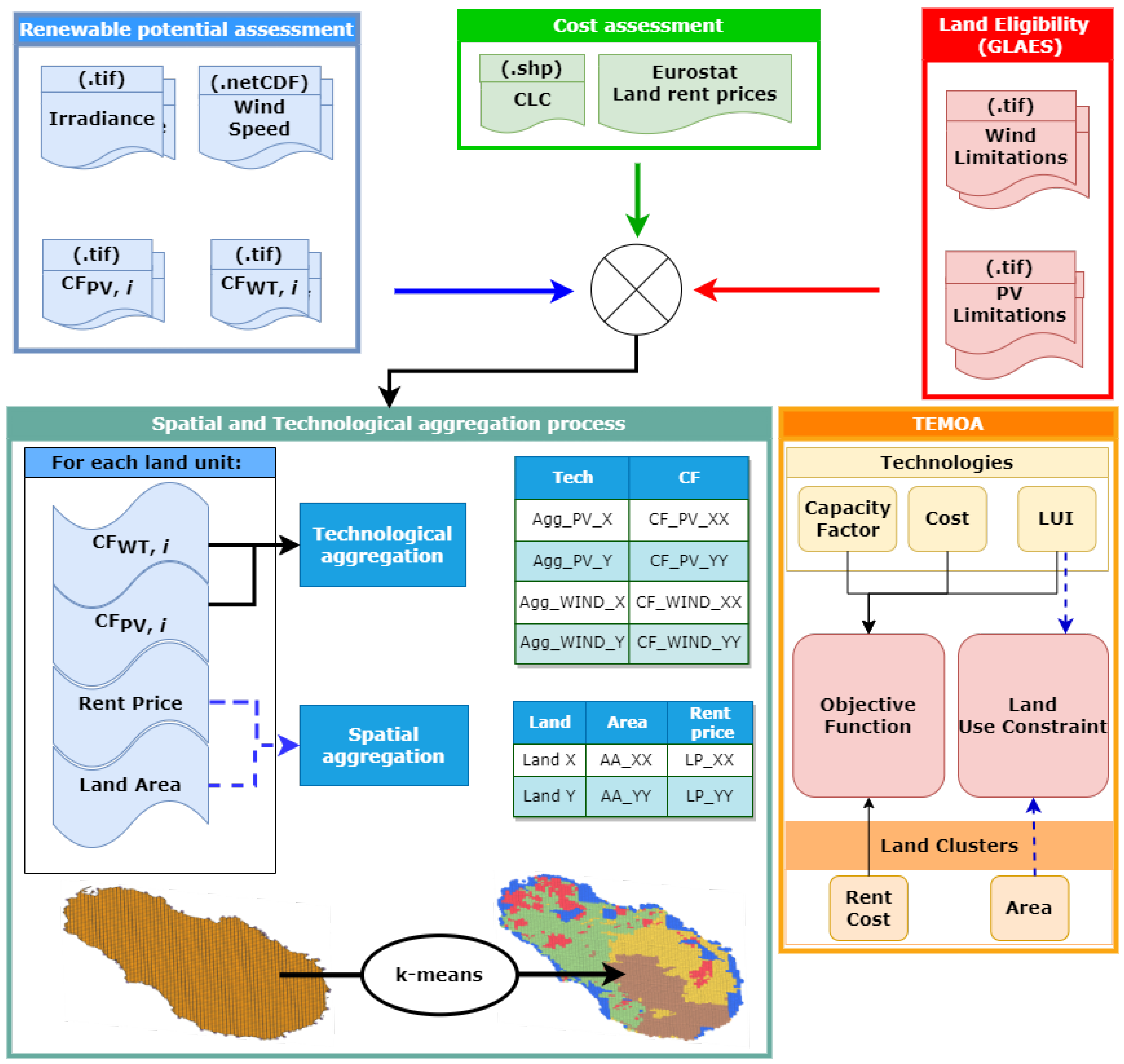
3.1. Modelling Framework

In this paper, the TEMOA [50] ESOM was selected, motivated by several key points:
  • Open source: TEMOA is open source, providing the transparency and customization needed for research. TEMOA’s code is written in Python and optimized in Pyomo, a Python library for optimization, so it has no accessibility constraints.
  • Similarity to other models: The TEMOA model formulation is like the model generators MARKAL/TIMES [11,51], MESSAGE [52,53], and OSeMOSYS [54]. Such tools, already commonly used in energy planning (e.g., MESSAGE in Syria [53], OSeMOSYS in Colombia [55], TEMOA-US [16]. Moreover, TEMOA is a validated tool whose convergence with the well-established TIMES framework has already been demonstrated in an Italian modelling instance [56].
The central component of the TEMOA framework is a technology-explicit description of the energy system model [57]. The energy system is described algebraically as a network of linked processes that convert energy feedstocks (e.g., coal, oil, biomass, uranium, sunlight) into end-use demands (e.g., lighting, transportation, water heating) through a series of one or more intermediate energy forms (e.g., electricity, gasoline, ethanol). The system consists of three demand-side sectors (buildings, transportation, and industry) and supply-side sectors (the upstream and the energy sectors) [57]. While the demand sectors consume energy to meet the final demand for energy services, the supply sectors produce the energy products consumed by the demand side (i.e., fossil fuels, primary renewable potential, electricity, and heat) [57].
TEMOA tackles an optimization problem comparable to standard TIMES models [58]. This problem involves minimizing the objective function, which represents the total cost of the energy system (denoted as C t o t ). The total cost, calculated in Equation (1), depends on the discount factor ( D i s c o u n t F a c t o r , representing the discounted value to the beginning of the time horizon of a unitary payment) and the cost values of individual technologies chosen in the optimal technology mix. Three key parameters in technology modeling play a crucial role in computing the objective function: investment cost ( C o s t I n v e s t r , t , v [M€/cap.]), fixed operation and maintenance (O&M) cost ( C o s t F i x e d r , p , t , v [M€/cap.]), and variable O&M cost ( C o s t V a r i a b l e r , p , t , v [M€/cap.]). While investment cost and fixed O&M cost are linked to a technology’s installed capacity, the variable O&M cost is tied to the total flow of output commodities. The L A r , t , v is factor used to annualize a technology’s investment cost, determined by the process-specific loan length and discount rate.
C t o t = C l o a n s + C f i x e d + C v a r i a b l e = r , t , v C o s t I n v e s t r , t , v L A r , t , v D i s c o u n t F a c t o r   C a p r , t , v + r , p , t , v C o s t F i x e d r , p , t , v D i s c o u n t F a c t o r   C a p r , t , v + r , p , t , v C o s t V a r i a b l e r , p , t , v D i s c o u n t F a c t o r   s , d , i , o F O r , p , s , d , i , t , v , o

3.2. Case Study: The Pantelleria Island

Selecting a case study in energy modelling is a crucial step in conducting an accurate and meaningful analysis. In this regard, the following criteria were considered for the selection of the case study:
  • Consistency with research objectives: As stated in Section 1, the focus of the analysis is to test the effectiveness of a spatially explicit model on a small scale. This defines the size of the area to be studied. In addition, it was specified that the suitability phase of the land can be an important factor in reducing soil availability. Therefore, the selection of a critical context from this point of view is necessary.
  • Territorial and technological diversity: According to Stolten et al. [28], the benefit of spatially explicit planning is higher if the territory under analysis presents geographical differences from the point of view of the distribution of energy resources and possible land uses. For this reason, the choice of a small area with characteristics of diversity is a fundamental element.
  • Data availability: The analysis is more significant if the data (both for the phase of the suitability of the land and for the estimation of the energy potential) are present and at high resolution.
  • Availability of modelling instances: The presence of existing and validated models on the chosen platform represents a strong added value in terms of the reproducibility of the study.
Considering the selection criteria listed above, the Island of Pantelleria was selected as a case study, thanks to its properties of territorial diversity [59]; the numerous data sources at the regional [60], Italian [61], and European levels; [CLC]; the existence of other studies with the same focus [62,63]; and the presence of an established model instance (TEMOA-Pantelleria) [64]. Below, the main features of the island of Pantelleria and the TEMOA-Pantelleria model used for the analysis are described.
In Figure 2, the island of Pantelleria’s energy density for both wind and PV is shown. The island is centrally positioned within the Strait of Sicily. Specifically, Pantelleria is situated at 36.785° latitude and 11.992° longitude, a geographical coordinate that underscores its pivotal location within the Strait of Sicily. This geographical circumstance yields meteorological conditions rendering Pantelleria an exceptionally auspicious site for the harnessing of variable renewable energy sources (VRESs). Pantelleria presents a consistently elevated level of solar radiation throughout the year, amounting to approximately 1500 kWh/m2. This abundance of solar irradiance is instrumental in the island’s clean energy transition agenda, affording substantial potential for solar energy generation. Additionally, the island experiences a substantial and dependable prevalence of wind, predominantly originating from the northwest, with wind speeds averaging around 7 m per second at an elevation of 25 m above sea level. All these climatic factors, in conjunction with the strategic location, position Pantelleria at the forefront of sustainable energy exploration and underscore its critical role in advancing clean energy initiatives [59], making it a compelling case study in the pursuit of land and energy sustainability.
The Pantelleria energy system is subdivided into five sectors (three demand-side sectors and two supply-side sectors) [65]. The demand-side sectors are buildings (including the agriculture, commercial, and residential sectors), transport, and commercial. The supply-side sectors are the power sector and the upstream sector. Each sector includes a set of technologies, characterized by several techno-economic parameters, used to produce all the commodities necessary to ensure the production of the required final energy service demands. The upstream sector includes fossil fuel import and internal production of biomass, as well as a fictitious commodity representing renewable energy. The output commodities of the upstream sector (along with fuel imports) are inputs for the power sector and the demand-side sectors.
To perform future projections in the different sectors, the model relies on a database of existing and innovative technologies (both at commercial and research and development stages), while future service demands in each sector of the economy (e.g., driven distance by car or truck, residential/commercial space heating, industrial production of steel or paper, etc.) are projected according to a set of drivers and demand elasticities and must be satisfied by the model at each time step. Future projections are articulated over several time steps, some of which are used for the model calibration and some others (set at the years 2025, 2030, 2040, and 2050) for the scenario analysis.
While the annual value of each final service demand of the model is known at the base year and projected along the time with exogenous drivers and elasticities, the intra-annual distribution of the demand is also important to consider seasonal and daily variations in environmental conditions that affect the energy demands. The division of the milestone year into more refined time slices is performed in TEMOA-Pantelleria with 4 seasons (spring, summer, fall and winter) and 3 times of day (day, night, and peak), leading to 12 time slices per year.

3.3. Geospatial Data and Tools for Land Eligibility and Energy Potential Analysis

In this paper, two macro-categories of data are used, namely, simple spatial data and spatiotemporal time series. Spatial data are represented as a list of numbers using a particular coordinate system. For example, the objects of an electronic map are represented using spatial data (roads, buildings, windspeed by location), represented as points and shapes with a specified position. In this analysis, spatial data are both the constraints used to perform the land eligibility analysis and, in general, all the spatial properties that are fixed during time (e.g., cost of land rent). The superimposition of the different thematic layers (e.g., administrative, or physical constraints) allows for the draw of the final land eligibility map. These kinds of data are fixed among all the scenario periods; therefore, they are applied once and do not change over time. On the contrary, spatiotemporal time series, related to the resource potential for both photovoltaic and wind, is time dependent. A georeferenced time series keeps the whole history of the evolving object over a period [66]. Typical examples include the monitoring of crop health over years [67] and meteorological time-series [68].
For the manipulation of both types of data, the use of geographic information system(s) (GIS) is mandatory. A GIS is a specialized tool designed for the organization and management of diverse datasets associated with geographic or spatial coordinates, utilizing a specific map projection system [23]. In our research, we employ the QGIS 3.10 software package [24] for handling, analyzing, and visualizing spatial information. GIS technology plays a pivotal role in spatial energy planning, as it enables the amalgamation of data about renewable energy resources, regulatory guidelines, and natural constraints.

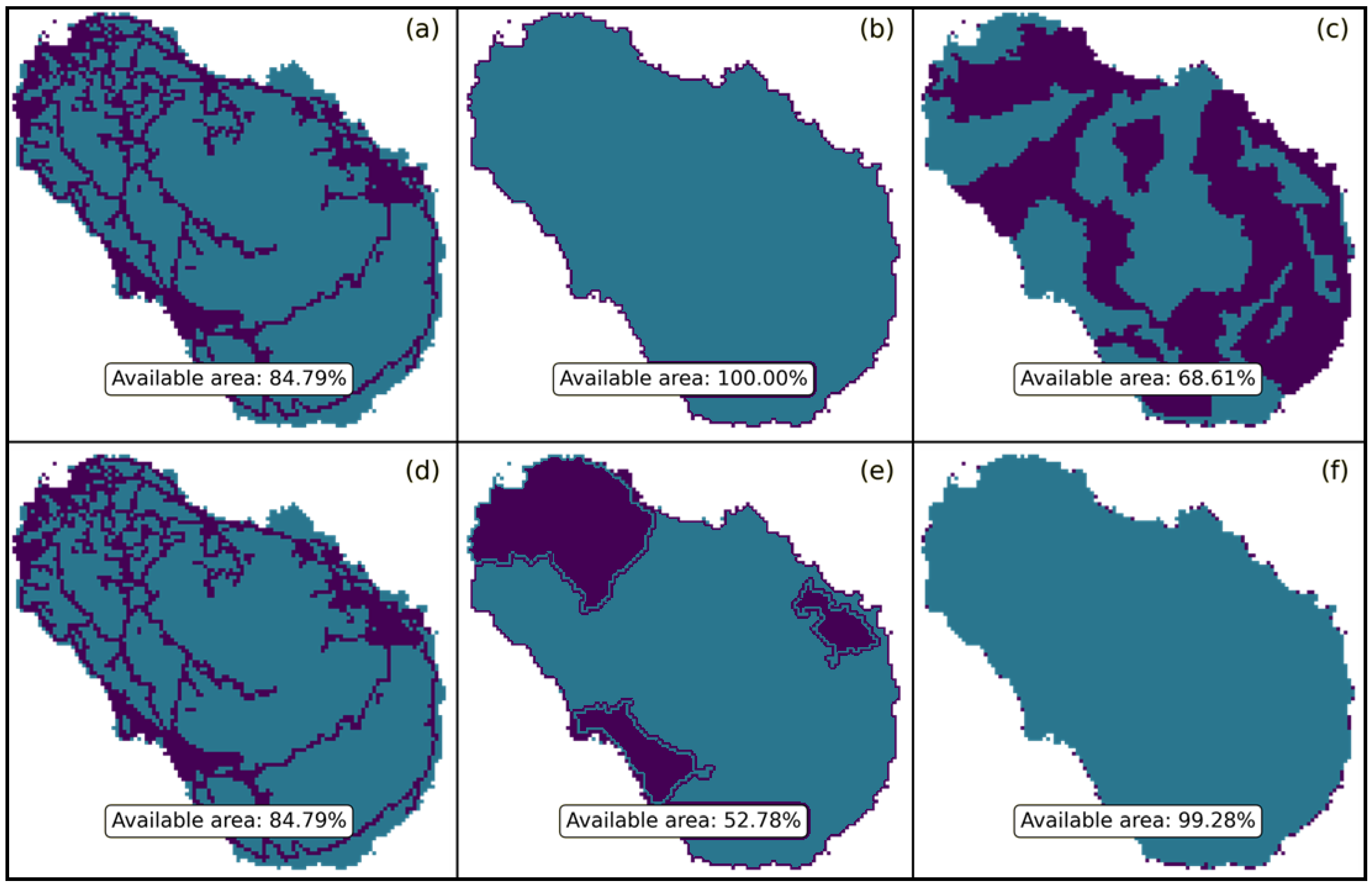
3.4. Land Eligibility Analysis

The existing literature extensively discusses eligibility criteria, and although specific aspects may vary, there is a consensus on its broad scope. Thanks to a review of the main analysis of this topic (as summarized in Table 1), it becomes evident that several consistent exclusion components are commonly considered. These include economic factors, administrative and technical considerations, and social aspects. Thus, it is expected that a study aligned with the existing body of knowledge should incorporate these elements as essential components when assessing the eligibility of land for renewable installations.
It is evident from Table 1 that all the pertinent research concurs on the existence of two primary clusters, about administrative and technical constraints. Administrative limitations typically encompass regions where the establishment of new facilities is prohibited for various reasons, including natural protected areas [73], proximity to historical sites [74], and residential agglomerations [75]. On the other hand, technical constraints are predominantly linked to challenges in constructing or operating new facilities due to factors such as terrain and soil conditions [76] or adverse weather patterns (e.g., low wind speeds, shadowing effects from hills and mountains). Additionally, these factors may also exert an influence on economic constraints, as there are overlaps between technical and economic characteristics, including criteria such as wind speed thresholds and slope thresholds. As underscored by McKenna et al. [71], there is a pressing need within the literature for the validation of studies related to land eligibility. Furthermore, there appears to be a notable absence of social and political considerations in the existing analyses. Consequently, the adopted criteria and their associated clusters are reported in Table 2.
According to the constraints in Table 2, land availability is constrained by environmental/technical criteria, thereby rendering the construction phase of the plant unfeasible due to adverse soil conditions and distance from the grid. Similarly, operational convenience for the plant is compromised due to low resource availability. Data about resource availability are distinctly derived for wind and photovoltaic sources and are more comprehensively discussed in the resource assessment phase. Information concerning crop types and soil conditions is obtained from the Corine Land Cover source [76], a widely recognized reference in the literature, corroborated by GLAES [21]. Data not accessible through extensive, open-access databases are sourced from localized Italian studies. The sole exception pertains to the grid distance, which is unavailable in both large databases and local studies.
Administrative and habitat constraints, predominantly driven by natural preservation objectives, are derived from Natura 2000 [80] and the World Database of Protected Areas (WDPA) [74]. Natura 2000 serves as the principal instrument of European Union policy for biodiversity conservation, while WDPA stands as the most exhaustive global database encompassing marine and terrestrial protected areas.
Lastly, for anthropic limitations, data are extracted from OpenStreetMap (OSM) [75], an open-access global database characterized by public participation during data collection. In Figure 3 the different limitation categories, for both wind and photovoltaic technologies, are reported. For the solar resource, its land availability is mainly eroded by anthropic and environmental limitations (~15% and ~31% of unavailable land, respectively), while there is no specific constraint due to natural habitat and historical heritage. Considering the overlapping of categories, the final available area results in ~35%. Differently, for wind, the main limitations are habitat (~51% of land made unavailable due to Natura 2000 [80]) and again, the anthropic one. This results in an overall ~10% of available land.

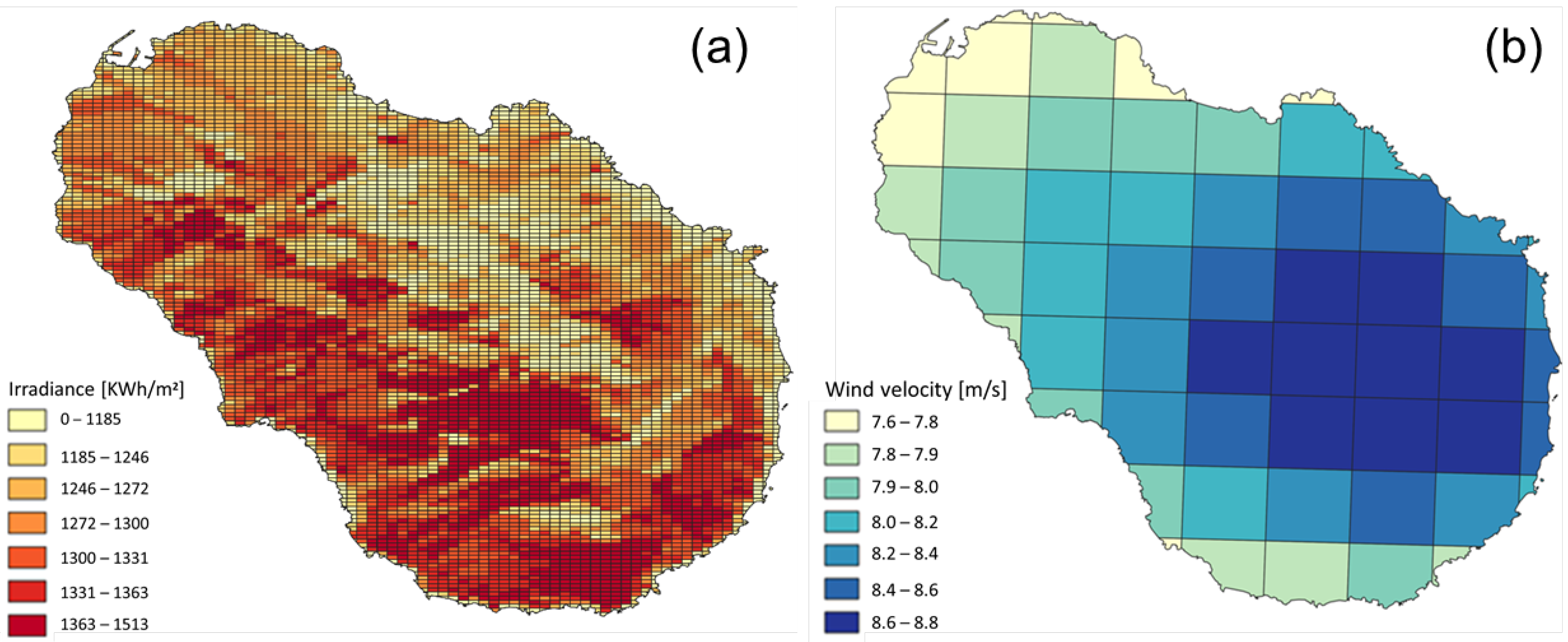
3.5. Potential Assessment

The way solar and wind resources are assessed should be in line with the most recent and well-established existing literature. As highlighted by McKenna et al. [71] in the abovementioned review, the technical potential assessment requires a standardization of the analysis and the tools. This is justified by the need for reproducibility and data availability. To accomplish these requirements, solar and wind technical potentials are estimated using the calculation methodology of Elkameen et al. [81]. Technical potential is estimated starting from solar irradiance and wind speed data and, after some passages, obtaining the capacity factor for the different sites. The detailed steps are described in the specific photovoltaic and wind assessment sections, respectively.
The starting point for this paper is the choice of the data sources for the potential assessment. This practice must be in line with the needs of the analysis (e.g., extension of the area under study, temporal horizon, model resolution) [28]. Therefore, after having fixed the methodological steps, a detailed analysis of all the possible data sources for both wind and photovoltaic was conducted.
Solar radiation and wind speed can be estimated in two different ways [71], through a database already providing the energy potential at a certain resolution, or through a detailed model considering slope, aspects, shadowing effects, and roughness of the terrain to calculate the potential. Concerning the former, the analysis is conducted both considering large global databases and national-specific ones.
The results are summarized in Table 3, presenting a classification of the main database for solar and wind technical potential assessment. Sources are characterized according to data typology, cover, and resolution. For these last two items, data are also differentiated by temporal and spatial attributes. Sources belong to the following classes:
  • Observation: The observational approach entails the acquisition of empirical data from weather stations and measurement devices, providing invaluable insights into contemporary weather patterns, wind speed observations [82], and solar radiation measurements [83].
  • Reanalysis: The reanalysis methodology integrates numerical weather prediction models with observed datasets, yielding comprehensive datasets encompassing various meteorological parameters [71]. Examples include ERA5 [84] and MERRA2 [85], which serve as reputable sources for historical climate data assessment in wind resource studies, while similar data sources exist for solar energy assessments [86].
  • Climate models: Climate models from initiatives like the Climate Model Intercomparison Project (CMIP) and CORDEX simulate future climate conditions, facilitating the assessment of wind and solar resource variability in response to long-term climate changes [87,88]. These models are instrumental in understanding the potential impacts of climate change on renewable energy resources.
  • Atlas: Wind and solar atlases, exemplified by the New European Wind Atlas (NEWA) and the Global Wind Atlas (GWA), offer high-resolution spatial information regarding energy potentials in specified regions [89,90]. These atlases play a crucial role in renewable energy planning and development by providing detailed assessments of wind and solar resources.
Table 3. Data sources for general and technology-specific resource assessment. Characterization by spatial and temporal coverage and resolution.
TechnologyData TypologyDatabase NamesCoverageResolution
SpatialTemporalSpatialTemporal
GeneralObservationHadISD [83], Tall Tower Database [82]GlobalHistorical, 20–50 yearsSite-specific5 min–1 h
ReanalysisMERRA-2 [85], ERA5 [84]GlobalHistorical, 40–70 years30–60 km1–6 h
Climate modelsCMIP5 [87],
EUROCORDEX [88]
GlobalHistorical and future, 80–250 years10–300 kmHourly–monthly
SolarAtlasGSA [91], SolarGIS [92]GlobalHistorical90 m0.5–1 h
ReanalysisHelioClim-3 [86]GlobalHistorical and real-time3 km15 min–1 h
WindReanalysisNEWA [89], DOWA [93], RSE [61]Regional (EU)Historical, 11–30 years1.5–3 km0.5–1 h
AtlasGWA [90]GlobalHistorical average50–200 mN/A
ReanalysisWINDographer [94], Mesonet [95]USAHistorical3 kmHourly
Most of the databases are made available at a global level, even if one exception is found for the New European Wind Atlas (NEWA), which has a European focus. In terms of temporal coverage, atlases are the most limited since they only provide historical average or single-year data. For both observation and reanalysis, the timeframe is wider (from 10 to 70 past years). Finally, climate models are the only ones capable of providing future projections, even if there are non-negligible errors in model forecasts [71]. The limitation inherent to databases, whether they are global or local in scope, is their inherent inability to accommodate site-specific factors that exert a discernible influence on energy potential. In regions characterized by intricate topographical features, such as fluctuations in elevation, surface orientation (including slope and aspect), and the presence of shadows, pronounced local gradients in energy distribution become manifest [96,97]. Consequently, it becomes imperative to employ models capable of incorporating local considerations into energy estimations. In this context, the availability of hourly time series at a microscale resolution (~1.5 km) made available by RSE represents a pivotal step, and this has motivated the selection of it as a source for wind potential of this analysis. It is worth noting, however, that the sources of solar data under examination do not inherently furnish specific microscale considerations. Consequently, the utilization of comprehensive models becomes indispensable for accounting for these intricacies. The existing literature offers a variety of potential approaches. Notably, the “r.sun” algorithm, a development within the GRASS-GIS framework [98], stands out as a robust contender, as it calculates solar radiation at an hourly resolution when supplied with a digital elevation model (DEM) corresponding to the target region. Additionally, ArcGIS [99] provides a solar radiation toolbox [100], which operates similarly to r.sun and has undergone calibration and validation through international research endeavors [101]. The advantage of r.sun is the number of users it has already reached, and so, the number of calibrations and validations this tool has undergone [102]. Therefore, for solar potential assessment, r.sun was selected, applying the methodology described in the work of Gasparovic et al. [103].

3.5.1. Photovoltaic Potential Assessment

To assess the yearly potential conversion capacity of a photovoltaic (PV) power facility, denoted as A E P P V , within a specific grid cell, denoted as “i” we employed Equation (1) [81]. This calculation hinges on both the available solar resources and the specifications of the solar modules in use. Additionally, we determined the capacity factor, C F P V , for PV systems within the grid cell “i” using Equation (2) [81]. This factor signifies the actual electrical output that a PV power plant could generate at its designated location over a given time frame when compared to its theoretical maximum potential output, assuming uninterrupted operation. This capacity factor calculation considers technology-specific parameters and the accessibility of location-specific resources, thus enabling performance comparisons across different sites before the installation of PV systems.
A E P P V , i = G H I i × η P V × P R × A P V , i
C F P V , i = A E P P V , i P P V , r a t e d × T
In Equations (2) and (3),
  • GHIi represents the average global horizontal irradiation (kWh/m2/time).
  • APV,i indicates the area within grid cell “i” suitable for PV implementation (km2).
  • ηPV represents the efficiency of the PV module in converting sunlight to electricity, with an assumed value of 21% [81].
  • PR denotes the performance ratio for the solar module, set at 0.85 [81]. This ratio accounts for the disparity between performance under standard test conditions and the actual system output, factoring in losses due to conduction and thermal effects.
  • T signifies the total number of hours in a year, equivalent to 8760.
  • PPV,rated represents the power density or of the solar PV system. For this study, we employed a value of 32 MW/km2 for a fixed-tilt utility-scale solar system using mono-crystalline silicon cells, which is the most common in the actual market [104].
The G H I is derived from r.sun starting from a digital elevation model (DEM) with a 10 m resolution. Subsequently, the original irradiance has been corrected for atmospheric attenuation based on the clear sky coefficient ( k c s ) as in Equation (4) [81].
G H I = G H I × k c s
TEMOA time slices are categorized into seasons, each comprising days, nights, and peak periods. As there is no sunlight during the night, the capacity factor (CF) is uniformly assumed to be zero for all seasons. Consequently, our focus narrows down to determining the seasonal CF values for two distinct periods: day and peak. This entails computing eight capacity values. For each of these, we applied Equations (2) and (3), substituting the term “GHI” with the solar radiation received during the validity period of the capacity factor and the term “T” with the hours specific to that period. Aggregated solar radiation for the specific “T” period is obtained starting from the hourly irradiance (W/m2) and integrating all along the period T. Moreover, r.sun requires specifying a reference year on which the calculation is performed. Since the aim is to compare different lands under the same atmospheric conditions, the yearly variability of solar irradiance is neglected, and 2020 values are assumed constant.
Another remarkable hypothesis is related to the division between day and peak production. As specified above, within a season, a day might have various times of interest. For instance, the peak electrical load might occur at midday in the summer, and a secondary peak might happen in the evening. This division should be accounted for when evaluating the photovoltaic potential since the mismatch between producibility potential and demand is one of the main problems with VRESs [105]. Seasonal daily and peak capacity factors under the assumption described are reported in Figure 4.
The presented box plots reveal that spring and summer exhibit higher median capacity factors compared to autumn and winter, indicative of a stronger solar potential during these warmer seasons (36% and 52% concerning 31% and 17%). These periods also display broader capacity factor ranges, likely influenced by intermittent cloud cover or variations in solar incidence angles. Notably, summer stands out with occasional exceptionally high-capacity factors, attributed to optimal sun angles and longer daylight hours. In contrast, the winter season demonstrates a compact interquartile range (IQR) and lower median, reflective of shorter days and lower sun angles. Lower-end outliers in winter may indicate days with minimal solar irradiance due to adverse weather conditions. The “Peak” period capacity factors also follow a seasonal trend, with spring and summer consistently outperforming autumn and winter. However, “Peak” distributions are narrower across all seasons compared to “Day” distributions, highlighting the reduced susceptibility of peak sunlight hours to diurnal and weather-induced fluctuations. Overall, these insights emphasize the critical importance of understanding the temporal variability in PV capacity factors for optimizing solar energy system planning and performance.

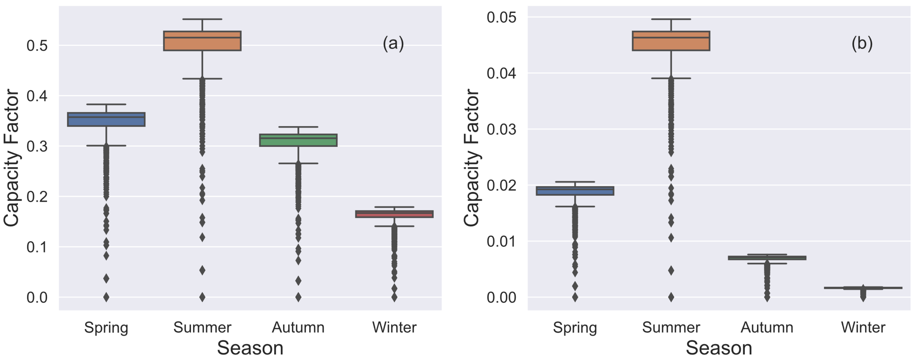
3.5.2. Wind Potential Assessment

The RSE AEOLIAN platform provides wind speed data at heights of 50, 75, 100, 125, and 150 m above sea level (a.s.l.) [61]. These values correspond to the most representative hub heights for both currently installed onshore wind turbines and future potential installations both on land and at sea. As was carried out for solar potential calculation, the goal is to obtain capacity factor values for each time slice of the model. This primarily involves translating hourly wind speed data into site-specific energy production.
The site-specific energy production calculation is achieved by combining the historical time series (or probability density function) of wind speeds at the hub height of the wind turbine with the power curve of the specific wind turbine of interest, also expressed as a function of wind speed at the hub’s height. Theoretically, to calculate site-specific energy production, one should use many power curves and compute a representative average. However, due to difficulties in obtaining a representative set for data availability issues, the site-specific energy production analysis was conducted using a single wind turbine model for each hub height. We considered the three lower hub heights: 50, 75, and 100 m a.s.l., along with three commercially available wind turbine models accessible online. Table 4 provides the main characteristics of the three wind turbines used for the calculation at the considered hub heights:
Table 4 presents key specifications of WTG models at varying hub heights, ranging from 50 to 125 m. Notably, it reveals the increasing nominal power and rotor diameter as the hub height elevates, which is essential information for optimizing wind energy production at different altitudes. It also must be noticed that wind references and hub heights differ. Therefore, there is an error introduced by the wind speed at the data level with respect to the real height at which the wind turbine is installed. Nevertheless, considering the power law at which wind speed variation is subjected [107], it has been checked (not shown) that the producibility errors are always below 5%.
The turbine’s power generation E W T , i [MWh] in the time slice “i” was estimated by combining the Rayleigh wind speed distribution, the WT’s power curve collected from the manufacturer, and the number of hours in operation during a time slice in line with TEMOA-Pantelleria time slices, as in Equation (5).
E t , i = μ T L W T V = V c u t i n   V = V c u t o u t P V d V  
where P V  is the power curve of the selected wind turbine as a function of wind speed at a given hub height, T is the number of hours in a time slice, P n o m i m a l , t is the rated power of the selected turbine (MW), V c u t i n is the cut-in wind speed of the turbine (4 m/s), V c u t o u t  is the cut-in wind speed of the turbine (25 m/s), and L W T is the percent of the electricity losses in wind generation system (0.85). In addition, μ is the turbine availability factor (0.97). After knowing the time slice production, the capacity factor for time slice “i” for turbine “t” was calculated as in Equation (6):
C F t , i = E W T , i P n o m i m a l , t × T
The results of this process are shown in Figure 5.
In Figure 5, two different kinds of patterns are observable. The analysis reveals distinct seasonal and daily patterns in wind turbine capacity factors. Across all turbine heights, winter consistently displays approximately 20–25% higher capacity factors compared to summer, notably pronounced during nighttime slices. In comparison to summer, autumn showcases marginally elevated capacity factors, approximately 10–15% higher, especially evident during day and night periods. The impact of turbine height is observable with a consistent increase in capacity factors across all seasons, with higher heights indicating approximately 15–20% better performance. Moreover, the variability within each season and time slice remains relatively consistent, with night periods displaying notably wider ranges than a day. Outliers, though sporadic, suggest instances of extreme deviations in capacity factors.

3.5.3. Cost Assessment

The potential assessment phase determines the operational yield of the plant. Nevertheless, when seeking to differentiate various land types for capacity expansion plans, technical potential is not the only influencing parameter. According to the International Renewable Energy Agency (IRENA) 2021 report [108], the levelized costs of electricity (LCOE) of the renewable installations is mainly determined by capacity factors, investment costs, operations and maintenance (O&M), and auxiliary costs. Since the purpose of spatially explicit energy planning is to consider geographic aspects capable of influencing ESOM outcomes [29], it is necessary to identify which of the abovementioned voices are spatial-dependent.
For capacity factors, this aspect has already been addressed. Coming to costs, when faced with the decision between lands of equal potential, the cost of the land (by rent or acquisition) and the expenses associated with its connection to grid infrastructure become pivotal factors [108].
To consider the trade-off with other sectors, the cost of land is assumed to be equal to the agricultural land price. Agricultural land rents refer to the price of renting one hectare of agricultural land without buildings or plantations for one year. These data are derived from a Eurostat analysis [109] dated 2021 with a spatial scope of the whole European territory and a spatial resolution of country regions. Land price has been neglected for nonagricultural/dismissed land. The cost attribution follows the rule in Equation (7).
i f   C L C c l a s s =   A g r i c u l t u r a l   l a n d   ,     0.0216 < L P < 0.1714     M km 2       E l s e ,     L P = 0
where C L C c l a s s is the Corine land cover class of each particle and L P refers to land price. A significant variation of the L P is observed between the maximum and the minimum value, the former being around 10 times the latter. This is justified by the great diversity in the Italian territory. While the focus of this analysis is limited to Pantelleria Island, situated in Sicily, the Italian maximum and minimum land price values have been chosen in both the above discussion and for future utilization (as outlined in Section 3). Indeed, we have opted to utilize this range of land price values to conduct a sensitivity analysis within the model, with the final aim of testing the extent to which these components influence the outcomes of the model. Additionally, when transitioning land use from agriculture to energy, trade-offs in soil carbon balance must be considered. Properly accounting for these features can significantly impact overall cost assessments [110]. However, due to current limitations in ESOMs, the inclusion of these aspects is deferred until mature models capable of addressing land properties are available.
Finally, for the cost of connection, some concerns come with its accounting. First, according to the Italian Energy Transmission Authority (TERNA) [111], the specific point of connection (that determines the distance) is not known a priori, and strongly depends on design-specific considerations. According to plant size and desired output voltage, the connection can be performed at grid level or the primary cabin [111]. This introduces the first uncertainty in this cost estimation. Then, ESOMs generally do provide aggregated capacity for all the plants belonging to the same category [112]; therefore, it is not known how the aggregated capacity is discretized, with uncertainties also in the size term. Lastly, the detailed IRENA cost analysis of wind power technology [113] does not specify the distance from the grid as a pivotal factor in determining the connection cost.
Given the design-specific nature of grid connection costs and the challenges in estimating them accurately, we have chosen not to include them as a factor in our analysis.

3.6. Data Aggregation

At this stage of the analysis, the data about wind potential, solar potential, and costs, presented as geodata (shapefiles), that need manipulation to become compatible with the data structure of ESOMs [50] are the following: The solar domain, ( D s o l a r ) , is represented as a set ( S ) where each cell ( s S ) is characterized by different PV capacity factor time slices ( C F P V s , t s ) . Formally, this domain is expressed as in Equation (8):
D s o l a r = { C F P V s , t s | s S }
The same is valid for the data related to wind CF time slices as in Equation (9):
D w i n d = { C F   W I N D w , t s |   w W }
and land prices as in Equation (10):
D l a n d = { L P l | l L }
Notably, one significant challenge in data preparation arises from the divergence in spatial resolutions among the various datasets. A critical issue that emerges when attempting to overlay the different domains involved in the analysis is the lack of correct intersection of internal boundaries between them. This issue, also named the partition problem [114], is created by mismatched spatial resolutions and boundaries of the domains. Our approach lies in the synthesis of these domains into an intersection domain, ( D i n t e r s e c t i o n ) as from Equation (11).This domain is an amalgamation of the overlapping elements from ( D s o l a r ) ,     ( D w i n d ) ,     ( D l a n d ) , and is denoted as a set   ( I ) . Each element ( i I )   i n   ( D i n t e r s e c t i o n ) encapsulates the attributes from the intersecting cells of the individual domains:
D i n t e r s e c t i o n = { C F P V i , C F W I N D i , L P i | i I }
The aggregation of data into ( D i n t e r s e c t i o n ) , as explicated in Equation (12), is a pivotal step. For each cell ( i I ) , the attributes ( C F P V i ) ,     ( C F W I N D i ) ,     ( L P i ) are computed by an aggregation function that operates on the data from the overlapping cells in ( S ) ,   ( W ) ,   a n d   ( L ) :
C F P V i = Function C F P V s s   overlaps   with   i C F W I N D i = Function C F W I N D w w   overlaps   with   i L P i = Function L P l l   overlaps   with   i
At this point of the analysis, data are still a unique domain with different particles, each of them characterized by many geospatial attributes. Notably, the TEMOA model requires a data format that is not geospatially explicit. As with any other traditional energy system optimization model, TEMOA presents an aggregated description of the system, where the spatial features of technology (e.g., CFs and costs associated with the land particle on which they are installed) are not present. Indeed, CFs are defined in the model as in Equation (15):
C F r , p , t , v     w i t h     r R , p P , t T     a n d     v V
where r R refers to model regions, p P to periods, t T  to technologies, and v V to vintage. The same indexes are valid for costs. Therefore, it is necessary to have spatial attributes (location-dependent cost and capacity factor) referred to an index “land”. Integrating individualized PV and wind technologies for each land parcel, differentiated by unique cost and capacity factors, would theoretically work. Yet, this precision comes at the cost of an enormous dataset, rendering the model computationally intractable due to the vast number of parameters involved. To address this, an aggregation/clustering algorithm is employed to partition the domain into clusters with homogenized attributes. Within this framework, an established methodology, as presented by Stolten et al. [28], offers a structured workflow for transitioning from multiple variable renewable energy source (VRES) data to a limited number of aggregated technologies, each associated with a respective land cluster, representing the total available land area suitable for the installation of the corresponding technology. This framework, adapted to our work, is shown in Figure 1.
In the technological aggregation phase, photovoltaic and wind technologies are categorized based on their capacity factors (CFs) and cost characteristics. This categorization results in aggregated technology clusters, such as Agg_PV_X and Agg_WIND_Y, each with its distinct capacity factor and associated cost. Spatial aggregation, on the other hand, condenses geographical information into discrete land clusters. Each cluster, represented by a land type such as Land X or Land Y, is defined by its area and the cost of land use. These spatial clusters form the basis for the physical constraints within the model, dictating the potential for technology deployment across different geographical areas. Finally, in the model adaptation phase, the original TEMOA code is modified to account for land availability and for linking specific technologies at their belonging cluster.
The clustering of the geospatial cells among the selected attributes is performed with multiple algorithms to determine which one performs better. The three tested algorithms are HDBSCAN [115], Kmeans [116], and DBSCAN [117]. HDBSCAN, a hierarchical density-based algorithm, is adept at identifying clusters of varied density without the need for pre-specifying the number of clusters. Its approach is particularly suitable for geospatial data, which often exhibit heterogeneous density distributions due to the irregular spatial distribution of renewable energy resources. In contrast, Kmeans—simple and efficient—is a centroid-based algorithm, meaning that objects in the data are clustered by being assigned to the nearest centroid. However, a major pitfall of Kmeans is its lack of detecting outliers, or noisy data points, which leads to them being classified incorrectly. DBSCAN stands as a middle ground between the rigidity of Kmeans and the flexibility of HDBSCAN. By designating core points within high-density regions and expanding clusters from these cores, DBSCAN excels in discovering clusters with arbitrary shapes, an attribute of high value when dealing with spatially complex landscapes.
For the clustering algorithms requiring the computation of the distance matrix, a spatial sampling procedure is performed [118], clustering only the smallest subset of data. Then, the nearest neighbor [119] method is used to predict the cluster affiliation for the non-sampled particles. The performance of these algorithms is tested both by their clustering acumen and by their computational demands, as reported in Table 5. The silhouette score [120]—ranging from −1 to 1—has been used as a quantitative measure of cluster cohesion and separation. A high silhouette score indicates a clustering configuration where inter-cluster distances are maximized and intra-cluster distances are minimized, reflecting distinct and well-separated clusters that are integral for spatial analysis. Complementarily, computational time and memory usage are critical metrics for assessing the scalability of these methods. They provide insight into the algorithms’ operational efficiency and practicality for large-scale applications, where rapid processing and memory management are essential. The results of the clustering procedure for the three different algorithms are reported in Figure 6.
As appreciable in Table 5, Kmeans and DBSCAN outperform HDBSCAN in terms of silhouette score and memory usage, with Kmeans standing out as the best one in all the three metrics under analysis. The outstanding performance of Kmeans can be justified by the absence of outliers. Indeed, for both cost and renewable energy potential, the minimum value is zero where no installation is possible, and maximum values are constrained in a very similar range for all the data (there is no drastic resource variability along Pantelleria Island). Therefore, also considering the possibility of selecting clusters a priori, Kmeans is selected for this analysis. Moreover, the underlying hypothesis of Kmeans, that data must be globular and isotropic, is verified considering the high value of the silhouette score.
Considering Figure 6 is shows how HDBSCAN and DBSCAN are more flexible in terms of cluster shapes, which is evident from the varied shapes and sizes of clusters. Kmeans, on the other hand, assumes the clusters are spherical, leading to more uniform and rounded clusters. In terms of noise, HDBSCAN and DBSCAN can identify outliers inserting them in the (−1) cluster, even if very few elements are present in this category (checked, not shown). The final number of clusters is another pivotal parameter in this analysis. In Kmeans, it is imposed at 5, while the other methods reach 11 (HDBSCAN) and 17 (DBSCAN) clusters. In this case, especially for DBSCAN, the clusters are very fragmented and some of them appear to contain few elements.
In conclusion, since the aim is to identify macro-areas characterized by similar energy properties and to have a method as scalable as possible, Kmeans still guarantees the best outcome.
The refinement of geospatial data through clustering algorithms has yielded a comprehensive set of land and technological clusters, each distinctly characterized by both spatial and technological attributes. We define the clustered domain, ( D c l u s t e r e d ) , as the outcome of applying clustering algorithms to ( D i n t e r s e c t i o n ) . This domain comprises a set of clusters ( C ) , where each cluster ( c   C ) represents a group of cells with similar characteristics. The attributes of each cluster are derived from the aggregated attributes of its constituent cells. Specifically, the average photovoltaic capacity factor C F P V c , average wind capacity factor C F W I N D c , and average land price L P c  are calculated for each cluster, using Equations (14)–(16):
C F P V c = 1 c i c C F P V i
C F W I N D c = 1 c i c C F W I N D i
L P c = 1 c i c L P i
In these expressions, ( c ) denotes the number of cells in cluster ( c ) . Furthermore, the total land area of each cluster is determined by summing the areas of all cells within the cluster.

3.7. Model Integration

After the data aggregation procedure, a reduced set of land and technological items is made available for model integration. In this context, there are two optimization goals. The first is to install the renewable energy technologies on the “best” cluster, where “best” denotes the cluster identified by the ESOM following the least cost optimization.
The second objective is to have a renewable energy installation development compatible with the land limitations of Pantelleria Island. Therefore, the ESOM must be capable of using the inputs of the clustering phase (technological parameters for renewables, land price, and area for land clusters) to determine the optimal deployment of technologies across different land clusters. To achieve this goal, it is necessary to bring some modifications to the TEMOA code:
(1)
Insert in TEMOA a new set that describes the land resource. Traditional ESOM elements (mainly process and commodities) do not allow for proper land representation. Indeed, it would be wrong to model the land consumed by plant installation as a commodity or a technology, for two main reasons. First, a commodity is something that is exchanged between processes as input or output. Here, the role of land is to host its associated technology (at certain conditions of capacity factor and cost) for its lifetime. Second, commodity consumption is related to the activity of a plant, passing through its efficiency (e.g., natural gas consumption proportional to combined cycle plant activity). In this case, land is consumed when new capacity is installed and becomes available as soon as the installed technology on that land dies. As depicted in Equations (17) and (18), the new TEMOA set is called L a n d   C l u s t e r , for which a L a n d   A r e a c value is associated, describing the available area for the land cluster “c”.
S e t = L a n d   C l u s t e r   ( L C )
A t t r i b u t e = L a n d   C l u s t e r l
(2)
Insert in the model a new parameter and new constraint, linking the capacity installation to land consumption. Indeed, as shown in Equation (19), the land use intensity (LUI) parameter acts as a critical bridge linking the land clusters “ L C i ” with the applicable technologies “j”. It quantifies the amount of land required for the installation of a unit of technology (e.g., a megawatt of wind or solar power). The LUI parameter ensures that the model’s solutions are not just economically optimized but also spatially feasible. If an LUI is not defined for a specific technology within a given land cluster, it implies that the technology cannot be installed in that cluster, thereby introducing a direct spatial constraint into the optimization process.
L a n d A r e a c r , t L U I r , t , v c C a p r , t , v
According to the TEMOA optimization module, thanks to Equation (19), the model has several opportunities to consume land area to install photovoltaic or wind plants, but the convenience is determined by the capacity factor of the process. The objective function of Equation (1) already brings the model to select the technologies with the best capacity factor, because this is directly reflected in the cost. Nevertheless, the land consumption and its related cost is not accounted for. Therefore, the objective function is modified as follows (Equation (20)):
C t o t = C l o a n s + C f i x e d + C v a r i a b l e + C l a n d = r , t , v C o s t I n v e s t r , t , v L A r , t , v D i s c o u n t F a c t o r   C a p r , t , v   + r , p , t , v C o s t F i x e d r , p , t , v D i s c o u n t F a c t o r   C a p r , t , v + r , p , t , v ( C o s t V a r i a b l e r , p , t , v D i s c o u n t F a c t o r   s , d , i , o F O r , p , s , d , i , t , v , o ) + r , t , v L P r , c , v L U I r , t , v c C a p r , t , v
where the additional term r , t , v L P r , c , v L U I r , t , v c C a p r , t , v accounts for cost of land caused by the installation of C a p r , t , v by the technology t at vintage v, which causes consumption proportional to the L U I r , t , c on the cluster c. This consumption, finally multiplied by the land price L P r , c , v of the cluster, moves the total cost. In conclusion, the accounting of land price is solved through an objective function modification as in Equation (20). The rational use of land, considering limitation is reached by Equation (19), makes it now possible to extract information about the better clusters for renewable installation, given that the plant location is accounted for in the model.

4. Results

This section presents a comparative analysis of energy scenarios derived from two modelling approaches: one integrating the advanced land feature considerations previously described, and a conventional one. The objective is to test the hypotheses stated before about the advantages of spatially explicit energy planning.
Section 4.1 introduces the initial findings, highlighting the advanced technological and spatial characterization introduced by the previous analysis. Activation of the land use constraint and land price components, as discussed in Section 4.2, leads to different final ESOM scenario configurations.
The Discussion section (Section 5) elucidates the role of spatially explicit planning in optimizing the siting of energy facilities and efficient land use. These findings highlight the importance of spatial consideration in improving the efficacy of energy planning.

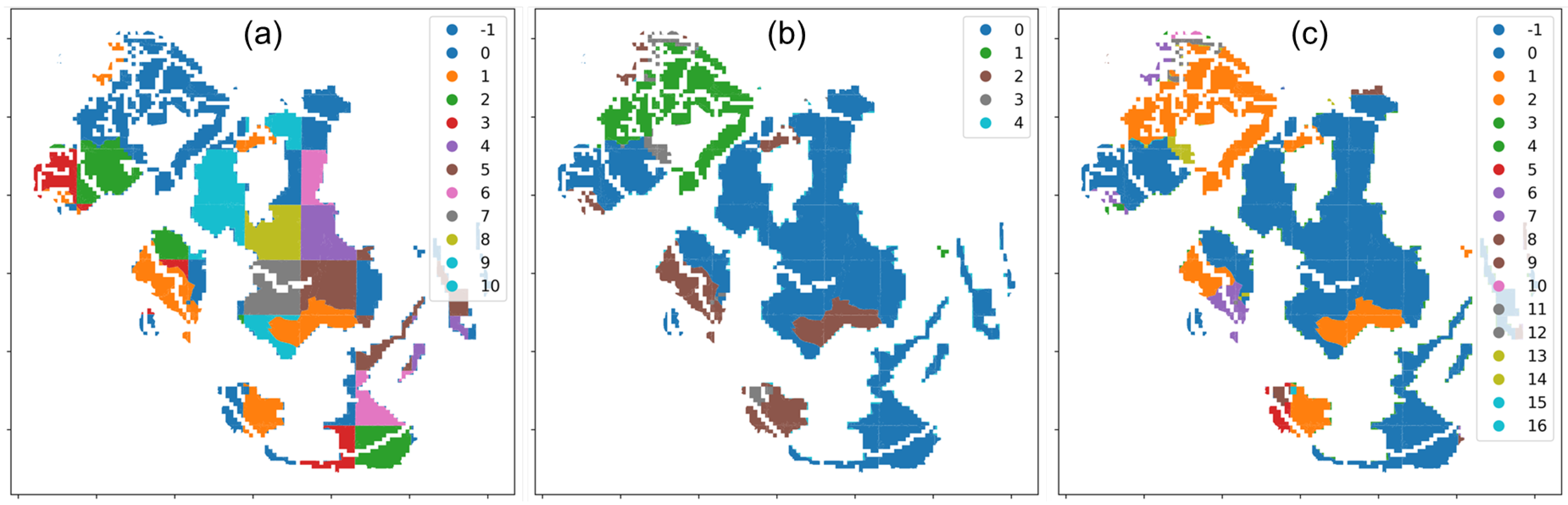
4.1. Technological Clustering Results

The two configurations of the model here analyzed are the traditional one (no land use module activation) and the new one (land use module activated). In both the model configurations, the wind and photovoltaic capacity factors result from the technological discretization previously explained (Figure 7, resulting from Section 3.5.1).
In Figure 7, those clustered capacity factors are reported and compared with the average ones to highlight the improvements brought by the cluster analysis carried out. In the land cluster description, the available area and the installable technologies on the cluster are highlighted (Table 6). As mentioned above, the limitations introduced by Table 6 for the installation of specific technologies on certain clusters and the land price accounting in the objective function are present only in the TEMOA-Pantelleria land-explicit configuration. Discretizing technologies based on their spatiotemporal attributes brings non-negligible advantages in terms of technological options for the model, which may cause a lower total cost of the system. Considering the relative difference between the old and the new technologies, is possible to observe values around 10% (summer and spring wind peak). Therefore, according to the sign of the difference, the model overestimate/underestimates the installed capacity of the same amount. Strongly influencing the cost. This consideration is further explained in the following graphs. Still related to the cost, it is possible to see the impact of the spatial aggregation on the land side, when the rent cost is added, as shown in Table 6.
Table 6 reports the resulting land clusters from the Kmeans algorithm (Figure 6b) and their associated technologies, whose technical attributes are reported in. The only difference between Figure 6b and Table 6 is that the fourth cluster has been deleted since it presents zero potential for both photovoltaic and wind. Moreover, it is important to highlight the fact that not all the technologies can be installed on all the clusters. The low amount of land that can be allocated for wind turbines, the total reaching 1.54 km2, is also significant. In this context, a further literature review highlighted that for social and administrative reasons, the total area that can be exploited for wind resources is even lower.

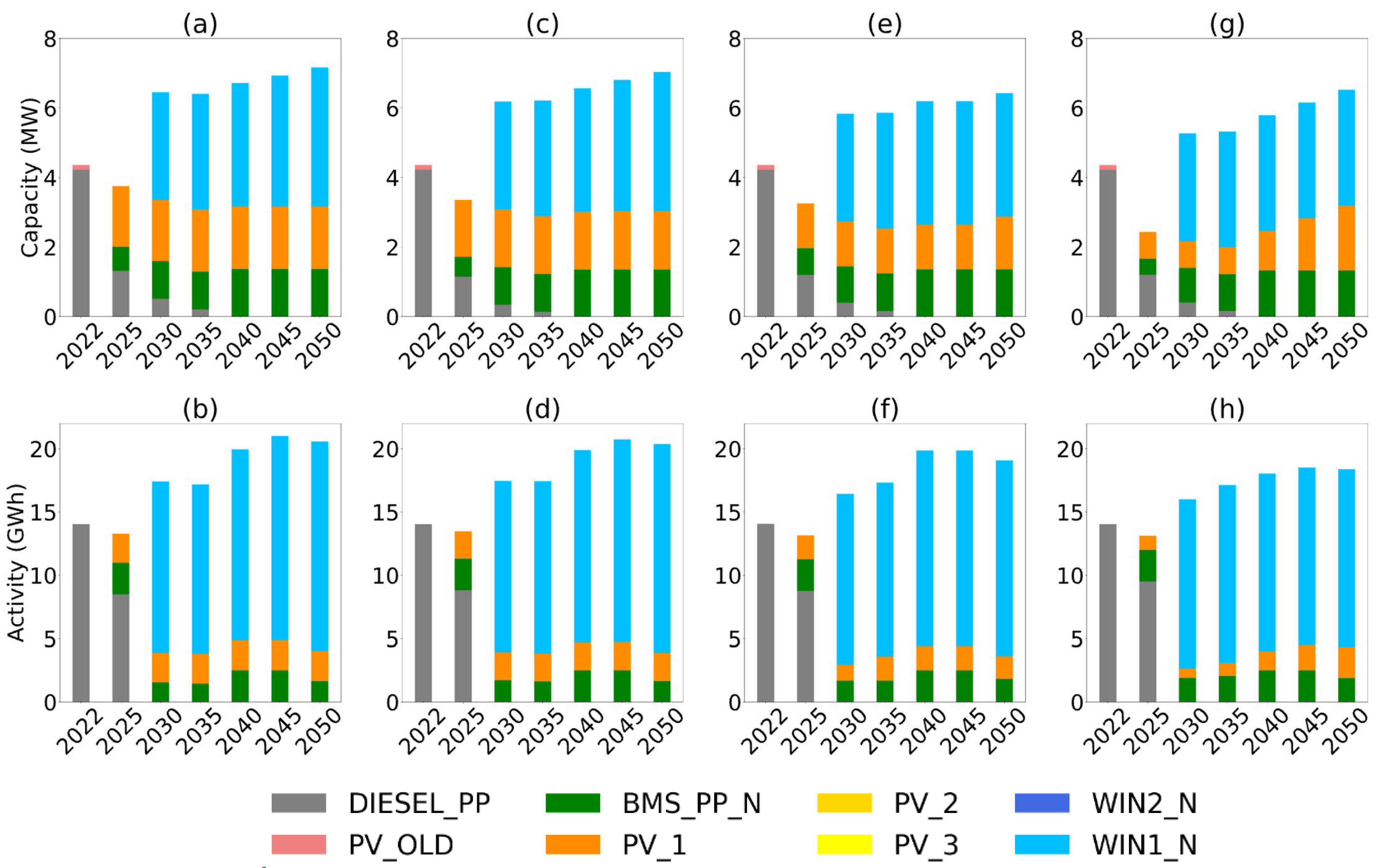
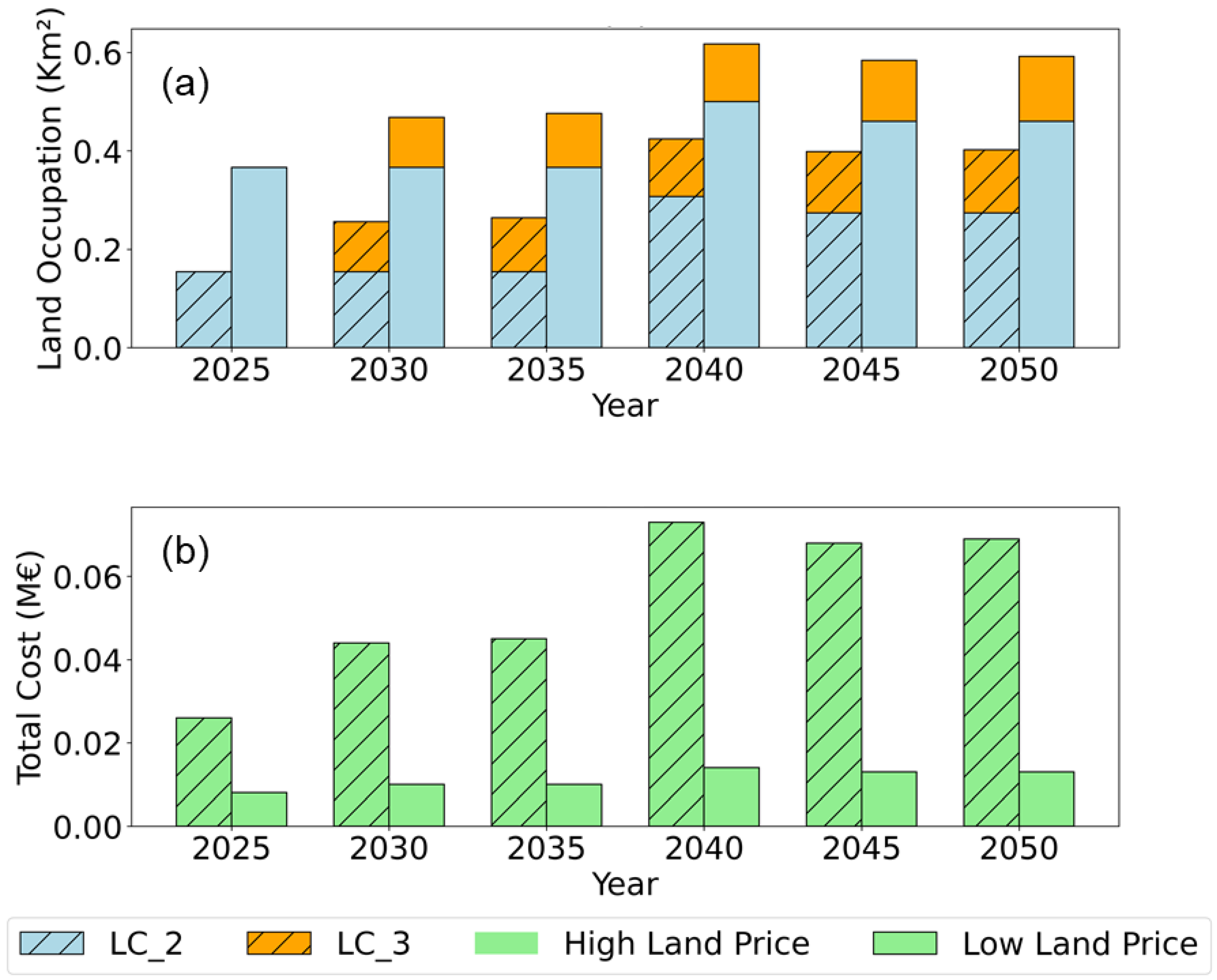
4.2. Energy Scenario Analysis

Energy scenarios, referring to optimized technological mix in terms of activity and capacity, then generating emissions and costs, are discussed here. Since the objective is to test how the land use module changes model outcome, the results are proposed for the two different model configurations. The land-explicit one is tested with a parametric analysis of the land price, making this last vary between the minimum and the maximum possible values. Due to the power sector-focused approach of this work, the main outcomes presented are the electricity generation (capacity and activity, Figure 8), the relative energy system cost differences, and the land consumption for the land-explicit modelling instance. Starting from the power sector configuration, in Figure 8, the capacity (MW) and the electricity generation (GWh) are presented. In all the configurations, differences in the outcomes are appreciable both in terms of absolute and relative amounts. Indeed, the scenarios differ for the total installed capacity and the generated electricity, but also in the way these amounts are obtained. First, it can be easily noticed (and confirmed by subsequent data analysis, not shown) that the traditional model and the low land price configuration do not present any differences, as expected, while the high land price instance has significative differences concerning the previous two. This is a symptom of a threshold phenomenon that changes model outcomes under a certain land price value.
Going into detail, the traditional TEMOA-Pantelleria and the low land price instances present a higher installed capacity concerning the high land price configuration. In the first two cases, the capacity of energy technologies starts at just under 2 MW in 2020 and shows a more than threefold increase to approximately 7 MW by 2050. The technology mix remains relatively stable, with wind technologies dominating the share, followed by solar and biomass, the last mostly covering the base load needs. Considering the activity, its level starts at around 15 GWh in 2020, increasing to nearly 23 GWh by 2050. This increase is justified by the increased electrification (mainly in the transport sector) caused by the decarbonization constraints to which the island is subjected. The proportions of each technology within the activity profile change slightly over time, with “WIN1_N” gaining a larger share, indicative of not only increased capacity but also high utilization rates. The most valuable outcomes visible from Figure 8 are related to the differences in the photovoltaic installations and the overall power production between the two previously described configurations.
In both the zero (or low) and high land price configurations, there is a growth in capacity over time, but the technology preferences differ. In the low/null land price case (a)/(c), there is a major reliance on solar technology (PV_1, the highest performing one), which suggests that larger, more land-intensive solar projects are feasible and economically viable due to lower land costs. Conversely, with a higher land price (e), there is a marked preference for wind systems, indicative of a strategy to maximize energy yield per unit of land area. In particular, the total difference in 2050 is 1.2 MW of installed capacity and around 2.2 GWh of electricity produced. This consumption gap is mainly driven by the commercial and residential sectors.
It must be specified that, in all the cases, the limitation caused by the land use constraint of Equation (19) does not influence the model outcome. This happens because the necessary capacity for the Pantelleria power sector is not occupying any land cluster at its maximum. Indeed, the model selects the highest performing technologies (WIN1_N, PV1_N) considering the limitation of the cluster these are installed in. This consideration is supported by Figure 9, which highlights the land cluster occupation and the land price costs in the two-model configuration.
In Figure 9a, the difference in land occupation by cluster in the two model configurations is shown. In both cases, the land cluster “LC_3” is the most consumed due to the installation of the solar technology “PV1_N”, reaching a maximum occupation of ~10% at low price and ~6% at low price in 2040. Even if LC_3 is the one with the highest absolute occupation, LC_2, due to its limited extension, is the one reaching the highest percentage of occupation. Indeed, in 2040, due to the installation of WIN1_N, LC_2 is occupied at 26% in both the configurations. These considerations are reflected in the cost, which notably shows higher values for the high price configuration. In this configuration, land rent price start from EUR 0.026 M in 2025, increasing and stabilizing around EUR 0.07 M from 2040 to the last year. In the low-price instance, these costs are much lower, reaching a maximum of EUR 0.014 M in 2040.

5. Discussion

The initial goal of this research was to quantify how much spatial information, as well as the consideration of regional characteristics, can improve planning solutions when integrated within an ESOM. This comprehensive review justifies three hypotheses regarding the impact of spatially explicit ESOMs: the influence of spatial resolution, land availability, and sectorial trade-offs. The objective was to obtain a modeling instance able to account for all these aspects, optimally allocating the new installation of renewable energy plants, accounting for local conditions such as cost of occupying land and factors affecting its availability. This research effectively demonstrates the feasibility and benefits of incorporating spatially explicit considerations into ESOMs using open source packages, highlighting the practicality and value of this approach. This integration not only enhances the realism and applicability of these models but also aligns with the pressing global shift toward sustainable and renewable energy sources. Also, by comparing traditional and spatially enhanced models, the study quantifies the added value brought by spatial planning and the influence of the new variable introduced in the model. While this approach does not represent a groundbreaking milestone in the field, it introduces an innovative methodology accompanied by certain limitations. As such, a critical discussion of this work is imperative.
Concerning the assessment phase, referring to the practice of gathering data about renewable energy potential of a region (both in terms of physical and administrative availability), this can be further divided in two subtopics: data gathering and elaboration. In terms of data gathering, the need for a unified tool to perform this kind of analysis is evident. The currently available literature still relies on many incompatible packages for this analysis, even if some exceptions are arising. For example, the GLAES framework for LE analysis [21] has found recent application in different studies [70]. In terms of the renewable energy potential assessment phase, there have been many valuable attempts ([28,39]), but a uniformly adopted methodology across studies is missing. In general, an interface to integrate spatial and temporal explicit data about VRESs is needed. Even if, as confirmed by Aryanpur et al. [20], the optimal choice of resolution is still dependent on model scope, the uncertainties inherent in the assessment phase predominantly stem from the analysis of land eligibility, complicated by ambiguous energy legislation. Notably, our approach did not consider buffer zones around any protected areas, a decision that potentially leads to an overestimation of available land. Further analysis (not detailed here) reveals that implementing buffer zones ranging from 25 to 200 m around these areas drastically affects land availability. In some clusters, this results in the complete unavailability of land, while in the most favorable scenarios, it causes a reduction of approximately 25%. Specifically, in the context of wind technology, the application of buffer zones rendered certain land clusters unsuitable, significantly altering the potential energy mix. This outcome underscores the necessity for more transparent and comprehensible landscape regulations. The challenge in setting fixed buffer values, as indicated by [77], further complicates this issue, necessitating a nuanced approach to landscape management in the context of renewable energy development.
Diving into the model’s integration, the first and primary challenge in implementing land use in an ESOM is the proliferation of energy technologies. This challenge arises due to the necessity of introducing, after the clustering, a multitude of technologies equivalent to the number of clusters employed. While this approach may find some applicability in constrained environments like the island of Pantelleria, its feasibility diminishes significantly in more expansive scenarios, such as national or European contexts. In this context, there is a need to find a trade-off between model accuracy and computational effort. Stolten et al. [28] highlight how this practice is strongly dependent on both spatial and temporal resolution and should be faced case by case. Despite the methodological issues, there is general knowledge that can be extracted from these results. The results indicate how the cost of land has a strong influence in limiting the land use intensive renewable energy sources, such as photovoltaic. The sensitivity analysis conducted according to Eurostat [109] suggests that economic factors, such as land prices, significantly influence technology selection and deployment strategies, leading to regional differentiation in the energy mix. According to this point, another remarkable limitation of this study is not considering the trade-offs and synergies concerning other land use-intensive sectors. For example, agrivoltaic is an innovative solution and further research is required estimate the actual benefits and their significance, especially about land type and soil conditions [38].

6. Conclusions

This study introduces a novel methodological framework for integrating spatial considerations within ESOMs. Thanks to a detailed literature review, this research emphasizes the importance of including land use aspects in energy planning, particularly in small, diverse geographical areas. This justifies the choice of Pantelleria Island as a case study. The review emphasizes the criticality of spatial resolution in ESOMs, the strategic allocation of space for renewable energy installations concerning land availability and optimal siting, and the sectorial trade-offs between energy production and land use. The methodology introduces a new and versatile framework for incorporating the three identified aspects into ESOMs. First, it involves collecting and converting a large amount of site-specific data into a format that can be interpreted by the model. Second, it entails integrating this data into an open source ESOM, TEMOA, introducing new parameters and modifying equations in the model. The results highlight the benefits of such analysis in model configuration, particularly due to the technological diversity revealed; future research should explore the scale up of this method on a broader spatial and technological scope. The findings underscore the crucial role of detailed territorial descriptions in the modeling phase, considering technological discretization, land pricing, and area availability. A conducted sensitivity analysis on land pricing reveals threshold phenomena within models that could significantly alter scenario outcomes. This research underscores the need for considering trade-offs within land use sectors, especially in relation to agriculture, carbon capture, and afforestation, which should gain more space in future ESOMs. This study’s primary limitations stem from the static nature of land prices over time and the inadequate modeling of land use sectors, which affects many ESOMs. Future research should focus on these areas, offering comprehensive sensitivity analyses on spatial resolution, land use constraints, and land prices to determine which factor is most influential. Integrating land use change emissions from renewables into ESOMs is also necessary. Overall, by introducing a new method that simplifies the inclusion of land use and its effect on carbon levels in ESOMs, this paper offers a valuable perspective on the role of land in achieving carbon neutrality.

Supplementary Materials

The Python scripts and other supporting information can be downloaded at: https://data.mendeley.com/preview/kp7hw83h92?a=47d02faa-9a33-4ff1-9703-6b432466ec6c (accessed on 30 December 2023).

Author Contributions

Conceptualization, D.M. and L.S.; methodology, D.M. and L.R.; software, D.M. and L.R.; validation, L.S.; formal analysis, D.M.; investigation, D.M. and L.S.; resources, L.S.; data curation, L.R.; writing—original draft preparation, D.M.; writing—review and editing, L.S. and L.R.; visualization, L.R.; supervision, D.M.; project administration, L.S.; funding acquisition, L.S. All authors have read and agreed to the published version of the manuscript.

Funding

This research received funding from the Italian Ministry of University and Research under the PNRR DM 352/ENI agreement.

Institutional Review Board Statement

Not applicable.

Informed Consent Statement

Not applicable.

Data Availability Statement

The Python scripts, the original data, and the excel sheets of the analyzed scenario, as well as other supporting information, can be downloaded from Supplementary Materials at https://data.mendeley.com/preview/kp7hw83h92?a=47d02faa-9a33-4ff1-9703-6b432466ec6c.

Acknowledgments

We thank Farzaneh Amir Kavei and Maria Elena Alfano for model database development, and Gianvito Colucci, Daniele Lerede and Matteo Nicoli for insightful discussion and brainstorming.

Conflicts of Interest

The authors declare no conflicts of interest.

Abbreviations

AcronymMeaning
AEPannual energy production
AHPanalytical hierarchy process
CFcapacity factor
CLCCorine land cover
DBSCANdensity-based spatial clustering of applications with noise
DEMdigital elevation model
ESOMsenergy system optimization models
GHIglobal horizontal irradiation
GISsgeographical information systems
GWAGlobal Wind Atlas
HDBSCANhierarchical density-based spatial clustering of applications with noise
IAMsintegrated assessment models
IQRinterquartile range
KmeansK-means clustering algorithm
LCOElevelized cost of electricity
LEland eligibility
LUIland use intensity
MILPmixed integer linear programming
MADMmulti-attribute decision making
O&Moperations and maintenance
PVphotovoltaic
PRperformance ratio
TEMOAtool for energy model optimization and analysis
VRESsvariable renewable energy sources
WDPAWorld Database of Protected Areas
WTwind turbines
WTGwind turbine generator

References

  1. Fawzy, S.; Osman, A.I.; Doran, J.; Rooney, D.W. Strategies for mitigation of climate change: A review. Environ. Chem. Lett. 2020, 18, 2069–2094. [Google Scholar] [CrossRef]
  2. VijayaVenkataRaman, S.; Iniyan, S.; Goic, R. A review of climate change, mitigation and adaptation. Renew. Sustain. Energy Rev. 2012, 16, 878–897. [Google Scholar] [CrossRef]
  3. Gabrielli, P.; Rosa, L.; Gazzani, M.; Meys, R.; Bardow, A.; Mazzotti, M.; Sansavini, G. Net-zero emissions chemical industry in a world of limited resources. One Earth 2023, 6, 682–704. [Google Scholar] [CrossRef]
  4. Martins, F.; Moura, P.; de Almeida, A.T. The Role of Electrification in the Decarbonization of the Energy Sector in Portugal. Energies 2022, 15, 1759. [Google Scholar] [CrossRef]
  5. International Renewable Energy Agency (IRENA). Electricity Storage and Renewables: Costs and Markets to 2030. 2017. Available online: https://www.irena.org/-/media/Files/IRENA/Agency/Publication/2017/Oct/IRENA_Electricity_Storage_Costs_2017.pdf (accessed on 26 June 2023).
  6. Lovering, J.; Swain, M.; Blomqvist, L.; Hernandez, R.R. Land-use intensity of electricity production and tomorrow’s energy landscape. PLoS ONE 2022, 17, e0270155. [Google Scholar] [CrossRef]
  7. Merfort, L.; Bauer, N.; Humpenöder, F.; Klein, D.; Strefler, J.; Popp, A.; Luderer, G.; Kriegler, E. State of global land regulation inadequate to control biofuel land-use-Chang. emissions. Nat. Clim. Chang. 2023, 13, 610–612. [Google Scholar] [CrossRef]
  8. Van de Ven, D.-J.; Capellan-Peréz, I.; Arto, I.; Cazcarro, I.; de Castro, C.; Patel, P.; Gonzalez-Eguino, M. The potential land requirements and related land use change emissions of solar energy. Sci. Rep. 2021, 11, 2907. [Google Scholar] [CrossRef]
  9. Chang, M.; Thellufsen, J.Z.; Zakeri, B.; Pickering, B.; Pfenninger, S.; Lund, H.; Østergaard, P.A. Trends in tools and approaches for modelling the energy transition. Appl. Energy 2021, 290, 116731. [Google Scholar] [CrossRef]
  10. Prina, M.G.; Manzolini, G.; Moser, D.; Nastasi, B.; Sparber, W. Classification and challenges of bottom-up energy system models—A review. Renew. Sustain. Energy Rev. 2020, 129, 109917. [Google Scholar] [CrossRef]
  11. Loulou, R.; Goldstein, G.; Kanudia, A.; Lettila, A.; Remme, U. Documentation for the TIMES Model: Part I. 2016. Available online: https://iea-etsap.org/docs/Documentation_for_the_TIMES_Model-Part-I_July-2016.pdf (accessed on 17 October 2022).
  12. Lerede, D.; Bustreo, C.; Gracceva, F.; Lechón, Y.; Savoldi, L. Analysis of the Effects of Electrification of the Road Transport Sector on the Possible Penetration of Nuclear Fusion in the Long-Term European Energy Mix. Energies 2020, 13, 3634. [Google Scholar] [CrossRef]
  13. Lerede, D.; Bustreo, C.; Gracceva, F.; Saccone, M.; Savoldi, L. Techno-economic and environmental characterization of industrial technologies for transparent bottom-up energy modeling. Renew. Sustain. Energy Rev. 2021, 140, 110742. [Google Scholar] [CrossRef]
  14. Balbo, A.; Colucci, G.; Nicoli, M.; Savoldi, L. Exploring the Role of Hydrogen to Achieve the Italian Decarbonization Targets Using an Open-Source Energy System Optimization Model. 2023, pp. 89–100. Available online: https://publications.waset.org/10013040/exploring-the-role-of-hydrogen-to-achieve-the-italian-decarbonization-targets-using-an-open-source-energy-system-optimization-model (accessed on 25 April 2023).
  15. Limpens, G.; Jeanmart, H.; Maréchal, F. Belgian Energy Transition: What Are the Options? Energies 2020, 13, 261. [Google Scholar] [CrossRef]
  16. Eshraghi, H.; de Queiroz, A.R.; DeCarolis, J.F. US Energy-Related Greenhouse Gas Emissions in the Absence of Federal Climate Policy. Environ. Sci. Technol. 2018, 52, 9595–9604. [Google Scholar] [CrossRef] [PubMed]
  17. Barnes, T.; Shivakumar, A.; Brinkerink, M.; Niet, T. OSeMOSYS Global, an open-source, open data global electricity system model generator. Sci. Data 2022, 9, 1–13. [Google Scholar] [CrossRef]
  18. Gago Da Camara Simoes, S.; Nijs, W.; Ruiz Castello, P.; Sgobbi, A.; Radu, D.; Bolat, P.; Thiel, C.; Peteves, E. The JRC-EU-TIMES Model—Assessing the Long-Term Role of the SET Plan Energy Technologies; Publications Office of the European Union: Luxembourg, 2013. [Google Scholar] [CrossRef]
  19. Lerede, D.; Nicoli, M.; Savoldi, L.; Trotta, A. Analysis of the possible contribution of different nuclear fusion technologies to the global energy transition. Energy Strat. Rev. 2023, 49, 101144. [Google Scholar] [CrossRef]
  20. Aryanpur, V.; O’Gallachoir, B.; Dai, H.; Chen, W.; Glynn, J. A review of spatial resolution and regionalisation in national-scale energy systems optimisation models. Energy Strat. Rev. 2021, 37, 100702. [Google Scholar] [CrossRef]
  21. Ryberg, D.S.; Robinius, M.; Stolten, D. Evaluating Land Eligibility Constraints of Renewable Energy Sources in Europe. Energies 2018, 11, 1246. [Google Scholar] [CrossRef]
  22. Risch, S.; Maier, R.; Du, J.; Pflugradt, N.; Stenzel, P.; Kotzur, L.; Stolten, D. Potentials of Renewable Energy Sources in Germany and the Influence of Land Use Datasets. Energies 2022, 15, 5536. [Google Scholar] [CrossRef]
  23. Ramos, E.P.; Sridharan, V.; Alfstad, T.; Niet, T.; Shivakumar, A.; Howells, M.I.; Rogner, H.; Gardumi, F. Climate, Land, Energy and Water systems interactions—From key concepts to model implementation with OSeMOSYS. Environ. Sci. Policy 2022, 136, 696–716. [Google Scholar] [CrossRef]
  24. Lamhamedi, B.E.H.; de Vries, W.T. An Exploration of the Land–(Renewable) Energy Nexus. Land 2022, 11, 767. [Google Scholar] [CrossRef]
  25. Chen, Y.-K.; Kirkerud, J.G.; Bolkesjø, T.F. Balancing GHG mitigation and land-use conflicts: Alternative Northern European energy system scenarios. Appl. Energy 2022, 310, 118557. [Google Scholar] [CrossRef]
  26. Bacca, E.J.M.; Stevanović, M.; Bodirsky, B.L.; Karstens, K.; Chen, D.M.-C.; Leip, D.; Müller, C.; Minoli, S.; Heinke, J.; Jägermeyr, J.; et al. Uncertainty in land-use adaptation persists despite crop model projections showing lower impacts under high warming. Commun. Earth Environ. 2023, 4, 284. [Google Scholar] [CrossRef]
  27. Moksnes, N.; Howells, M.; Usher, W. Increasing spatial and temporal resolution in energy system optimisation model—The case of Kenya. Energy Strat. Rev. 2024, 51, 101263. [Google Scholar] [CrossRef]
  28. Patil, S.; Kotzur, L.; Stolten, D. Advanced Spatial and Technological Aggregation Scheme for Energy System Models. Energies 2022, 15, 9517. [Google Scholar] [CrossRef]
  29. Resch, B.; Sagl, G.; Törnros, T.; Bachmaier, A.; Eggers, J.-B.; Herkel, S.; Narmsara, S.; Gündra, H. GIS-Based Planning and Modeling for Renewable Energy: Challenges and Future Research Avenues. ISPRS Int. J. Geo-Inf. 2014, 3, 662–692. [Google Scholar] [CrossRef]
  30. Maclaurin, G.; Grue, N.; Lopez, A.; Heimiller, D.; Rossol, M.; Buster, G.; Williams, T. The Renewable Energy Potential (reV) Model: A Geospatial Platform for Technical Potential and Supply Curve Modeling. 2021. Available online: https://www.nrel.gov/gis/renewable-energy-potential.html (accessed on 1 February 2023).
  31. Wang, N.; Verzijlbergh, R.A.; Heijnen, P.W.; Herder, P.M. A spatially explicit planning approach for power systems with a high share of renewable energy sources. Appl. Energy 2019, 260, 114233. [Google Scholar] [CrossRef]
  32. Martínez-Gordón, R.; Morales-España, G.; Sijm, J.; Faaij, A. A review of the role of spatial resolution in energy systems modelling: Lessons learned and applicability to the North Sea region. Renew. Sustain. Energy Rev. 2021, 141, 110857. [Google Scholar] [CrossRef]
  33. Yliruka, M.I.; Moret, S.; Jalil-Vega, F.; Hawkes, A.D.; Shah, N. The Trade-Off between Spatial Resolution and Uncertainty in Energy System Modelling. Comput. Aided Chem. Eng. 2022, 49, 2035–2040. [Google Scholar] [CrossRef]
  34. Archer, C.L.; Jacobson, M.Z. Supplying Baseload Power and Reducing Transmission Requirements by Interconnecting Wind Farms. J. Appl. Meteorol. Clim. 2007, 46, 1701–1717. [Google Scholar] [CrossRef]
  35. Frysztacki, M.M.; Hörsch, J.; Hagenmeyer, V.; Brown, T. The strong effect of network resolution on electricity system models with high shares of wind and solar. Appl. Energy 2021, 291, 116726. [Google Scholar] [CrossRef]
  36. Frysztacki, M.M.; Hagenmeyer, V.; Brown, T. Inverse methods: How feasible are spatially low-resolved capacity expansion modelling results when disaggregated at high spatial resolution? Energy 2023, 281, 128133. [Google Scholar] [CrossRef]
  37. McKinsey. Land: A Crucial Resource for Europe’s Energy Transition. Available online: https://www.mckinsey.com/industries/electric-power-and-natural-gas/our-insights/land-a-crucial-resource-for-the-energy-transition (accessed on 8 November 2023).
  38. Stucchi, L.; Aiello, M.; Gargiulo, A.; Brovelli, M.A. Copernicus and the energy challenge. ISPRS Int. Arch. Photogramm. Remote. Sens. Spat. Inf. Sci. 2021, XLVI-4/W2, 189–196. [Google Scholar] [CrossRef]
  39. Hofmann, F.; Hampp, J.; Neumann, F.; Brown, T.; Hörsch, J. atlite: A Lightweight Python Package for Calculating Renewable Power Potentials and Time Series. J. Open Source Softw. 2021, 6, 3294. [Google Scholar] [CrossRef]
  40. Dominguez, O.D.M.; Kasmaei, M.P.; Lavorato, M.; Mantovani, J.R.S. Optimal siting and sizing of renewable energy sources, storage devices, and reactive support devices to obtain a sustainable electrical distribution systems. Energy Syst. 2018, 9, 529–550. [Google Scholar] [CrossRef]
  41. Attaullah; Ashraf, S.; Rehman, N.; Khan, A.; Naeem, M.; Park, C. A wind power plant site selection algorithm based on q-rung orthopair hesitant fuzzy rough Einstein aggregation information. Sci. Rep. 2022, 12, 5443. [Google Scholar] [CrossRef]
  42. Zanakis, S.H.; Solomon, A.; Wishart, N.; Dublish, S. Multi-attribute decision making: A simulation comparison of select methods. Eur. J. Oper. Res. 1998, 7, 507–529. [Google Scholar] [CrossRef]
  43. Türk, S.; Koç, A.; Şahin, G. Multi-criteria of PV solar site selection problem using GIS-intuitionistic fuzzy based approach in Erzurum province/Turkey. Sci. Rep. 2021, 11, 5034. [Google Scholar] [CrossRef] [PubMed]
  44. Topuz, M.; Deniz, M. Application of GIS and AHP for land use suitability analysis: Case of Demirci district (Turkey). Humanit. Soc. Sci. Commun. 2023, 10, 115. [Google Scholar] [CrossRef]
  45. Jones, S.M.; Smith, A.C.; Leach, N.; Henrys, P.; Atkinson, P.M.; Harrison, P.A. Pathways to achieving nature-positive and carbon–neutral land use and food systems in Wales. Reg. Environ. Chang. 2023, 23, 37. [Google Scholar] [CrossRef]
  46. Caldera, U.; Breyer, C. Afforesting arid land with renewable electricity and desalination to mitigate climate change. Nat. Sustain. 2023, 6, 526–538. [Google Scholar] [CrossRef]
  47. Adeh, E.H.; Good, S.P.; Calaf, M.; Higgins, C.W. Solar PV Power Potential is Greatest Over Croplands. Sci. Rep. 2019, 9, 11442. [Google Scholar] [CrossRef] [PubMed]
  48. Niet, T.; Fraser, S.; Arianpoo, N.; Kuling, K.; Wright, A.; Wright, A.S. Embedding the United Nations Sustainable Development Goals into Systems Analysis—Expanding the Food-Energy-Water Nexus. 2020. Available online: https://assets.researchsquare.com/files/rs-52249/v1_stamped.pdf?c=1597093325 (accessed on 30 December 2023).
  49. Zhou, J.; Ding, Q.; Zou, Z.; Deng, J.; Xu, C.; Yang, W. Land suitability evaluation of large-scale photovoltaic plants using structural equation models. Resour. Conserv. Recycl. 2023, 198, 107179. [Google Scholar] [CrossRef]
  50. Temoa Project. Temoa Project Documentation. Available online: https://temoacloud.com/temoaproject/index.html (accessed on 12 July 2023).
  51. Loulou, R.; Lehtilä, A.; Kanudia, A.; Remme, U.; Goldstein, G. Documentation for the TIMES Model: Part II. 2016. Available online: https://iea-etsap.org/docs/Documentation_for_the_TIMES_Model-Part-II_July-2016.pdf (accessed on 30 December 2023).
  52. MESSAGEix-GLOBIOM Documentation—Message_Doc 2020 Documentation. Available online: https://docs.messageix.org/projects/global/en/latest/ (accessed on 6 November 2023).
  53. Hainoun, A.; Aldin, M.S.; Almoustafa, S. Formulating an optimal long-term energy supply strategy for Syria using MESSAGE model. Energy Policy 2010, 38, 1701–1714. [Google Scholar] [CrossRef]
  54. Howells, M.; Rogner, H.; Strachan, N.; Heaps, C.; Huntington, H.; Kypreos, S.; Hughes, A.; Silveira, S.; DeCarolis, J.; Bazillian, M.; et al. OSeMOSYS: The Open Source Energy Modeling System: An introduction to its ethos, structure and development. Energy Policy 2011, 39, 5850–5870. [Google Scholar] [CrossRef]
  55. Plazas-Niño, F.; Yeganyan, R.; Cannone, C.; Howells, M.; Quirós-Tortós, J. Informing sustainable energy policy in developing countries: An assessment of decarbonization pathways in Colombia using open energy system optimization modelling. Energy Strat. Rev. 2023, 50, 2211–2467. [Google Scholar] [CrossRef]
  56. Nicoli, M.; Gracceva, F.; Lerede, D.; Savoldi, L. Can We Rely on Open-Source Energy System Optimization Models? The TEMOA-Italy Case Study. Energies 2022, 15, 6505. [Google Scholar] [CrossRef]
  57. GitHub. TemoaProject GitHub—TemoaProject/Temoa. Available online: https://github.com/TemoaProject/temoa (accessed on 11 February 2023).
  58. Nicoli, M. A TIMES-like Open-Source Model for the Italian Energy System; Politecnico di Torino: Turin, Italy, 2021; Available online: https://webthesis.biblio.polito.it/18850/ (accessed on 5 July 2022).
  59. Pantelleria—Clean Energy for EU Islands. Available online: https://energy.ec.europa.eu/topics/markets-and-consumers/clean-energy-eu-islands_en (accessed on 14 June 2023).
  60. Comune di Pantelleria. Available online: https://www.comunepantelleria.it/ (accessed on 1 February 2023).
  61. Aeolian. Available online: https://atlanteeolico.rse-web.it/ (accessed on 8 November 2023).
  62. Moscoloni, C.; Zarra, F.; Novo, R.; Giglio, E.; Vargiu, A.; Mutani, G.; Bracco, G.; Mattiazzo, G. Wind Turbines and Rooftop Photovoltaic Technical Potential Assessment: Application to Sicilian Minor Islands. Energies 2022, 15, 5548. [Google Scholar] [CrossRef]
  63. Novo, R.; Minuto, F.D.; Bracco, G.; Mattiazzo, G.; Borchiellini, R.; Lanzini, A. Supporting Decarbonization Strategies of Local Energy Systems by De-Risking Investments in Renewables: A Case Study on Pantelleria Island. Energies 2022, 15, 1103. [Google Scholar] [CrossRef]
  64. Alfano, M.E. Modeling the Energy and the Water Systems in an Open-Access Energy System Optimization Model: The Pantelleria Case Study; Politecnico di Torino: Turin, Italy, 2022; Available online: https://webthesis.biblio.polito.it/24982/ (accessed on 19 January 2023).
  65. Isola di Pantelleria Verso 100% Rinnovabile—Scenari per Nuovi Paesaggi Dell’energia. Available online: https://it.readkong.com/page/isola-di-pantelleria-verso-100-rinnovabile-scenari-per-5867995 (accessed on 18 November 2023).
  66. Ansari, M.Y.; Ahmad, A.; Khan, S.S.; Bhushan, G. Mainuddin Spatiotemporal clustering: A review. Artif. Intell. Rev. 2020, 53, 2381–2423. [Google Scholar] [CrossRef]
  67. Balkovič, J.; van der Velde, M.; Schmid, E.; Skalský, R.; Khabarov, N.; Obersteiner, M.; Stürmer, B.; Xiong, W. Pan-European crop modelling with EPIC: Implementation, up-scaling and regional crop yield validation. Agric. Syst. 2013, 120, 61–75. [Google Scholar] [CrossRef]
  68. Joint Research Centre. European Meteorological Derived High Resolution RES Generation Time Series for Present and Future Scenarios (EMHIRES). 2021. Available online: https://data.jrc.ec.europa.eu/collection/id-0055#:~:text=EMHIRES (accessed on 12 July 2023).
  69. McKenna, R.; Hollnaicher, S.; Fichtner, W. Cost-potential curves for onshore wind energy: A high-resolution analysis for Germany. Appl. Energy 2013, 115, 103–115. [Google Scholar] [CrossRef]
  70. Ryberg, D.S.; Tulemat, Z.; Stolten, D.; Robinius, M. Uniformly constrained land eligibility for onshore European wind power. Renew. Energy 2020, 146, 921–931. [Google Scholar] [CrossRef]
  71. McKenna, R.; Pfenninger, S.; Heinrichs, H.; Schmidt, J.; Staffell, I.; Bauer, C.; Gruber, K.; Hahmann, A.N.; Jansen, M.; Klingler, M.; et al. High-resolution large-scale onshore wind energy assessments: A review of potential definitions, methodologies and future research needs. Renew. Energy 2021, 182, 659–684. [Google Scholar] [CrossRef]
  72. Klok, C.; Kirkels, A.; Alkemade, F. Impacts, procedural processes, and local context: Rethinking the social acceptance of wind energy projects in the Netherlands. Energy Res. Soc. Sci. 2023, 99, 2214–6296. [Google Scholar] [CrossRef]
  73. Rete Natura 2000—S.I.T.R—Sistema Informativo Territoriale Regionale. Available online: https://www.sitr.regione.sicilia.it/download/tematismi/rete-natura-2000/ (accessed on 1 February 2023).
  74. Explore the World’s Protected Areas. Available online: https://www.protectedplanet.net/en/thematic-areas/wdpa?tab=WDPA (accessed on 9 November 2023).
  75. OpenStreetMap. Available online: https://www.openstreetmap.org/#map=7/42.727/12.371 (accessed on 9 November 2023).
  76. Sousa, A. The Thematic Accuracy of Corine Land cover 2000 Assessment Using LUCAS (Land Use/Cover Area Frame Statistical Survey). Available online: https://www.eea.europa.eu/publications/technical_report_2006_7 (accessed on 9 February 2024).
  77. Comune di Pantelleria Piano D’azione Per L’energia Sostenibile. 2015. Available online: www.ambienteitalia.it (accessed on 30 October 2023).
  78. Lindberg, F.; Grimmond, C.; Gabey, A.; Huang, B.; Kent, C.W.; Sun, T.; Theeuwes, N.E.; Järvi, L.; Ward, H.C.; Capel-Timms, I.; et al. Urban Multi-scale Environmental Predictor (UMEP): An integrated tool for city-based climate services. Environ. Model. Softw. 2018, 99, 70–87. [Google Scholar] [CrossRef]
  79. Tarquini, S.; Vinci, S.; Favalli, M.; Doumaz, F.; Fornaciai, A.; Nannipieri, L. Release of a 10-m-resolution DEM for the Italian territory: Comparison with global-coverage DEMs and anaglyph-mode exploration via the web. Comput. Geosci. 2012, 38, 168–170. [Google Scholar] [CrossRef]
  80. Rete Natura 2000—Ministero dell’Ambiente e della Sicurezza Energetica. Available online: https://www.mase.gov.it/pagina/rete-natura-2000 (accessed on 9 November 2023).
  81. Elkadeem, M.R.; Younes, A.; Mazzeo, D.; Jurasz, J.; Campana, P.E.; Sharshir, S.W.; Alaam, M.A. Geospatial-assisted multi-criterion analysis of solar and wind power geographical-technical-economic potential assessment. Appl. Energy 2022, 322, 119532. [Google Scholar] [CrossRef]
  82. Ramon, J.; Lledó, L.; Pérez-Zanón, N.; Soret, A.; Doblas-Reyes, F.J. The Tall Tower Dataset: A unique initiative to boost wind energy research. Earth Syst. Sci. Data 2020, 12, 429–439. [Google Scholar] [CrossRef]
  83. Dunn, R.J.H.; Willett, K.M.; Thorne, P.W.; Woolley, E.V.; Durre, I.; Dai, A.; Parker, D.E.; Vose, R.S. HadISD: A quality-controlled global synoptic report database for selected variables at long-term stations from 1973–2011. Clim. Past 2012, 8, 1649–1679. [Google Scholar] [CrossRef]
  84. Bell, B.; Hersbach, H.; Simmons, A.; Berrisford, P.; Dahlgren, P.; Horányi, A.; Muñoz-Sabater, J.; Nicolas, J.; Radu, R.; Schepers, D.; et al. The ERA5 global reanalysis: Preliminary extension to 1950. Q. J. R. Meteorol. Soc. 2021, 147, 4186–4227. [Google Scholar] [CrossRef]
  85. MERRA-2. Available online: https://gmao.gsfc.nasa.gov/reanalysis/MERRA-2/ (accessed on 9 November 2023).
  86. HelioClim-3 Monthly Irradiation GHI—Data Europa EU. Available online: https://data.europa.eu/data/datasets/7237e78b-b12b-4fdb-85fb-33e9fe0c6994?locale=it (accessed on 9 November 2023).
  87. CMIP5—Home—ESGF-CoG. Available online: https://esgf-node.llnl.gov/projects/cmip5/ (accessed on 9 November 2023).
  88. EURO-CORDEX. Available online: https://www.euro-cordex.net/ (accessed on 9 November 2023).
  89. New European Wind Atlas. Available online: https://www.neweuropeanwindatlas.eu/ (accessed on 9 November 2023).
  90. Global Wind Atlas. Available online: https://globalwindatlas.info/en (accessed on 9 November 2023).
  91. Global Solar Atlas. Available online: https://globalsolaratlas.info/map (accessed on 9 November 2023).
  92. Solargis. Solar Irradiance Data. Available online: https://solargis.com/ (accessed on 9 November 2023).
  93. Home—Dutch Offshore Wind Atlas. Available online: https://www.dutchoffshorewindatlas.nl/ (accessed on 9 November 2023).
  94. UL Solutions. Windographer—Wind Data Analytics and Visualization Solution. Available online: https://www.ul.com/software/windographer-wind-data-analytics-and-visualization-solution (accessed on 9 November 2023).
  95. Mesonet—Home. Available online: https://mesonet.org/ (accessed on 9 November 2023).
  96. McCutchan, M.H.; Fox, D.G.; McCutchan, M.H.; Fox, D.G. Effect of Elevation and Aspect on Wind, Temperatme and Humidity. J. Appl. Meteorol. Climatol. 1986, 25, 1996–2013. [Google Scholar] [CrossRef]
  97. Chen, N. Scale problem: Influence of grid spacing of digital elevation model on computed slope and shielded extra-terrestrial solar radiation. Front. Earth Sci. 2019, 14, 171–187. [Google Scholar] [CrossRef]
  98. Šúri, M.; Hofierka, J. A New GIS-based Solar Radiation Model and Its Application to Photovoltaic Assessments. Trans. GIS 2004, 8, 175–190. [Google Scholar] [CrossRef]
  99. ArcGIS. Accesso di Accesso. Available online: https://www.arcgis.com/index.html (accessed on 9 November 2023).
  100. ArcGIS Pro. An overview of the Solar Radiation toolset—Documentation. Available online: https://pro.arcgis.com/en/pro-app/latest/tool-reference/spatial-analyst/an-overview-of-the-solar-radiation-tools.htm (accessed on 9 November 2023).
  101. Kausika, B.B.; van Sark, W.G.J.H.M. Calibration and Validation of ArcGIS Solar Radiation Tool for Photovoltaic Potential Determination in the Netherlands. Energies 2021, 14, 1865. [Google Scholar] [CrossRef]
  102. Pintor, B.H.; Sola, E.F.; Teves, J.; Inocencio, L.C.; Ang, M.R.C. Solar Energy Resource Assessment Using R.SUN In GRASS GIS And Site Suitability Analysis Using AHP For Groundmounted Solar Photovoltaic (PV) Farm in The Central Luzon Region (Region 3), Philippines. Free. Open Source Softw. Geospat. FOSS4G Conf. Proc. 2018, 15, 3. [Google Scholar] [CrossRef]
  103. Gašparović, I.; Gašparović, M.; Medak, D. Determining and analysing solar irradiation based on freely available data: A case study from Croatia. Environ. Dev. 2018, 26, 55–67. [Google Scholar] [CrossRef]
  104. El Chaar, L.; Lamont, L.A.; El Zein, N. Review of photovoltaic technologies. Renew. Sustain. Energy Rev. 2011, 15, 2165–2175. [Google Scholar] [CrossRef]
  105. Analysis of Utility Scale Wind and Solar Plant Performance in South Africa Relative to Daily Electricity Demand. Available online: https://www.researchgate.net/publication/321192910_Analysis_of_utility_scale_wind_and_solar_plant_performance_in_South_Africa_relative_to_daily_electricity_demand (accessed on 9 November 2023).
  106. Benvenuti a Wind-Turbine-Models. Available online: https://it.wind-turbine-models.com/ (accessed on 10 November 2023).
  107. Peterson, E.W.; Hennessey, J., Jr. On the Use of Power Laws for Estimates of Wind Power Potential. J. Appl. Meteorol. Climatol. 1978, 17, 390–394. [Google Scholar] [CrossRef]
  108. IRENA. Renewable Power Generation Costs in 2021, International Renewable Energy Agency, Abu Dhabi; International Renewable Energy Agency: Masdar City, United Arab Emirates, 2022; ISBN 978-92-9260-452-3. Available online: https://www.irena.org/-/media/Files/IRENA/Agency/Publication/2018/Jan/IRENA_2017_Power_Costs_2018.pdf (accessed on 10 November 2023).
  109. Eurostat Data Browser Yearly Land Rent Price for a Year. Available online: https://ec.europa.eu/eurostat/databrowser/view/APRI_LRNT__custom_5264437/bookmark/table?lang=en&bookmarkId=0e5713d6-6cad-4033-b9ac-e09b5270c489 (accessed on 10 November 2023).
  110. Austin, K.G.; Baker, J.S.; Sohngen, B.L.; Wade, C.M.; Daigneault, A.; Ohrel, S.B.; Ragnauth, S.; Bean, A. The economic costs of planting, preserving, and managing the world’s forests to mitigate climate change. Nat. Commun. 2020, 11, 5946. [Google Scholar] [CrossRef] [PubMed]
  111. Terna Spa. Econnextion: La Mappa Delle Connessioni Rinnovabili. Available online: https://www.terna.it/it/sistema-elettrico/rete/econnextion (accessed on 10 November 2023).
  112. Temoa Project. Temoa Project Documentation—Objective Function. Available online: https://temoacloud.com/temoaproject/Documentation.html#objective-function (accessed on 22 March 2023).
  113. Wind Costs. Available online: https://www.irena.org/Data/View-data-by-topic/Costs/Wind-Costs (accessed on 10 November 2023).
  114. Hughes, M.; Kelbaugh, M.; Campbell, V.; Reilly, E.; Agarwala, S.; Wilt, M.; Badger, A.; Fuller, E.; Ponzo, D.; Arevalo, X.C.; et al. System Integration with Multiscale Networks (Simon): A Modular Framework for Resource Management Models. In Proceedings of the 2020 Winter Simulation Conference (WSC), Orlando, FL, USA, 14–18 December 2020; pp. 656–667. [Google Scholar] [CrossRef]
  115. Campello, R.J.G.B.; Moulavi, D.; Sander, J. Density-based clustering based on hierarchical density estimates. In Lecture Notes in Computer Science (Including Subseries Lecture Notes in Artificial Intelligence and Lecture Notes in Bioinformatics); Springer: Berlin/Heidelberg, Germany, 2003; Volume 7819, LNAI, No. PART 2; pp. 160–172. [Google Scholar]
  116. Mannor, S.; Jin, X.; Han, J.; Zhang, X. K-Means Clustering. In Encyclopedia of Machine Learning; Springer: Boston, MA, USA, 2011; pp. 563–564. [Google Scholar] [CrossRef]
  117. Ester, M.; Kriegel, H.-P.; Sander, J.; Xu, X. A Density-Based Algorithm for Discovering Clusters in Large Spatial Databases with Noise. 1996. Available online: www.aaai.org (accessed on 13 November 2023).
  118. Wang, J.-F.; Stein, A.; Gao, B.-B.; Ge, Y. A review of spatial sampling. Spat. Stat. 2012, 2, 1–14. [Google Scholar] [CrossRef]
  119. Guo, G.; Wang, H.; Bell, D.; Bi, Y.; Greer, K. KNN model-based approach in classification. In Lecture Notes in Computer Science (Including Subseries Lecture Notes in Artificial Intelligence and Lecture Notes in Bioinformatics); Springer: Berlin/Heidelberg, Germany, 2003; Volume 2888, pp. 986–996. [Google Scholar]
  120. Rousseeuw, P.J. Silhouettes: A graphical aid to the interpretation and validation of cluster analysis. J. Comput. Appl. Math. 1987, 20, 53–65. [Google Scholar] [CrossRef]
Figure 1. Workflow of the methodology adopted in the present study.
Sustainability 16 01644 g001
Figure 2. Visualization of Pantelleria island’s energy availability. (a) Annual global irradiance; (b) wind mean velocity.
Sustainability 16 01644 g002
Figure 3. Land eligibility analysis for Pantelleria Island. (ac) represent the constraint for photovoltaic installations while (df) are the ones for wind. (a,d) are anthropic exclusion. (b,e) are constant due to natural habitat and landscape heritage laws. (c,f) represent limitations associated with environmental reasons. Dark blue represents unavailable areas.
Sustainability 16 01644 g003
Figure 4. Photovoltaic capacity factor by seasonal day (a) and peak (b) time slices.
Sustainability 16 01644 g004
Figure 5. Wind capacity factor by time slice and height. Average value, standard deviation, minimum and maximum values.
Sustainability 16 01644 g005
Figure 6. Results of clustering with different algorithms. (a) HDBSCAN, (b) Kmeans, and (c) DBSCAN.
Sustainability 16 01644 g006
Figure 7. Variability in capacity factor across different time slices: Figure (a) illustrates the case of PV with three distinct technological clusters and their average. Similarly, (b) show the WT case, with two distinct clusters and their average.
Sustainability 16 01644 g007
Figure 8. Power sector capacity and activity for traditional modelling instance and land-specific modeling instance. Subplot (a,b) represents the traditional TEMOA modeling instance, while (c,d) the land-explicit one in the low land price case, (e,f) the intermediate and (g,h) the high price configuration.
Sustainability 16 01644 g008
Figure 9. (a) Land occupation by cluster. (b) Total cost of land for different land price scenarios. Dashed columns represent the high-priced scenario, and blank columns represent the low-priced scenario.
Sustainability 16 01644 g009
Table 1. Review of mainland eligibility analysis found in the literature.
AdministrativeTechnicalEconomicSocialYearSource
vv 2014[69]
vvvv2018[21]
vvv 2020[31]
vvvv2020[70]
vvvv2021[39]
vv 2022[62]
vvvv2022[71]
vvvv2023[72]
Table 2. Constraints for the land eligibility analysis. The exclusion rule for distance is derived from Italian regulation summarized in the Pantelleria Energy Plan [77].
AreaConstraintExclusion RuleSource
Environmental/technicalWind speedBelow 4.5 m/sRSE [61]
IrradianceBelow 3.0 kWh/m2 dayUMEP ERA 5 [78]
Slope≥15%TinItaly [79]
Permanent cropsInsideCLC [76]
Water bodiesInside-
RocksInside-
CoastInside-
Administrative/habitatNatural habitatsInsideNatura 2000 [80]
Bird areasInside-
BiospheresInsideWDPA [74]
Protected landscape1000 m-
ReservesInside-
ParksInside-
Monuments1000 m-
Hydrological riskInside-
AnthropicRoad distance100 mOpenStreetMap [75]
Urban settlement200 m-
Industrial sites200 m-
Airport1500 m (wind only)-
Recreational areas200 m-
Table 4. Main characteristics of the wind turbine models used for the producibility calculation. For each turbine, data were obtained from the online wind turbine model repository [106].
Reference Height [m]WTG ModelNominal Power [MW]Rotor Diameter [m]Hub Height [m]
50 mRiva Calzoni 500.540.55450
75 mLeitwind LTW90-9500.959080
100 mVestas V117 34503.4511791
125 mNREL_6MW_RTW6128119
Table 5. Performance of the three different clustering algorithms.
MethodSilhouette ScoreTime (Seconds)Memory (MB)
HDBSCAN0.52717292246
K-means0.8270.3690.224
DBSCAN0.80729400.810
Table 6. Cluster characterization.
Land ClusterAvailable Area [km2]Installable Technologies
LC_12850PV2_N
LC_20.457WIN1_N, PV_1
LC_34909PV_1
LC_41947PV_ 3, WIN2_N
Disclaimer/Publisher’s Note: The statements, opinions and data contained in all publications are solely those of the individual author(s) and contributor(s) and not of MDPI and/or the editor(s). MDPI and/or the editor(s) disclaim responsibility for any injury to people or property resulting from any ideas, methods, instructions or products referred to in the content.

