Assessment of Stakeholder Benefits from Participating in Community-Shared Solar Photovoltaics Through Monthly Renting and Load Management in South Korea

Abstract

Various studies have explored community-shared solar (CSS) initiatives to help lower energy costs and increase the use of renewable energy sources. Various forms of CSS have been developed worldwide, specifically adapted to meet local economic and environmental conditions as well as technological readiness. This study proposes a variant of CSS that incorporates monthly photovoltaic (PV) rental options and load management functions for households in South Korea, a country characterized by limited land availability, high population density, and extremely high land-use costs. This study evaluates the feasibility of the proposed CSS by assessing the economic benefits for all stakeholders involved, including households, the CSS business (or government), and the grid service provider. It utilizes a mathematical programming model for its formulation and employs an iterative algorithm based on Karush–Kuhn–Tucker conditions for solving it. Additionally, a numerical assessment is conducted with 400 customers classified into three different categories of energy usage. The findings indicate that participating households experienced a reduction in electricity costs ranging from 36.8% to 56.7%, depending on the season and specific scenarios. The CSS business also realized significant profits while the grid service provider benefited from reduced fluctuations in power supply, leading to improved efficiency in grid operations and maintenance.

1. Introduction

Solar photovoltaic (PV) has become the most installed renewable energy technology, and the global cumulative installed PV capacity exceeded 1200 GW in 2023, more than doubling since 2018 [1]. Solar PV generated approximately 1300 TWh around the world in 2022, which contributes approximately 5% to the world’s total electricity production [2,3]. With a net-zero scenario by 2050, the International Energy Agency (IEA) projects solar PV generation will be approximately 14,000 TWh by 2050, which contributes around 29% of global electricity production by 2050 [4]. The global expansion of PV installations has been driven by supportive policies such as feed-in tariffs in various countries, the increased manufacturing scale of PV panels leading to cost reductions, and the Paris Agreement, which has boosted the global commitment to renewable energy.

PV installation in South Korea (hereafter Korea) also has increased more than fifteen times from 1.3 GW in 2014 to 20.2 GW in 2022, the electricity generation of which was 30.7 TWh, contributing approximately 5% to the Korean total electricity production [5]. Compared to wind turbines, PV produced more than nine times the electricity in 2022. PV is a leading renewable energy technology also in Korea.

In establishing the Basic Plan for Long-Term Electricity Supply and Demand (a 15-year plan updated every 2 years, referred to as BPE in this paper), the Korean government has continuously upgraded its implementation plans to achieve greenhouse gas reduction goals in the power sector. In particular, the aggressive introduction of “Renewable 3020”, which increases the share of renewable generation to 20% by 2030, was first made in the eighth BPE (2017) to respond to the climate change crisis [6]. According to the most recent 10th BPE (2023), it was announced that PV capacity would be expanded to 34.0 GW [7], which projected 62.3 TWh electricity generation contributing 10.4% to the Korean total electricity production in 2030 [8].

Solar PV installations are categorized by ownership type: utility-scale, commercial and industrial, and residential installations. Utility-scale installations refer to large-scale solar power plants typically owned and operated by utilities, independent power producers, or specialized renewable energy companies. As of 2023, around 60–65% of the total global photovoltaic (PV) capacity, equivalent to 720–780 GW, comes from utility-scale installations [1,9]. Commercial and industrial installations consist of PV systems installed on commercial buildings, factories, warehouses, and industrial facilities. Commercial and industrial installations can be owned directly by businesses or by third parties who sell the electricity back to the business under power purchase agreements or leasing agreements. There are also shared solar projects where multiple businesses or individuals invest in or benefit from a single PV installation. The estimated capacity of commercial and industrial installations is approximately 20–25% of the total global PV capacity in 2023, amounting to 240–300 GW [9,10]. Finally, residential installations consist of small-scale PV systems installed on individual homes and residential properties, which are about 10–15% of the total global PV capacity, equating to 120–180 GW [10,11].

In China (the world leader in PV installations with over 400 GW in 2022), the majority of installations are utility-scale projects owned by state-owned enterprises and large private companies, while residential and commercial installations are increasing due to supportive policies [12]. European countries have mostly focused on commercial and residential installations, especially in Germany, Italy, and the Netherlands, while a growing number of large-scale installations are considered in Spain and France [13]. In the United States, there is balanced and robust growth across all types of installations: utility-scale at 67%, commercial and industrial at 10%, and residential at 23% in 2023 [14].

Studies have shown that Korean consumers mostly prefer solar power over wind power and bio-energy for electricity generation [15,16]. However, support for utility-scale solar can be significantly lower than support for community or rooftop solar [17]. In other words, the scale of the installation matters. According to statistics, small-scale rooftop solar systems are on the rise in North America and Europe, especially in residential homes [13,14]. The “Renewable 3020” plan in Korea aims to install 48.7 GW of PV by 2030. This includes 28.8 GW of utility-scale, 10.0 GW of agricultural PV (also known as agrivoltaics [18]), 7.5 GW of commercial and industrial installations, and 2.5 GW of residential installations [6]. However, as of 2022, the PV installations in Korea are mainly utility-scale projects at 86%, with the remainder being commercial and industrial at 6% and residential at 8% [5]. Encouraging small- or medium-scale PV installations is necessary.

In highly populated Korea, residential installations are challenging due to over 80% of the housing being in apartment buildings or similar structures [19]. These properties are owned or rented by multiple homes, making it difficult for individual users to utilize them collectively. Furthermore, not every type of building owned by an individual or a business is suitable for solar PV installations due to factors such as roof orientation, shading, and structural limitations. To address these challenges, community-shared solar (CSS) has emerged as a solution [20,21]. CSS, also known as community solar, shared solar, or solar gardens, refers to solar PV installations that allow customers who do not have sufficient solar resources, who rent their homes, or who are otherwise unable or unwilling to install solar panels on their residences to buy or lease a portion of an off-site shared solar PV system [22]. The participants in CSS receive credits for solar power generated at an off-site location. These credits are applied to their electricity bills as if the solar power generation occurred on their own premises [23,24]. In CSS, community members collectively invest in and virtually own the PV system, and they share in the decision-making and benefits [25].

The literature contains numerous examples of CSS applications. In Spain, a study in [26] simulated the integration of energy between industrial parks and nearby urban areas, highlighting the potential for the industrial sector to utilize renewable energy resources for urban areas. Additionally, it examined the energy retrofit of building neighborhoods, considering envelope components; heating, ventilating, and air conditioning systems; and shared PVs [27]. Another study in [28] provided an empirical analysis for a shared PV and battery storage system in an apartment building in Australia, demonstrating the effectiveness of a shared system over separate supply connections. Lastly, it was shown that the profitability of energy communities is higher compared to individual distributed prosumers [29].

The performance of CSS was also examined in combination with various other renewable technologies. In [30], Italian collective self-consumption, which allows the sharing and exchange of electricity produced from renewable energy sources among different end-users living in the same multi-family building block, was examined by combining PV and a heat pump located in the same residential building. In [31], the authors proposed a decentralized hybrid energy system consisting of solar PV and wind turbines connected to the local power grid for a small Saudi Arabian community. This system covers a partial load of the residential buildings and the power requirements for irrigation. In [32], an optimal energy supply mix was identified to develop sustainable energy communities, with 42.8% of the community’s energy demand being met by renewables, including 28% from solar PV, 11% from biomass, and 5% from waste-to-energy, in addition to 56% from grid electricity.

As we reviewed, the implementation of CSS varies based on the region and the specific circumstances, including the composition of the participants, types of ownership, ways to benefit community members, and integrated renewable technologies. In the context of Korea, a key focus of CSS could be to streamline the adoption of solar energy by addressing the barriers faced by individual installations [33], ensuring that the benefits of renewable energy are accessible to all segments of Korean society [34]. Additionally, shared investment models could alleviate the financial burden on individual participants and small businesses [20], making smaller solar investments feasible for a wider range of people [23]. This study specifically examines the participation of community members through a “renting” model for PV facilities.

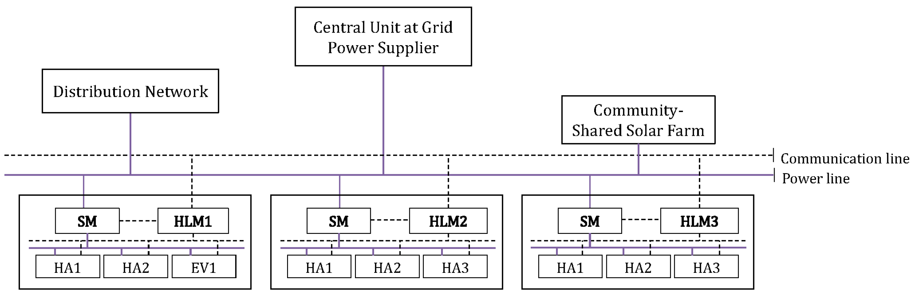
In this study, we present a new application of CSS in Korea and construct a comprehensive mathematical programming model to evaluate the performance of the proposed CSS. Our CSS comprises multiple households in a medium-sized community and a CSS business developer or operator (owned by the public or private). Both the households and CSS are assumed to be connected to the grid. The households participate in the CSS business by renting the PV panels (or capacity). The CSS supplies the electricity needed by the households using the rented capacity. The total capacity rented by the households is assumed to be only a part of the CSS business, and the main purpose of the rental service is not to make a profit but to encourage the community members to engage in economic activities with CSS [35]. The rent is on a monthly basis since Korea has four distinct seasons and this short-term rental can reduce participation risks associated with uncertain weather and load forecasts. Each household determines an optimal rental size through its own home load management (HLM) system, which smartly minimizes the electricity bill [36]. The size optimization in HLM is based on a rental price provided by the CSS operator, hourly varying demand-responded electricity prices offered by the connected grid, and a day-ahead solar radiation forecast. At the same time, each HLM also decides the loading schedule of household appliances assuming the successful rental of the desired PV capacity.

This model does not assume the presence of on-site or off-site battery storage systems for households, as it anticipates higher profitability for end-users with no or small aggregated storage units [37]. On the other hand, larger storage capacities are crucial for reducing unmanageable load variance and subsequent costs from the grid’s perspective. Similarly, for community-clustered solar-plus-battery prosumers, the most profitable scenario for all prosumers is still only the PV [38]. The CSS business has the option to install energy storage systems to maximize its own profit, but this is not accounted for in our model as it is focused on the tenant’s view. The model assumes that the CSS business will sell excess solar energy from the rented capacity to utilities and distribute the profits as a rental subsidy to the participating households. It is important to note that if the selling price is lower than the retail price from the grid to the households, a customer can make a profit by selling the surplus energy to their neighbors at a higher price [39]. In our model, customers can rent any size of PV capacity at the same price across the participants if it is profitable, and selling the surplus electricity to a participant does not occur. In Korea, the new renewable energy support scheme offers a maximum 20% increase in the renewable energy certificates multiplier when community residents are involved in the projects [40]. Additionally, the relatively low electricity retail price in Korea also supports this model.

The contribution of this study can be summarized as follows:

• This study proposes a new and simple CSS model to promote community-based participation in PV installations for land care in Korea.
• The proposed CSS application is evaluated using a mathematical programming model within a leader–follower framework. A robust solution procedure, utilizing the Karush–Kuhn–Tucker (KKT) conditions, has been developed in this study.
• The profitability of the proposed model is assessed numerically from the perspectives of three main stakeholders: the community participants, the CSS business (or the government aiming to promote CSS PV installations), and the grid power supplier [41].

The numerical results indicate that the proposed CSS model delivers substantial economic benefits across all stakeholders. Participating households experienced electricity cost reductions ranging from 36.8% to 56.7% due to decreased reliance on grid power alongside the integration of CSS. The CSS business also achieved considerable profitability through surplus electricity sales, generating up to 7007 KRW/kW in the summer season, with an overall surplus income of 6825 KRW/kW. Seasonal PV capacity rentals varied from 193 kW in spring to 1392 kW in winter, depending on the CSS project scenarios. In addition, the grid power supplier benefits from reduced fluctuations in power supply resulting from households’ participation in CSS and the subsequent demand shift.

The remainder of this paper is organized as follows: Section 2 defines the CSS PV network model that consists of the participating households with a smart meter and home-load management functions. It describes the objective functions of the CSS farm, electricity demand constraints of households, and a quadratic cost function of grid-supplied electricity. It also provides a summary of sets, parameters, and variables used in this study. Section 3 constructs a two-stage decision model for the CSS business and households with a leader–follower structure. It also provides, using KKT conditions, an iteratively interacting algorithm to solve the two-stage model. In Section 4, results of numerical evaluation are provided to explore and justify the performance of the proposed CSS PV project. The results focus on the economic benefits for all stakeholders involved, including households, the CSS business (or government), and the grid service provider. Finally, Section 5 concludes this study by summarizing the main findings and addressing its limitations.

2. System Model

We consider a smart CSS system that consists of three parties: multiple residential households (i.e., customers) with smart meters and home load managers, a CSS PV farm, and an energy service provider or a grid power supplier. As shown in Figure 1, the three parties are connected by a two-way communication link that enables them to exchange information with each other. Each customer can share a part of photovoltaic solar panels from the CSS farm by a monthly rental contract. Additionally, we assume that each customer is equipped with a smart meter that has a home load management (HLM) capability for scheduling the household energy consumption and determining the amount of an optimal PV rental capacity through communications with the CSS farm. The smart meter is connected to the power lines coming from the service provider and coming from the CSS farm. We assume that the CSS farm has enough PV capacity to sufficiently meet the rental demand from customers.

Let us define $\mathrm{N}$ as a set of households and let $\mathrm{H}$ and $\mathrm{D}$ denote a set of time slots and days considered in this study, respectively.

Table 1. Notations for sets, parameters, and variables.

Type	Symbol	Definition
Sets	$\mathcal{N}$	set of households in the power system
	${\mathcal{A}}_n$	set of household appliances at household n
	$\mathcal{H}$	set of hours during the operating horizon period
	$\mathcal{D}$	set of days during the operating horizon period
	${\mathcal{H}}_{n,a}\left(d\right)$	set of fixed operation hours of appliance a at day d
Parameters	p	CO&M cost of CSS farm
	$\alpha \left(d\right),\beta \left(d\right)$	seasonal electricity price coefficient at day d
	${\zeta }_{a_1}$	fixed energy requirement of appliance a
	$E_{n,a_2}\left(d\right)$	daily electricity requirement of appliance a at household n
	${\eta }_{n,a_2,m}$	maximum working power of appliance a at household n
	$\kappa (d,h)$	hourly power production efficiency at CSS farm site
Variables	r	rental price of CSS farm
	$y_n$	grid cost of household n
	$f_n$	total cost of household n
	$c_n$	PV capacity rented by household n
	$l_n(d,h)$	energy load profile by household n at day d and hour h
	$x_{n,a}(d,h)$	energy consumption scheduling of appliance a in household n at day d and hour h
	$g_n(d,h)$	PV energy generation profile rented by household n at day d and hour h
	$g_{n,u}(d,h)$	energy generated by PV at day d and hour h and immediately used at that time slot in household n
	$g_{n,d}(d,h)$	energy generated by PV at day d and hour h and remaining unused at that time slot in household n
	$\rho (d,h)$	hourly price profile at day d and hour h

summarizes notations for other sets, parameters, and variables used in this paper.

2.1. Rental Profit in the CSS Farm

Let r and p be a rental price and a construction plus operations and maintenance (CO&M) cost per capacity, and let $c_n$ be the capacity rented by household n. Then the total rental profit z of the CSS farm is assumed by

$$z=(r-p)\sum _n{c}_n.$$

(1)

We assume that the same rental price r is applied for every customer. If z becomes negative, the CSS business cannot be established. Thus, the CSS business should set r greater than p. However, when p is high, the range of r that is affordable to the customers certainly diminishes, and the participation of the households in the CSS business severely shrinks. Moreover, the affordability of r also depends on the price of grid-supplied electricity. We assume that the local government can subsidize the CSS PV to promote household participation, lowering the CO&M cost of rental PV.

In this study, we assume a monthly rental agreement between a customer and the CSS farm, and the profit and rents are on a monthly basis. At the start of a month, the CSS farm broadcasts to the customers a monthly forecast of efficiencies of CSS PV generation and initial rental price. The smart meter in each customer household then determines the rental capacity based on the rental price sent from the CSS farm. Collecting the PV rental demands from all the customers, the CSS farm can adjust the previous rental price to maximize its profit. If adjusted, the price is sent to the customers again, and the smart meters respond consecutively.

2.2. Electricity Generation from CSS PV for Households

Let $g_n(d,h)$ be the electricity generated from CSS PV at hour h of the dth day, which is rented by household n. We devise ($d,h$) to denote the time instance in this study and to be sometimes referred to as a time slot. $g_n(d,h)$ is determined by the product of power generation efficiency $\kappa (d,h)$ and rented PV capacity $c_n$ such that

$$g_n(d,h)=\kappa \left(h\right)c_n$$

(2)

where $\kappa \left(h\right)$ represents the PV inverter’s efficiency of DC to AC conversion, solar radiation, and temperature at the CSS farm site [42].

2.3. Power Demand from Household

Let ${\mathrm{A}}_n$ denote a set of appliances in household n. For appliance $a\in {\mathrm{A}}_n$, let $x_{n,a}(d,h)$ denote the power consumption at time ($d,h$), which is a scheduling variable handled by HLM. The total grid load $l_n(d,h)$ at time ($d,h$) from household n can then be written as

$$l_n(d,h)\ge \sum _{a\in {\mathrm{A}}_n}{x}_{n,a}(d,h)-g_{n,u}(d,h),$$

(3)

where $g_{n,u}(d,h)$ is a certain portion of PV power $g_n(d,h)$ generated at CSS PV and used for the household. Let $g_{n,d}(d,h)$ be the generated but unused PV power, then

$$g_{n,u}(d,h)+g_{n,d}(d,h)\le \kappa \left(h\right)c_n.$$

(4)

Unused PV power can be sold to an energy service provider or other communities. We assume that this surplus electricity from CSS PV is used to compensate for the subsidies paid by the local government to the CSS business.

We assume that the household appliances are categorized into inelastic- and elastic-load appliances, denoted by $a_1$ and $a_2$, respectively. An inelastic load appliance has a fixed power requirement ${\zeta }_{n,a}$ during a fixed operational interval, denoted by ${\mathrm{H}}_{n,a}\left(d\right)$. The power consumption requirement by inelastic load appliances can be defined as

$$x_{n,a_1}(d,h)=\left\{\begin{array}{cc}\ge {\zeta }_{n,a_1},\hfill & \mathrm{if}h\in {\mathrm{H}}_{n,a_1}\left(d\right),\hfill \\ 0,\hfill & \mathrm{otherwise}.\hfill \end{array}\right.$$

(5)

In contrast, an elastic load appliance can flexibly manage its power requirement between 0 and a maximum working power, ${\eta }_{n,a_2,m}$. Thus, the energy consumption by an elastic load appliance is constrained by

$$x_{n,a_2}(d,h)\le {\eta }_{n,a_2,m},\forall h\in {\mathrm{H}}_{n,a_2}\left(d\right).$$

(6)

However, it has a requirement on power consumption $E_{n,a_2}\left(d\right)$ such that

$$\sum _{h\in \mathrm{H}}{x}_{n,a_2}(d,h)\ge E_{n,a_2}\left(d\right).$$

(7)

2.4. Costs of Utilizing the Grid-Supplied Electricity

We assume a quadratic cost function for the grid electricity consumption, which is widely accepted in the smart grid literature [43]. The grid announces daily electricity price coefficients $\alpha \left(d\right)$ and $\beta \left(d\right)$ and the total load profile $L(d,h)$ through the communication network connecting all consumers. With this announced information, the hourly electricity price $\rho (d,h)$ of the grid power can be projected by

$$\rho (d,h)=\alpha \left(d\right)L(d,h)+\beta \left(d\right)=\alpha (d,h)\left({\displaystyle \sum _{n\in \mathrm{N}}}{l}_n(d,h)\right)+\beta \left(d\right).$$

(8)

Let $\overline{l}(d,h)=L(d,h)-l_n(d,h)$, then ${\overline{l}}_n(d,h)$ indicates the load requirement from the other customers except for the customer n. The hourly electricity price of the grid for household n is rewritten by

$$\rho (d,h)=\alpha \left(d\right)\left(l_n(d,h)+\overline{l}(d,h)\right)+\beta \left(d\right).$$

(9)

The household incurs monthly expenses $y_n$ for grid costs based on electricity prices and their load profile for the month such that

$$y_n=\sum _{(d,h)}\rho (d,h)l_n(d,h)=\sum _{(d,h)}\left\{\alpha \left(d\right)l_n{(d,h)}^2+\alpha \left(d\right)l_n(d,h)\left(\overline{l}(d,h)+\beta \left(d\right)\right)\right\}.$$

(10)

3. Two-Stage Decision Model for PV Rental Price and Capacity

3.1. Optimization Models for Households and the CSS Business

The determination of $c_n$ by each household n and r by the CSS business is performed by an interacting procedure between the two parties. Thus, the respective parties perform two-stage optimization. Given an initial unit rental cost r by the CSS business, each household decides an optimal rental PV capacity $c_n$ that minimizes its overall expenses $f_n$, including the rental fee and the payment to the grid electricity such that

$$f_n=\sum _{(d,h)}\rho (d,h)l_n(d,h)+r{c}_n.$$

(11)

It is noted that the first term in (11) is in a quadratic form defined by Equation (10).

Each household sends its request for rental PV capacity $c_n$ to the CSS business, and the CSS part re-calculates the rental price r with the aggregate demands from the households. The two-stage problems are defined as follows:

Stage 1: Household $\mathit{n}$’s optimization problem:

$$\begin{array}{cc}\hfill \underset{c_n,l_n(d,h),x_{n,a}(d,h),g_{n,u}(d,h)}{min}& f_n={\sum }_{(d,h)}\rho (d,h)l_n(d,h)+r{c}_n\\ \hfill \mathrm{subject}\mathrm{to}& \mathrm{c}\mathrm{o}\mathrm{n}\mathrm{s}\mathrm{t}\mathrm{r}\mathrm{a}\mathrm{i}\mathrm{n}\mathrm{t}\mathrm{s} \mathrm{i}\mathrm{n} \left(3\right)–\left(6\right), \left(9\right) \mathrm{a}\mathrm{n}\mathrm{d} \left(10\right),\\ & \left(c_n,l_n(d,h),x_{n,a}(d,h),g_{n,u}(d,h),g_{n,d}(d,h),\rho (d,h)\right)⪰0\end{array}$$

(12)

Stage 2: CSS operator’s optimization problem:

$$\begin{array}{cc}\hfill \underset{r⪰p}{max}& z=(r-p)\sum _n{c}_n.\end{array}$$

In Stage 1, the household determines $c_n$ while simultaneously deciding its load profile within the shifting capacity of the home appliances. In Stage 2, the CSS operator’s optimization problem is a constrained linear programming problem. However, since the capacity $c_n$ determined by each household is a function of r, the problem can be reformulated into a quadratic problem in r, which will be obtained by Karush–Kuhn–Tucker (KKT) analysis in the following subsections.

3.2. Relation Between PV Rental Capacity and Price

We apply KKT conditions to find an optimal $c_n$ in problem Stage 1, which is expressed by the given parameter r. KKT conditions for optimality consist of primal feasibility, dual feasibility, complementary slackness, and stationary conditions [44]. The Lagrangian function for problem Stage 1 is defined by

$$\begin{array}{ccc}\hfill L_n& =& y_n+r·c_n-{\lambda }_{n,1}(y_n-{\displaystyle \sum _{(d,h)}}\rho (d,h)l_n\left(h\right))\hfill \\ & -& {\displaystyle \sum _{(d,h)}}\left({\lambda }_{n,2}(d,h)\right(l_n(d,h)-{\displaystyle \sum _a}{x}_{n,a}(d,h)-g_{n,u}(d,h)\left)\right)\hfill \\ & -& {\displaystyle \sum _{(d,h)}}\left({\lambda }_{n,3,a_1}(d,h)(x_{n,a_1}(d,h)-{\zeta }_{n,a_1})\right)-{\displaystyle \sum _d}\left({\lambda }_{n,4,a_2}\left(d\right)\right({\displaystyle \sum _h}{x}_{n,a_2}(d,h)-E_{a_2}\left)\right)\hfill \\ & -& {\displaystyle \sum _{(d,h)}}\left({\lambda }_{n,5,a_2}(d,h)\left({\eta }_{n,a_2,m}-x_{n,a_2}(d,h)\right)\right)\hfill \\ & -& {\displaystyle \sum _{(d,h)}}\left({\lambda }_{n,6}(d,h)(\kappa (d,h)c_n-g_{n,u}(d,h)-g_{n,d}(d,h))\right)\hfill \\ & -& {\displaystyle \sum _{(d,h)}}\left({\lambda }_{n,7}(d,h)(\rho (d,h)-\alpha \left(d\right)(l_n(d,h)+\overline{l}(d,h))+\beta \left(d\right))\right)\hfill \\ & -& {\mu }_{n,1}{y}_n-{\mu }_{n,2}{c}_n-{\displaystyle \sum _{(d,h)}}\left({\mu }_{n,3}(d,h)l_n(d,h)\right)-{\displaystyle \sum _a}\left({\displaystyle \sum _{(d,h)}}\left({\mu }_{n,4,a}(d,h)x_{n,a}(d,h)\right)\right)\hfill \\ & -& {\displaystyle \sum _{(d,h)}}\left({\mu }_{n,5}(d,h)g_{n,u}(d,h)\right)-{\displaystyle \sum _{(d,h)}}\left({\mu }_{n,6}(d,h)g_{n,d}(d,h)\right)-{\displaystyle \sum _{(d,h)}}\left({\mu }_{n,7}(d,h)\rho (d,h)\right),\hfill \\ & & \lambda =\left({\lambda }_{n,1},{\lambda }_{n,2}(d,h),{\lambda }_{n,3,a_1}(d,h),{\lambda }_{n,4,a_2}\left(d\right),{\lambda }_{n,5,a_2}(d,h),{\lambda }_{n,6}(d,h),{\lambda }_{n,7}(d,h)\right),\hfill \\ & & \mu =\left({\mu }_{n,1},{\mu }_{n,2},{\mu }_{n,3}(d,h),{\mu }_{n,4,a}(d,h),{\mu }_{n,5}(d,h),{\mu }_{n,6}(d,h),{\mu }_{n,7}(d,h)\right),\hfill \end{array}$$

(13)

where $\mathit{\lambda }$ and $\mathit{\mu }$ are sets of Lagrange multipliers and dual variables of each constraint in (12). The dual feasibility ensures that the Lagrange multipliers or dual variables are non-negative. These constraints can be expressed by

$$\begin{array}{ccc}\hfill \lambda & ⪰& 0,\hfill \\ \hfill \mu & ⪰& 0.\hfill \end{array}$$

The complementary slackness conditions define the critical interaction between the constraints, the Lagrange multipliers, and the dual variables in problem Stage 1. In the optimization problem for household n, if a constraint is not binding, the corresponding Lagrange multiplier must be zero. Similarly, for the dual variables, if a dual variable is nonzero, the associated primal variables must be zero.

The stationary conditions are also a key component of KKT conditions in nonlinear optimization. It ensures that at an optimal point, the gradient of the Lagrangian function to the decision variables is equal to zero, balancing out the effects of the objective function and the constraints. The stationary conditions for problem Stage 1 are as follows:

$$\begin{array}{ccc}\hfill {\displaystyle \frac{\partial L_n}{\partial y_n}}& =& 1-{\lambda }_{n,1}-{\mu }_{n,1}=0,\hfill \end{array}$$

(14)

$$\begin{array}{ccc}\hfill {\displaystyle \frac{\partial L_n}{\partial c_n}}& =& r-{\lambda }_{n,6}(d,h)\kappa (d,h)-{\mu }_{n,2}=0,\hfill \end{array}$$

(15)

$$\begin{array}{ccc}\hfill {\displaystyle \frac{\partial L_n}{\partial l_n(d,h)}}& =& {\lambda }_{n,1}\rho (d,h)-{\lambda }_{n,2}(d,h)+{\lambda }_{n,7}(d,h)\alpha \left(d\right)-{\mu }_{n,3}(d,h)=0,\hfill \\ \hfill {\displaystyle \frac{\partial L_n}{\partial x_{n,a_1}(d,h)}}& =& {\lambda }_{n,2}(d,h)-{\lambda }_{n,3,a_1}\left(h\right)-{\mu }_{n,4,a_1}(d,h)=0,\hfill \\ \hfill {\displaystyle \frac{\partial L_n}{\partial x_{n,a_2}(d,h)}}& =& {\lambda }_{n,2}(d,h)-{\lambda }_{n,4,a_2}\left(d\right)+{\lambda }_{n,5,a_2}(d,h)-{\mu }_{n,4,a_2}(d,h)=0,\hfill \end{array}$$

(16)

$$\begin{array}{ccc}\hfill {\displaystyle \frac{\partial L_n}{\partial g_{n,u}(d,h)}}& =& -{\lambda }_{n,2}(d,h)+{\lambda }_{n,6}(d,h)-{\mu }_{n,5}(d,h)=0,\hfill \\ \hfill {\displaystyle \frac{\partial L_n}{\partial g_{n,d}(d,h)}}& =& {\lambda }_{n,6}(d,h)-{\mu }_{n,6}(d,h)=0,\hfill \end{array}$$

(17)

$$\begin{array}{ccc}\hfill {\displaystyle \frac{\partial L_n}{\partial {\rho }_n(d,h)}}& =& {\lambda }_{n,1}{l}_n(d,h)-{\lambda }_{n,7}(d,h)-{\mu }_{n,7}(d,h)=0.\hfill \end{array}$$

(18)

By solving Equations (14) and (16)–(18), ${\lambda }_{n,6}(d,h)$ can be obtained as follows:

$$\begin{array}{ccc}\hfill {\lambda }_{n,6}(d,h)& =& \rho (d,h)+\alpha \left(d\right)\left(l_n(d,h)-{\mu }_{n,7}(d,h)\right)-{\mu }_{n,3}(d,h)\hfill \\ & =& \alpha \left(d\right)\left(2\left(\sum _a{x}_{n,a}(d,h)-\kappa (d,h)c_n+g_{n,d}(d,h)\right)+\overline{l}(d,h)-{\mu }_{n,7}(d,h)\right)\hfill \end{array}$$

(19)

$$\begin{array}{ccc}& & +\beta \left(d\right)-{\mu }_{n,3}(d,h)+{\mu }_{n,5}(d,h).\hfill \end{array}$$

(20)

By substituting $l_n(d,h)$ from Equations (3) and (4) into Equation (19), the expression can be reformulated as a capacity-based equation, as shown in Equation (20). By substituting Equation (20) into Equation (15), the equation explaining the relationship between r and $c_n$ is established by

$$c_n={\displaystyle \frac{B_n(d,h)-r}{D(d,h)}},$$

(21)

where

$$D(d,h)=\sum _{(d,h)}2\alpha \left(d\right)\kappa {(d,h)}^2,$$

(22)

and

$$\begin{array}{c}\hfill B_n(d,h)=\sum _{(d,h)}\left(\alpha \left(d\right)\left(2\left(\sum _a{x}_{n,a}(d,h)+g_{n,d}(d,h)\right)+\overline{l}(d,h)-{\mu }_{n,7}(d,h)\right)+\beta \left(d\right)-{\mu }_{n,3}(d,h)+{\mu }_{n,5}(d,h)\right)\kappa (d,h)+{\mu }_{n,2},\end{array}$$

(23)

3.3. Modified Stage 2 Problem and Finding an Optimal Rental Price for the CSS Business

By substituting Equation (21) into the objective function of problem Stage 2 for the CSS business, we can have

$$z=(r-p){\displaystyle \frac{{\sum }_n\left(B_n(d,h)-r\right)}{D(d,h)}},$$

(24)

which is a quadratic function according to r. Thus, problem Stage 2 can be modified as follows:

Modified Stage 2: CSS operator’s optimization problem:

$$\begin{array}{cc}\hfill \underset{r⪰p}{max}& z=(r-p){\displaystyle \frac{{\sum }_n\left(B_n(d,h)-r\right)}{D(d,h)}},\end{array}$$

(25)

$$\begin{array}{cc}\hfill \mathrm{subject}\mathrm{to}& \mathrm{c}\mathrm{o}\mathrm{n}\mathrm{s}\mathrm{t}\mathrm{r}\mathrm{a}\mathrm{i}\mathrm{n}\mathrm{t}\mathrm{s} \mathrm{i}\mathrm{n} \left(22\right) \mathrm{a}\mathrm{n}\mathrm{d} \left(24\right).\end{array}$$

(26)

By differentiating Equation (25) with respect to r, an optimal $r^{*}$ that maximizes z can be easily obtained as follows:

$$\begin{array}{ccc}\hfill {\displaystyle \frac{dz}{dr}}& =& {\displaystyle \frac{{\sum }_n\left(B_n(d,h)\right)-2n\left(\mathrm{N}\right)r+n\left(\mathrm{N}\right)p}{D(d,h)}}=0,\hfill \end{array}$$

(27)

$$\begin{array}{ccc}\hfill r^{*}& =& {\displaystyle \frac{{\sum }_n\left(B_n(d,h)\right)+n\left(\mathrm{N}\right)p}{2n\left(\mathrm{N}\right)}}.\hfill \end{array}$$

(28)

Table 2. Two-stage interacting iterative algorithm.

Step 0.	Set $\mathit{i}=0$, an initial reference solution
	${\theta }_n^{\left(i\right)}=\left(l_n^{\left(i\right)},c_n^{\left(i\right)}\right)=(\mathbf{0},0)$, and an initial rental price $r^{\left(i\right)}$.
	Calculate $D(d,h)$. Set $ϵ>0$.
Step 1	For $n\in \mathrm{N}$, each household solves Stage 1 and finds ${\theta }_n^{\left(i\right)}$.
	For $n\in \mathrm{N}$, calculate $B_n(d,h)$ and report $c_n$, $l_n(d,h)$ and $B_n(d,h)$ to the CSS business.
Step 2	CSS operator solves Modified Stage 2 and finds an optimal r.
Step 3	If $i\ne 0$, $\left(r^{\left(i\right)}/r^{(i-1)}-1\right)\le ϵ$ and $ma{x}_n\left({\theta }_n^{\left(i\right)}/{\theta }_n^{(i-1)}-1\right)\le ϵ$, then terminate.
	Otherwise, $i=i+1$ and update $r^{\left(i\right)}$. Furthermore, go to Step 1.

summarizes the interacting two-stage procedure for the households and the CSS business. Step 0 initializes the loads and rental capacities and computes $D(d,h)$ defined in (22). Step 1 solves the household n’s optimization problem and iterates over all households with rental price $r^{\left(i\right)}$. With an optimal solution, the value of $B_n(d,h)$ is computed as a part of the solution, and the results for $c_n,l_n(d,h)$, and $B_n(d,h)$ are reported to the CSS business. In Step 2, the optimization problem of modified Stage 2 for the CSS operator is solved using those values reported by the households. In Step 3, termination conditions to stop the procedure are tested. Unless the conditions are met, the procedure proceeds in Step 1 with updated $r^{\left(i\right)}$ and load profiles.

4. Numerical Results

4.1. Simulation Setup

We evaluated the performance of the proposed CSS model and interacting two-stage procedure with four nonconsecutive months. Each month represents a typical weather and electricity demand pattern for the respective seasons: spring, summer, autumn, and winter. The results from those months are compared to identify a seasonal effect of the CSS implementation. The evaluation model simulates 400 households participating in the CSS project, consisting of three types of households: single-person (1P), two-person (2P), and three-or-more-person (3P) households. We designed the daily electricity demand that varies according to these household types. 3P households consume the most electricity, followed by 2P and 1P households. The proportion of the three household types was determined based on a survey report for Korean household appliances [19], with 1P accounting for 36.8%, 2P for 29.8%, and 3P for 33.5% of the all 400 households.

The electricity demand from appliances installed in each household is depicted in

Table 3. Appliance power consumption and usage time.

Season	Class	Type	Power Consumption (kW)	Average Daily Usage Time (h)
All seasons	Inelastic	General refrigerator	0.0422	24
		Kimchi refrigerator	0.0193	24
	Elastic	TV	0.1515	6
		Clothes dryer	1.3628	1
		Washing machine	0.9914	1
		Electric stove	2.6908	2
		Electric rice cooker	1.0500	1
		Hair dryer	1.5061	1
		Air purifier	0.0491	12
		Mobile	0.0165	5
		Standard EV charger	3.5	1
Summer	Elastic	Dehumidifier	0.2707	5
		Fan	0.0437	7
		Air conditioner	1.5980	5
Winter	Elastic	Electric heated bed	0.4116	8
		Electric blanket	0.1708	7
		Water heated pad	0.3323	8
		Humidifier	0.0375	6
		Electric heater	1.0294	4

. The values are derived from [45] based on power consumption, usage hours, and energy usage data. The specification for electric vehicle (EV) charging is sourced from [46]. Specifically, standard chargers consume 7 kW, and a single charge takes approximately 5 h. However, since EVs are not charged daily, the power consumption is assumed to be 3.5 kW, which is 50% of the full load, and the average daily charging time is assumed to be 1 h. Appliance usage times specified in the table are adjusted randomly for each household to account for different usage times. Random adjustments are applied according to household type: for 1P households, random values follow a uniform (−1, 2) distribution; for 2P households, uniform (0, 1); and for 3P households, uniform (0, 2). These random values are added to the average daily usage time to determine each household’s daily usage. The daily electricity consumption is calculated using adjusted usage times and power consumption. Fixed consumption patterns were created for each household and appliance based on the daily electricity consumption. For instance, a household may have a pattern of watching TV for 3 h at 6, 7, and 8 PM. These patterns were established for each household and appliance, considering cultural factors specific to Korea, such as the common practice of avoiding noisy appliances like vacuum cleaners or washing machines during late-night hours in shared residential buildings such as apartments to prevent disturbing neighbors.

Table 4. Average monthly electricity consumption by household types and seasons (unit: kW).

Household Type	Spring	Summer	Autumn	Winter
1P	233	500	241	465
2P	434	766	449	796
3P	591	966	611	1001

shows the average monthly electricity consumption by household type and season, illustrating how the established consumption patterns result in seasonal electricity demand for different household types.

The coefficients of the electricity cost function in (8) are approximately derived by using the Korean progressive electricity tariff system specified in [47] and summarized in

Table 5. Seasonal coefficients of the electricity cost function (unit: KRW/kW, KRW).

Season	$\mathit{\alpha }\mathbf{\left(}\mathit{d}\mathbf{\right)}$	$\mathit{\beta }\mathbf{\left(}\mathit{d}\mathbf{\right)}$
Spring/Autumn	0.931	0.337
Summer	0.994	0.337
Winter	1.051	0.337

. The price per unit of electricity consumption in winter is relatively higher than that for other seasons, which results from the higher electricity demand for heating in winter in Korea.

We assumed that CO&M cost p per PV capacity is a certain percentage of the sum of the CapEx (Capital Expenditure) and the annual fixed O&M cost of the PV farm. These CapEx and O&M costs were referenced from [48], and the 2023 annual average exchange rate (USD 1 = 1288 KRW) was applied. We assumed that a local government subsidizes a part of the actual CO&M cost. This subsidy aims to finally reduce households’ CSS PV rental costs, diminishing the financial burden and encouraging CSS PV adoption. In the simulation, we assumed that the subsidy covers 10% of the total CO&M cost. The percentage is used as a baseline and projected from the Korean electricity price structure [47] and the PV CO&M cost in [48,49]. This high-cost level implies that the electricity price in Korea is still too low to facilitate the PV installation. In Section 4.5, the subsidy percentage changes for sensitivity analysis.

To determine the power generation efficiency of CSS PV, we have used the climate data from Sunchang, Jeollabuk-do, the region with the largest solar farm area in Korea, in 2023. The data include solar radiation ($I(d,h)$) and ambient temperature ($t_0(d,h)$) [50]. Specifically, module temperature ($t_m(d,h)$) was estimated based on [51]. The efficiency ($\eta =0.2041$) and temperature coefficient of the maximum power (${\delta }_p=0.0042$) of the PV panels were obtained from the data sheet in [52]. The same data sheet was used to calculate the panel area (S = 2.6 m²/kW), which was then converted to panel area per unit capacity ($c_n$). $loss$ is also considered as the sum of the conversion loss from DC to AC (0.0188) [53] and the distribution loss (0.0199) [54] from the CSS farm to households. The power generation efficiency of CSS PV is finally determined by the following Equation [42]:

$$\kappa (d,h)=\eta SI(d,h)\left(1-{\delta }_p\left(t_m(d,h)-25\right)\right)·(1-loss).$$

(29)

To evaluate the effectiveness of CSS PV by rent in reducing grid dependency and overall electricity costs, we devise and compare two primary scenarios: CSS PV with and without demand-shift functions in households. Those scenarios are referred to as PVDS and PVND in this study, respectively. In PVND, CSS PV power supplements the fixed consumption pattern in a household, replacing part of the grid electricity. In the PVDS, a demand-shift strategy is combined with PVND to optimize electricity consumption patterns further, concentrating electricity use during abundant PV generation periods and minimizing grid reliance. In addition, for the purpose of comparison, we devise a base scenario where households rely solely on the grid power with no demand shift adjustments, which is briefly referred to as a base. In each simulation, we consider a monthly operating horizon divided into 744 (24 h × 31 days) equal time slots, denoted by $\mathrm{H}=\{1,2,3,\cdots ,24\}$ and $\mathrm{D}=\{1,2,3,\cdots ,31\}$.

4.2. Comparison of Electricity Consumption and Customers’ Benefits

This subsection presents the numerical results for the scenarios that assess the impact of CSS PV on power consumption and the participants’ benefits in cost reduction.

Figure 2a,b present the results from the base scenario. The first figure shows the average grid electricity consumption per hour by season for all households, while the second figure illustrates the corresponding grid electricity prices. Since the price is dependent on the amount of electricity consumed, the patterns in the consumption and price graphs are remarkably similar. The differences in seasonal power demand from appliances and cost function coefficients between spring and autumn are very small, resulting in negligible variations in electricity consumption and, hence, the price between these two seasons.

Figure 3 and Figure 4 present the electricity supply and consumption for the scenarios PVND and PVDS, respectively. The figures demonstrate the grid electricity supply (by blue bars), CSS PV generation (red plus green bars), CSS PV power used by households (red bars), CSS PV power unused by households (green bars, referred to as surplus electricity in this study), and the total power consumed by households.

In the PVND scenario, households maintain a fixed consumption pattern while integrating CSS PV power to partially replace the grid electricity. As a result, grid electricity usage decreases during PV generation periods. Moreover, CSS PV leads to surplus electricity, especially during the daytime when solar irradiance is at its peak. In Figure 3b, for summer, the contribution of CSS PV generation is particularly prominent, resulting in a reduced dependency on the grid. Figure 5 describing PV generation efficiency allows for an understanding of the seasonal differences in generation. In spring, the highest efficiency is achieved, but due to relatively low electricity demand, the contribution of CSS PV generation is less significant compared to summer. In summer, abundant solar irradiance results in higher PV generation, and the greater electricity demand further emphasizes the role of CSS PV power. In autumn, stable PV efficiency is maintained, contributing consistently to reducing grid electricity usage. In contrast, winter shows the lowest generation and efficiency, leading to the smallest contribution from CSS PV power. As a result, PV power rented from the CSS farm contributes to reducing electricity costs across all seasons. In particular, summer achieves the most substantial cost savings due to the highest solar irradiance. Spring and autumn, with their stable PV generation, show similar cost reduction effects, while winter, despite low solar irradiance, still manages to contribute to some cost savings.

In the PVDS scenario, the combination of CSS PV and demand- shift functions in households aims to minimize dependency on the grid and maximize electricity cost savings. This scenario optimizes consumption patterns by concentrating electricity use during CSS PV generation periods. As seen in Figure 4, the PVDS scenario achieved higher efficiency in PV power usage than the PVND scenario. This resulted in minimizing surplus electricity by demand shifts and a more effective replacement of grid power with CSS PV power. In the PVDS scenario, CSS PV power contributed 18.9–37.9% of total electricity consumption, while the grid electricity accounted for 49.2–73.2%, indicating that CSS PV power was more effectively replacing grid electricity. This increased utilization of CSS PV power, particularly during daylight hours, substantially reduced grid electricity consumption and, hence, payments. Due to demand shifts, the grid electricity usage remained stable during PV generation periods, and peak electricity demand significantly declined. Consequently, the cost-effectiveness of CSS PV adoption improved considerably in the PVDS scenario.

Table 6. Monthly average payments for household electricity consumption and their shares between electricity sources, grid, and PV rent for PVND and PVDS scenarios across four seasons.

Scenario	Season	Payment (Thousand KRW)			Share of Cost (%)
		Total	Grid	Rent	Grid	Rent
Base	Spring	94.95	94.95	-	100.0	-
	Summer	296.51	296.51	-	100.0	-
	Autumn	98.11	98.11	-	100.0	-
	Winter	320.63	320.63	-	100.0	-
PVND	Spring	80.75 (−15.0%)	74.15 (−21.9%)	6.59	91.8	8.2
	Summer	228.33 (−23.0%)	204.61 (−31.0%)	23.72	89.6	10.4
	Autumn	80.26 (−18.2%)	72.50 (−26.1%)	5.27	90.3	9.7
	Winter	295.11 (−8.0%)	283.12 (−11.7%)	11.98	95.9	4.1
PVDS	Spring	59.75 (−37.1%)	46.15 (−51.4%)	13.82	77.0	23.0
	Summer	128.24 (−56.8%)	78.24 (−73.6%)	48.12	62.1	37.9
	Autumn	55.58 (−43.4%)	39.22 (−60.0%)	16.37	71.4	28.6
	Winter	200.93 (−37.3%)	162.85 (−49.2%)	38.07	81.0	18.9

and

Table 7. Monthly average electricity consumption for households and their shares between electricity sources, grid, and PV, for PVND and PVDS scenarios across four seasons.

Scenario	Season	Electricity Source (kWh)			Share of Electricity (%)
		Total	Grid	PV	Grid	PV
Base	Spring	412.8	412.8	-	100.0	-
	Summer	735.0	735.0	-	100.0	-
	Autumn	426.6	426.6	-	100.0	-
	Winter	743.1	743.1	-	100.0	-
PVND	Spring	412.8	366.4	46.4	88.7	11.3
	Summer	735.0	599.9	135.1	81.6	18.4
	Autumn	426.6	368.5	58.6	86.4	13.6
	Winter	743.1	683.5	59.5	92.0	8.0
PVDS	Spring	412.8	293.2	119.6	71.0	29.0
	Summer	735.0	379.3	355.6	51.6	48.4
	Autumn	426.6	276.8	147.7	64.9	35.1
	Winter	743.1	527.0	216.1	70.9	29.1

summarize and compare the monthly total payments per household and the shares of electricity sources between CSS PV and the grid by the household for base, PVND, and PVDS scenarios. The percentages in parentheses in Table 6 represent the differences between the base and each of the other scenarios. The total payment reduction between the base and PVND scenarios ranges from approximately 8.0% in winter to 23.0% in summer, while the reduction between the base and PVDS scenarios varies from about 37.3% in winter to 56.7% in summer. The highest payment reduction in each of the PVND and PVDS scenarios accompanies the highest share of CSS PV electricity in the total power consumption: 18.4% in PVND and 48.4% in PVDS. The PVDS scenario minimizes reliance on the grid and achieves significant cost savings across all seasons, by which the household’s benefits are maximized.

4.3. Grid Service Provider’s Benefits

Although grid electricity usage and payments to the grid decrease, this reduction rather plays a positive role by reducing fluctuations in the power supply and enhancing stability, ultimately lowering operational costs and increasing profitability for the grid. Moreover, it contributes to speeding up the so-called greenization of electricity supply.

Table 8. Seasonal averages and standard deviations of electricity supply from grid for different scenarios (unit: kWh).

Scenario	Spring		Summer		Autumn		Winter
	Average	std	Average	std	Average	std	Average	std
Base	229.33	63.12	395.14	64.20	229.33	63.12	399.50	65.41
PVND	203.53	52.48	322.53	80.93	198.09	50.54	367.50	98.23
PVDS	162.89	31.00	203.94	37.62	148.82	26.75	283.31	54.51

shows the seasonal averages and standard deviations of grid electricity supply under each scenario. In the base scenario, where no PV generation is assumed, the grid dependency is high across all seasons, resulting in high variability in grid power usage, especially in summer and winter. In the PVND scenario, CSS PV generation is utilized during daylight hours, reducing overall grid usage and lowering its standard deviation. However, variability persists due to differences in power usage between PV generation and nongeneration periods, as seasonal patterns concentrate power usage during the daytime in summer and at night in winter. Additionally, the high PV capacity demand (see

Table 9. Composition of CSS incomes: rents, CO&M costs, subsidies, surplus-electricity income for PVND and PVDS scenarios across four seasons. The rented PV capacities to households are also displayed.

Scenario	Season	Total (KRW/kW)	Rent (KRW/kW)	CO&M (kRW/kW)	Subsidy (KRW/kW)	Surplus Income (KRW/kW)	Rental Capacity (kW)
PVND	Spring	65	13,676	15,123	1512	5794	193
	Summer	182	13,793			6825	686
	Autumn	80	13,691			4768	227
	Winter	70	13,681			1418	350
PVDS	Spring	136	13,748	15,123	1512	1418	402
	Summer	370	13,982			2095	1392
	Autumn	163	13,774			1675	462
	Winter	221	13,833			1895	1101

) in both summer and winter further contributes to a higher standard deviation. In the PVDS scenario, a demand-shift strategy aligns electricity consumption more closely with PV generation periods. This adjustment significantly reduces the standard deviation of grid electricity usage across all seasons, producing the most stable supply pattern. By shifting demand to PV generation times, seasonal power usage patterns are better aligned with PV output, reducing overall grid reliance and fluctuations in grid supply. The decrease in standard deviation (std) thus reflects reduced variability, enhancing operational stability and contributing to potential cost savings and profitability for the grid service provider.

4.4. CSS PV Operator’s Economy

The implementation of CSS PV should generate economic benefits not only for households but also for the CSS business, which will contribute to enlarging green electricity production toward a net-zero economy. Through PV rentals, the CSS business has income from rent and probably a certain subsidy from a local or central government that would encourage the CSS electricity supply. In addition, it can profit by income from surplus electricity, especially during high-irradiance daytime after meeting the demand from households. Table 9 summarizes the monthly income statement of the CSS business, including rents, CO&M cost, subsidy, and surplus income per kilowatt of rented capacity. The surplus income is not included in the total. The rental rates are almost the same for seasons and scenarios. The total income with PVDS is greater than that with PVND, which results from the generally high PV capacity leased by the households. However, accounting for the surplus, the CSS business gains more income with PVND than with PVDS due to the inability of households to flexibly adjust their electricity demands to the high PV generation time. For both PVND and PVDS scenarios, the total and surplus incomes are maximized in summer with the greatest PV capacity rented, in which the household benefits were also maximized, as seen in Table 6. Notably, in the PVDS scenario, 1392 kW of PV capacity was rented during the summer, leading to a substantial increase in the operator’s rental income to 370 KRW/kW. Winter following summer was also a good season for the CSS business to generate a sufficient income statement.

The main focus should be the subsidy level that covers part of the costs of the CSS business, as it leverages the sustainability of the CSS PV for rent. With the 10% subsidy level in the simulation, the surplus income is greater than the subsidy in most cases tested except for the following two cases: the winter case with PVND and the spring case with PVDS. However, accounting for the four months, the CSS PV rent is profitable even without the subsidy. However, since the goal of CSS PV with rent includes the enlargement of PV installations and usage toward green electricity generation, a certain level of subsidy would be necessary. In the following section, the effect of subsidy levels on the PV share on electricity consumption and the profitability of the CSS business is investigated.

4.5. Sensitivity: Subsidy Ratios

To investigate how sensitive the CSS business income and customer benefits are to changes in the subsidy level, further simulation was performed with subsidy variations ranging from 0% to 50%.

Table 10. The effect of subsidy ratios on CSS incomes: rents, CO&M costs, subsidies, surplus-electricity income for PVND and PVDS scenarios. The rented PV capacities to households are also displayed. Values are averages of four seasons.

Subsidy Ratio (%)	Total (KRW/kW)	Rent (KRW/kW)	CO&M (kRW/kW)	Subsidy (KRW/kW)	Surplus Income (KRW/kW)	Rental Capacity (kW)
0%	206	15,329	15,123	-	1612	784
10%	223	13,834		1512	1772	839
20%	239	12,338		3025	1925	901
30%	258	10,844		4537	2061	971
40%	280	9354		6049	2158	1052
50%	305	7866		7562	2181	1142

presents the monthly average income changes of the CSS business according to the subsidy ratios. Without the subsidy, the CSS business generates a positive gross income (as a sum of the total plus surplus incomes) of 1818 KRW/kW. With the increasing subsidy ratio, the rental price accordingly decreases and, as a result, the PV capacity rented, the surplus income from the surplus PV generation, and finally, the total income increase. The income generated from surplus electricity can only cover 10% of the subsidy levels in the simulation. For subsidy levels between 20% and 50%, the surplus income could cover approximately 64% to 29% of the subsidies. While these economic losses from the CSS business may seem significant, they are sometimes justified by the increased share of green PV electricity in overall power consumption, which could be a key objective of the community’s CSS initiative. Furthermore, great participation from households boosts the likelihood of successfully launching PV utilities, making the losses affordable.

Table 11. The effect of subsidy ratios on household payments and their shares between bills from the grid and PV rents and shares between electricity sources. Values are averages of four seasons.

Subsidy Ratio (%)	Total Payment Difference (%)	Share of Cost (%)		Share of Electricity (%)
		Grid	Rent	Grid	PV
0%	−40.79	73.64	26.36	66.76	33.24
10%	−43.63	72.47	27.26	64.61	35.27
20%	−46.44	72.21	27.79	62.39	37.61
30%	−49.47	71.68	28.33	60.04	39.96
40%	−52.65	71.36	28.64	57.59	42.41
50%	−55.90	71.59	28.41	55.20	44.80

provides the monthly average changes of the payments and the shares of electricity consumption in the households according to the subsidy ratios. Without the subsidy, the households enjoy a 40.8% reduction in their electricity bills by taking part in the CSS project with a PV share of 33.2%. With the increasing subsidy ratio, the leased PV capacity increases as in Table 10 with the decreasing rental price per unit capacity, leading to enlarging the PV share in electricity consumption. For the subsidy levels from 10% to 50%, the PV share increases from 35.3% to 44.8%, from which the households experience up to 55.9% reduction in their payments. The sensitivity analysis demonstrates that increasing subsidies substantially improves the CSS and household profitability, contributing to a greater chance in successful PV installations and an increased share of PV generation as an energy source.

5. Conclusions

This study examined the benefits for stakeholders participating in the CSS PV project that utilizes a rental service. Various forms of CSS have also been explored in countries worldwide, demonstrating effectiveness in reducing energy costs and efficiently supplying renewable energy. The implementation of different forms of CSS can be tailored to local economic and environmental conditions as well as technological combinations. In this study, the proposed CSS model featuring PV rentals and demand-shift capabilities in households is viewed as a promising solution that encourages the adoption of solar energy while alleviating some financial burdens associated with the PV business. Furthermore, it may help to reduce local resistance to solar PV installations and accelerate the transition towards greener electricity generation.

In particular, the PVDS scenario, incorporating a demand shift strategy, optimized consumption patterns during PV generation periods by effectively managing surplus electricity and significantly reducing grid usage. These results provide economic benefits for both households and the CSS PV business. At the same time, the observed reductions in grid power costs across various scenarios reflect decreased grid dependency and enhance supply stability by lowering variability in grid electricity usage. This reduced variability contributes to operational cost savings and power-plant redundancy reduction, increasing profitability for grid operators. The sensitivity analysis of subsidy ratios revealed that higher subsidies have a substantial impact on household adoption of PV capacity. As seen in Table 11, in the PVDS scenario with a 50% subsidy, households were able to adopt PV capacity greatly, saving 56% on payments, leading to a substantial decrease in grid electricity usage and reaching a 45% share of PV electricity.

However, this study also has some limitations. The DS-based model in this study does not fully describe the behavior of demand-shifting appliances, which does not accurately account for the potential time-of-use cost savings from demand shifts. A more refined model that incorporates detailed user behavior patterns and appliance-specific constraints could offer a more precise analysis of the effects of demand shifts. Additionally, the current model does not account for battery-related technologies, while demand is concentrated during periods of PV generation and evenly distributed at other times with the demand-shift functions; this includes home batteries or vehicle-to-grid technologies that could provide additional, comparable cost savings during hours when solar energy is not available. These aspects are left for future research.

References

1. IRENA. Renewable Capacity Statistics 2023; International Renewable Energy Agency: Abu Dhabi, United Arab Emirates, 2023. [Google Scholar]
2. IEA. Electricity Market Report 2023; International Energy Agency: Paris, France, 2023. [Google Scholar]
3. IEA. Renewables 2023; International Energy Agency: Paris, France, 2024. [Google Scholar]
4. IEA. Net Zero by 2050; International Energy Agency: Paris, France, 2021. [Google Scholar]
5. KEA. 2022 New and Renewable Energy Supply Statistics; Korea Energy Agency: Ulsan, Republic of Korea, 2023. [Google Scholar]
6. MOTIE. 8th Basic Plan for Long-term Electricity Supply and Demand; Ministry of Trade, Industry and Energy: Sejong-si, Republic of Korea, 2017. [Google Scholar]
7. MOTIE. 10th Basic Plan for Long-Term Electricity Supply and Demand; Ministry of Trade, Industry and Energy: Sejong-si, Republic of Korea, 2023. [Google Scholar]
8. Choo, H.; Kim, Y.G.; Kim, D. Power sector carbon reduction review for South Korea in 2030. Renew. Sustain. Energy Rev. 2024, 196, 114348. [Google Scholar] [CrossRef]
9. SolarPower Europe. Global Market Outlook for Solar Power 2023–2027; SolarPower Europe: Brussels, Belgium, 2023. [Google Scholar]
10. IEA. Renewables 2022; International Energy Agency: Paris, France, 2022. [Google Scholar]
11. Mackenzie, W. Commodity Market Report Global solar PV Market Outlook Update: Q3 2023; Wood Mackenzie: Edinburgh, UK, 2023. [Google Scholar]
12. NEA. Renewable Energy Statistics; National Energy Administration of China: Beijing, China, 2023. [Google Scholar]
13. Commission, E. Renewable Energy Statistics; European Commission: Brussels, Belgium, 2023. [Google Scholar]
14. SEIA. Solar Market Insight Report Q2 2023; Solar Energy Industries Association: Washington, DC, USA, 2023. [Google Scholar]
15. Tanujaya, R.R.; Lee, C.Y.; Woo, J.; Huh, S.Y.; Lee, M.K. Quantifying public preferences for community-based renewable energy projects in South Korea. Energies 2020, 13, 2384. [Google Scholar] [CrossRef]
16. Bae, J.H.; Rishi, M.; Li, D. Consumer preferences for a green certificate program in South Korea. Energy 2021, 230, 120726. [Google Scholar] [CrossRef]
17. Nilson, R.S.; Stedman, R.C. Are big and small solar separate things?: The importance of scale in public support for solar energy development in upstate New York. Energy Res. Soc. Sci. 2022, 86, 102449. [Google Scholar] [CrossRef]
18. Widmer, J.; Christ, B.; Grenz, J.; Norgrove, L. Agrivoltaics, a promising new tool for electricity and food production: A systematic review. Renew. Sustain. Energy Rev. 2024, 192, 114277. [Google Scholar] [CrossRef]
19. Statistics Korea. Report on the Population and Housing Census; Statistics Korea: Daejeon, Republic of Korea, 2021.
20. Feldman, D.; Brockway, A.M.; Ulrich, E.; Margolis, R. Shared Solar. Current Landscape, Market Potential, and the Impact of Federal Securities Regulation; National Renewable Energy Laboratory (NREL): Golden, CO, USA, 2015. [Google Scholar]
21. Narjabadifam, N.; Fouladvand, J.; Gül, M. Critical review on community-shared solar—Advantages, challenges, and future directions. Energies 2023, 16, 3412. [Google Scholar] [CrossRef]
22. OSTI. Community Shared Solar: Policy and Regulatory Considerations. Available online: https://www.osti.gov/biblio/1158420 (accessed on 10 November 2024).
23. SEIA. Community Solar; Solar Energy Industries Association: Washington, DC, USA, 2023. [Google Scholar]
24. U.S. Department of Energy. Community Solar; U.S. Department of Energy: Washington, DC, USA, 2021.
25. REScoop. Community Energy; REScoop: Brussels, Belgium, 2023. [Google Scholar]
26. Caballero, V.; Briones, A.; Coca-Ortegón, A.; Pérez, A.; Barrios, B.; de la Mano, M. Analysis and simulation of an Urban-Industrial Sustainable Energy Community: A use case in San Juan de Mozarrifar using photovoltaic energy. Energy Rep. 2023, 9, 1589–1605. [Google Scholar] [CrossRef]
27. Ascione, F.; Bianco, N.; Mauro, G.M.; Napolitano, D.F.; Vanoli, G.P. Comprehensive analysis to drive the energy retrofit of a neighborhood by optimizing the solar energy exploitation—An Italian case study. J. Clean. Prod. 2021, 314, 127998. [Google Scholar] [CrossRef]
28. Syed, M.M.; Hansen, P.; Morrison, G.M. Performance of a shared solar and battery storage system in an Australian apartment building. Energy Build. 2020, 225, 110321. [Google Scholar] [CrossRef]
29. Diahovchenko, I.; Petrichenko, L. Comparative Analysis of Power Distribution Systems with Individual Prosumers Owing Photovoltaic Installations and Solar Energy Communities in Terms of Profitability and Hosting Capacity. Energies 2022, 15, 8837. [Google Scholar] [CrossRef]
30. Canova, A.; Lazzeroni, P.; Lorenti, G.; Moraglio, F.; Porcelli, A.; Repetto, M. Decarbonizing residential energy consumption under the Italian collective self-consumption regulation. Sustain. Cities Soc. 2022, 87, 104196. [Google Scholar] [CrossRef]
31. Mustafa, J.; Almehmadi, F.A.; Alqaed, S.; Sharifpur, M. Building a sustainable energy community: Design and integrate variable renewable energy systems for rural communities. Sustainability 2022, 14, 13792. [Google Scholar] [CrossRef]
32. Karunathilake, H.; Hewage, K.; Prabatha, T.; Ruparathna, R.; Sadiq, R. Project deployment strategies for community renewable energy: A dynamic multi-period planning approach. Renew. Energy 2020, 152, 237–258. [Google Scholar] [CrossRef]
33. IEA. Renewables 2021; International Energy Agency: Paris, France, 2021. [Google Scholar]
34. WRI. Why Community Solar Should Be Part of the Equation; World Resources Institute: Washington, DC, USA, 2019. [Google Scholar]
35. ESMAP. Market Outlook and Handbook for Decision Makers; Energy Sector Management Assistance Program: Washington, DC, USA, 2023. [Google Scholar]
36. Jung, S.; Kim, D. Pareto-efficient capacity planning for residential photovoltaic generation and energy storage with demand-side load management. Energies 2017, 10, 426. [Google Scholar] [CrossRef]
37. Freitas, S.; Reinhart, C.; Brito, M. Minimizing storage needs for large scale photovoltaics in the urban environment. Solar Energy 2018, 159, 375–389. [Google Scholar] [CrossRef]
38. Aranzabal, I.; Gomez-Cornejo, J.; López, I.; Zubiria, A.; Mazón, J.; Feijoo-Arostegui, A.; Gaztañaga, H. Optimal management of an energy community with PV and battery-energy-storage systems. Energies 2023, 16, 789. [Google Scholar] [CrossRef]
39. Lee, S.; Shenoy, P.; Ramamritham, K.; Irwin, D. AutoShare: Virtual community solar and storage for energy sharing. Energy Inform. 2021, 4, 10. [Google Scholar] [CrossRef]
40. KEA. National Survey Report of PV Power Applications in Korea; Korea Energy Agency: Ulsan, Republic of Korea, 2022. [Google Scholar]
41. Chaurey, A.; Kandpal, T.C. A techno-economic comparison of rural electrification based on solar home systems and PV microgrids. Energy Policy 2010, 38, 3118–3129. [Google Scholar] [CrossRef]
42. Wan, C.; Zhao, J.; Song, Y.; Xu, Z.; Lin, J.; Hu, Z. Photovoltaic and solar power forecasting for smart grid energy management. CSEE J. Power Energy Syst. 2015, 1, 38–46. [Google Scholar] [CrossRef]
43. Mohsenian-Rad, A.H.; Wong, V.W.; Jatskevich, J.; Schober, R.; Leon-Garcia, A. Autonomous demand-side management based on game-theoretic energy consumption scheduling for the future smart grid. IEEE Trans. Smart Grid 2010, 1, 320–331. [Google Scholar] [CrossRef]
44. Boyd, S.; Vandenberghe, L. Convex Optimization; Cambridge University Press: Cambridge, UK, 2004. [Google Scholar]
45. KPX. 2019 Survey on Household Appliance Deployment; Korea Power Exchange: Naju, Republic of Korea, 2020. [Google Scholar]
46. KPX. Analysis of the Deployment and Utilization of Electric Vehicles and Chargers; Korea Power Exchange: Naju, Republic of Korea, 2023. [Google Scholar]
47. KEPCO. Electricity Tariff Structure. Available online: https://online.kepco.co.kr/PRM015D00 (accessed on 10 November 2024).
48. NREL. Annual Technology Baseline—Utility-Scale PV. Available online: https://atb.nrel.gov/electricity/2023/utility-scale_pv (accessed on 10 November 2024).
49. Lee, K.-D.; Kim, K.-H.; Lim, D.-O.; Kim, C.-S.; Lim, S. Establishment and Operation of Long-Term LCOE Forecast System for Expansion of Renewable Energy; Korea Energy Economics Institute: Seoul, Repuplic of Korea, 2020. [Google Scholar]
50. KMA. Automated Synoptic Observing System (ASOS)—Real-Time Data. Available online: https://data.kma.go.kr/data/grnd/selectAsosRltmList.do?pgmNo=36&tabNo=2 (accessed on 10 November 2024).
51. Aoun, N. Methodology for predicting the PV module temperature based on actual and estimated weather data. Energy Convers. Manag. X 2022, 14, 100182. [Google Scholar] [CrossRef]
52. Shinsung E&G Co. 540 W 144 Half Cell Bifacial Module Datasheet. Available online: https://www.enfsolar.com/pv/panel-datasheet/crystalline/57541 (accessed on 11 December 2024).
53. OCIPower. OP550 TL OD Catalog. Available online: https://www.ocipower.co.kr/index.php?mid=invertor&category=192&document_srl=16649 (accessed on 10 November 2024).
54. EPSIS. Generation Output and Retail Sales—Power Loss. Available online: https://epsis.kpx.or.kr/epsisnew/selectEksaPlrChart.do?menuId=060700&locale=eng (accessed on 10 November 2024).
Figure 1. System model. Households with load management functions and a smart meter are connected to a electricity service provider and a CSS farm through power and communication links.
Sustainability 16 10878 g001
Figure 2. Electricity supplied and its price averaged over a month in the base scenario for four seasons.
Sustainability 16 10878 g002
Figure 3. The electricity supply and consumption in the PVND scenario for four seasons: grid (blue), CSS PV (red), surplus electricity from CSS PV (green), and household consumption (purple line).
Sustainability 16 10878 g003
Figure 4. The electricity supply and consumption in the PVDS scenario for four seasons: grid (blue), CSS PV (red), surplus electricity from CSS PV (green), and household consumption (purple line). Figure 4 demonstrates significantly higher PV generation (red plus green) and reduced excess electricity (green) except during the winter season compared to Figure 3.
Sustainability 16 10878 g004
Figure 5. The PV generation efficiency for four seasons. The shaded area represents the range between the maximum and minimum PV generation efficiencies, while the dashed line indicates the average values over a month.
Sustainability 16 10878 g005