Research on Sustainable Scheduling of Material-Handling Systems in Mixed-Model Assembly Workshops Based on Deep Reinforcement Learning

Abstract

In order to dynamically respond to changes in the state of the assembly line and effectively balance the production efficiency and energy consumption of mixed-model assembly, this paper proposes a deep reinforcement learning sustainable scheduling model based on the Deep Q network. According to the particularity of the workshop material-handling system, the action strategy and reward and punishment function are designed, and the neural network structure, parameter update method, and experience pool selection method of the original Deep Q network dual neural network are improved. Prioritized experience replay is adopted to form a real-time scheduling method for workshop material handling based on the Prioritized Experience Replay Deep Q network. The simulation results demonstrate that compared with other scheduling methods, this deep reinforcement learning approach significantly optimizes material-handling scheduling in mixed-flow assembly workshops, effectively reducing handling distance while ensuring timely delivery to the assembly line, ultimately achieving maximum output with sustainable considerations.

1. Introduction

The sustainable scheduling of the material-handling system in the workshop is an important part of the production control system of the flow workshop of the manufacturing enterprise, connecting different processes and workshops. Punctual and efficient material-handling scheduling can effectively improve the production efficiency and economic efficiency of enterprises while achieving sustainable development goals, especially in the field of new energy vehicles and electric vehicles. By emphasizing energy conservation and emission reduction, this scheduling approach promotes environmental sustainability and operational excellence, thereby advancing the transition to a green industrial sector. In order to avoid the loss of assembly line stoppage caused by delays in material distribution and reduce the handling cost and the accumulation pressure of parts inventory on the assembly line, scholars have proposed many optimization solutions after research [1,2], such as using fuzzy logic algorithms [3,4] and intelligent optimization algorithms [5,6]. A modified Multi-Objective NEH (MO-NEH) algorithm integrated with PROMTHEE-II is proposed to address the model sequencing problem in Mixed-Model Assembly Lines [7]. Anwar and Nagi have developed an effective heuristic to orchestrate manufacturing and material-handling operations simultaneously by mapping the critical path of an integrated operations network [8]. A modified simulation-integrated Smart Multi-Criteria Nawaz, Enscore, and Ham (SMC-NEH) algorithm to address the Multi-Criteria Model Sequencing Problem (MC-MSP) in mixed-model assembly lines has been proposed [9]. However, there may be some random events in the actual manufacturing process, such as product ratio changes or machine equipment failures, etc., which will cause random changes in system parameters and states, making the workshop material-handling scheduling problem dynamic. For the dynamic scheduling problem, scholars have also proposed some scheduling methods [10,11] based on the hybrid intelligent search method [12,13], but due to its own complexity, no feasible and effective system theory and method have been formed so far.

In recent years, deep learning and reinforcement learning have attracted widespread attention as a relatively new research method [14,15,16]. It belongs to unsupervised learning in machine learning. It finds the optimal behavior sequence in the current state through uncertain environmental rewards and realizes dynamic learning [17]. Online learning in the environment provides a new way of thinking for solving large-scale dynamic optimization problems [18]. Geurtsen and Adan et al. introduced a maintenance planning strategy for assembly lines using deep reinforcement learning [19]. A deep reinforcement learning framework employing a multi-policy proximal policy optimization algorithm (MPPPO) is proposed to solve the multi-objective multiplicity flexible job shop scheduling problem [20]. Jia et al. addressed the two-sided assembly line balance problem (TALBP) for load balancing in manufacturing by proposing a deep reinforcement learning algorithm that combines distributed proximal policy optimization and a convolutional neural network [21].

Workshop environments are complex and variable, offering a multitude of optional actions. The Deep Q Network (DQN) algorithm excels in managing tasks with high dimensional continuous state and action space, making it suitable for decision-making problems in workshops with similar characteristics. Considering the overestimation problem caused by the DQN algorithm bootstrapping and the poor training results caused by data correlation [22], the DQN algorithm was improved for the neural network structure and the selection method of the experience pool to form a PER-DQN (Prioritized Experience Replay Deep Q-Network) algorithm.

Today’s assembly manufacturing companies need to remain flexible and adaptable to the uncertainties in the dynamic environment of the assembly floor, including changes in product proportions or machine failures. In addition, most of the research currently focuses on single-capacity trolleys, while the study of transport scheduling for multi-capacity trolleys remains underdeveloped. Therefore, this paper uses just-in-time production as the background and investigates a mixed-flow assembly operation material-handling scheduling system in an automobile assembly workshop. It uses a multi-capacity trolley as the handling tool and a material supermarket as the material storage area to conduct real-time scheduling research. The sustainable real-time scheduling method of workshop material handling based on PER-DQN can effectively improve the performance of the workshop scheduling method based on deep reinforcement learning. It can better ensure that materials are delivered to the assembly line on time to achieve maximum output while effectively reducing handling distances.

2. Workshop Material-Handling Scheduling Problem

In the material-handling operation of the workshop, the assembly line is usually divided into different material-handling areas according to the facility planning. The work of each material-handling area is independent of each other and does not interfere with each other. Therefore, in order to simplify the scheduling problem, this paper only studies the material-handling scheduling problem in a material-handling area. A material-handling area is equipped with a material supermarket and handling equipment, that is, a multi-capacity handling trolley. This facility layout allows the multi-capacity trolley to use a single starting point when performing handling tasks. The multi-destination transport path means that after the trolley starts from the material supermarket when performing a transport task, it can directly deliver materials to the destination workstations that require transport tasks. Therefore, the scheduling problem of the workshop material-handling system studied in this paper refers to that at the scheduling time t of the material-handling system, there are n parts to be handled, and the status information of the assembly line includes parts inventory, products to be assembled, and the status of multi-carriage vehicles, etc. to solve the material trolley scheduling scheme under the variable path, including the total distance transported by the trolley, the start time of each transport and the sequence of parts transported. The scheduling process of a material-handling area in the workshop is shown in Figure 1.

According to the requirements of the material-handling system of the automobile assembly line, this paper makes the following basic assumptions:

(1)

The transportation cannot be interrupted, and it is not allowed to abandon the parts delivery task halfway nor to accept new tasks during the transportation;

(2)

The multi-capacity trolley will not break down during transportation, the driving speed is constant, and the driving distance and transportation distance of the trolley can be measured;

(3)

The upper limit of the number of boxes transported by the trolley is C, and the same part cannot be transported repeatedly in the same transport task;

(4)

Each material box can only transport one kind of part; the capacity is a fixed value, and the loading and unloading time of the material box is a fixed value;

(5)

The production cycle of the product is a fixed value, and each production cycle consumes only one unit of the part.

3. A Deep Reinforcement Learning Approach to Material-Handling Scheduling

This paper chooses a classic algorithm of deep reinforcement learning—DQN learning algorithm to build a deep reinforcement learning model for material-handling scheduling problems. Using the DQN algorithm to solve the material-handling scheduling problem in the workshop, the key is to map the problem to the Markov decision model, which mainly includes the following aspects: the setting of system state and action, the setting of reward and punishment function and its action selection strategy.

3.1. State Space

The application of the mixed-flow production mode requires synchronous improvement in the scheduling performance of the material-handling system. Combined with the real-time status information and prediction information of the production system, the system status features were extracted, which considered the inventory status, task status, multi-load trolley status, and workstation status of the workstation.

(1)

Line-side inventory status

The line-side inventory status can be represented by the vector $S_p=[{realLI}_p,t_{\left(p,LI=0\right)},{ST}_p]$.

Among them, ${realLI}_p$ represents the real-time line-side inventory of parts, which is used as a reward judgment condition for the multi-load trolley task; $t_{\left(p,LI=0\right)}$ means that the moment that the real-time line-side stock of parts is 0; ${ST}_p$ represents the relaxation time of each part on the workstation.

(2)

Task status

The task status can be represented by the vector $S_m=[{{(sx}_0,{sy}_0),(sx}_u,{sy}_u),{type}_u]$.

Among them, ${(sx}_0,{sy}_0)$ indicates the location coordinates of the material supermarket, which is used to judge whether it is the end state of the current round. If the car returns to the material supermarket, it will complete a handling task; ${(sx}_u,{sy}_u)$ indicates the location coordinates of the target unloading point u; ${type}_u$ indicates the type of material required by the unloading point $u$, ensuring that the material is delivered to the corresponding workstation.

(3)

Multi-capacity trolley state

The state of the multi-capacity trolley can be expressed by the vector $S_c=\left[cs,{(cx}_i,{cy}_i\right),\left({ca}_p,{cb}_p,{cd}_p\right),{SD}_n,O_{ps}]$.

Among them, cs indicates the current status of the multi-capacity trolley; ${(cx}_i,{cy}_i)$ indicates the real-time position of the multi-capacity trolley; $\left({ca}_p,{cb}_p,{cd}_p\right)$ indicates multi-capacity. The type and number of parts carried by the three material boxes a, b, and d of the trolley; ${SD}_n$ indicates the latest departure time of the trolley with a multi-load; $O_{ps}$ indicates the time when the trolley with a multi-load returns to the material supermarket to complete the distribution task time.

(4)

Workstation status

The state of the workstation can be represented by the vector $S_w=[ws,p_w]$; $ws$ indicates whether the station is currently performing assembly operations, and $p_w$ indicates the type of parts that the station needs to assemble.

(5)

Forward-looking task status

The look-ahead task status can be represented by vector $S_f=[{fM}_i,{fM}_{i+1}\cdots {fM}_{i+n}]$.

${fM}_i$ represents the task sequence that needs to assemble the product within a certain period of time in the future.

3.2. Action Space

Considering that the multi-capacity trolley can carry up to three material boxes at a time and at least one material box (otherwise, it will not be transported), the following action spaces are set:

Action group 1: keep the original state (no moving parts).

Action group 2: handling one kind of part.

Action group 3: handling two kinds of parts; the order of moving parts is determined by the relaxation time of the two kinds of parts that need to be supplemented.

When there are three types of parts to be transported, the traveling distance of the trolley will change with the change in the transport order. At this time, it is necessary to consider the transport order of the three types of parts to be transported this time, and thus design action group 4 and action group 5 as follows:

Action group 4: Transport three kinds of parts. The transport order of the parts is determined by the relaxation time of the parts; the shorter the relaxation time, the sooner the part is transported.

Action group 5: Transport three kinds of parts. The transport order of the parts is determined by the traveling distance of the trolley; the shorter the traveling distance, the higher the priority for transport.

The selection of the parts to be transported in the above action group is preferentially generated from the task sequence ${buf}_p$ waiting to be transported. If the slack time ${ST}_p$ of the part is less than the look-ahead time, it means that the line-side inventory of the part can no longer meet the production demand of the look-ahead product sequence acquired by the production system. Then, the part is added to the current task sequence waiting to be transported, ${buf}_p$. Since the multi-capacity trolley needs to ensure that the number of parts to be transported is the maximum capacity of the material box of the part, if the number of parts required in the task sequence ${buf}_p$ waiting to be transported cannot meet the quantity requirements of the action group, start from standby. Then, make up ${bfl}_p$ in the task sequence. The alternate task sequence ${bfl}_p$ is arranged from small to large according to the ratio of the real-time line-side inventory of all parts to the material box capacity of this part ${\displaystyle \frac{{LI}_p}{Q_p}}$.

3.3. Reward and Punishment Functions

In reinforcement learning, the reward function must allow the agent to maximize its incentives for its own behavior while achieving the corresponding optimization goals. The feedback value of the action is verified through the reward and punishment function, and the specified action in a certain state is encouraged or resisted to complete the action selection of the entire learning process. The cost of material handling can be simply summarized into the following three aspects: the out-of-stock cost of the mixed-model assembly line, the transportation cost of multi-load trolleys, and the parts storage cost of the workstation. Multi-objective optimization of the above costs: Minimize the travel distance of the multi-load trolley and the line-side inventory of each workstation while ensuring that no missing parts stop production as much as possible. In order to guide the agent to learn in the direction of this goal, the reward and punishment function design of the system feedback after the agent completes the specified action includes the three dimensions of out-of-stock time TS, handling distance Dis, and part line inventory LI. Materials that cannot be delivered to the corresponding stations will cause the entire assembly line to shut down and stop production, and the longer the waiting time for shutdown, the higher the penalty cost. Shipping costs and stockout costs are determined as follows:

$$c_{ij}={\displaystyle \frac{d_{ij}}{v}}$$

(1)

$$C_0=\sum _k{c}_{ij}=\sum _k{\displaystyle \frac{d_{ij}}{v}}$$

(2)

$c_{ij}$ represents the time cost of the adjacent decision point i to j; that is, it reflects the transportation distance of the car from i to j. Since the car runs at a constant speed, its transportation time can reflect its transportation distance. $C_0$ represents the total time cost of the delivery task. All times are in s, and all costs are in RMB.

$$C_{w1}=c_1\ast t_{wn}$$

(3)

$$t_{wn}=(t_w-t_{(w,n-0)})$$

(4)

$$C_1=Max\left(C_{w1}\right)$$

(5)

$$C_2=c_2\ast [sum\left({LI‘}_p\right)-sum\left({LI}_p\right)]$$

(6)

$$C=C_0+C_1+C_2$$

(7)

In the formula, $C_1$ represents the out-of-stock cost of completing the delivery task, $c_1$ represents the waiting cost per unit time, $t_{wn}$ represents the delay time of station p, $t_w$ represents the moment when the distribution task is completed, $t_{(w,n-0)}$ indicates the moment when the line-side inventory of this station is 0, $\sigma$ indicates the out-of-stock cost coefficient, $\rho$ indicates the time cost coefficient, $C_2$ indicates the line-side inventory cost, $\tau$ indicates the inventory cost coefficient, and $C$ indicates the time for a multi-load car to complete this delivery task total cost. During training, the larger the reward–punishment function, the better, and the cost needs to be reduced as much as possible. The fixed value $\mathsf{\kappa }$ minus the above-mentioned cost constitutes the reward function:

$$r_t=100-\sigma C_1-\rho C_0-{\tau C}_2$$

(8)

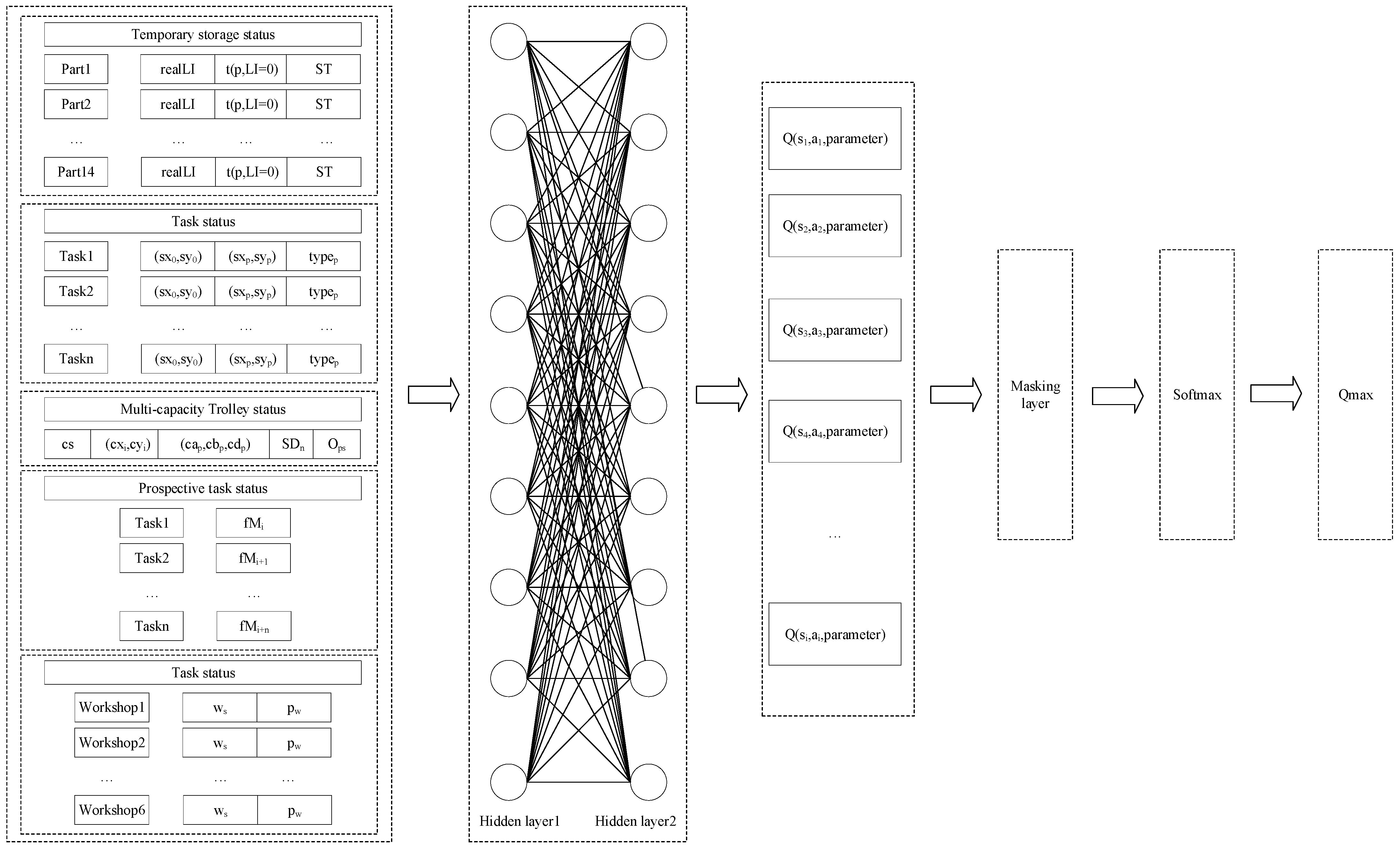
4. Neural Network Construction and Empirical Selection Method

When faced with a large-scale production system such as the automobile assembly line, due to the complex state of the production system and the large changes in the state space parameters, it is difficult for the agent to traverse each behavior under the massive production state. The feature extraction of input state information can be carried out by using a neural network; that is, the state space can be quasi-merged to extract effective key information, and the agent can be trained to obtain a better scheduling effect as much as possible. Since the state space of the workshop has been defined in detail above, there is no need to use the convolutional layer set in the original neural network of DQN to process the data. Therefore, the Q network structure consists of one input layer, two hidden layers, and one output layer (Figure 2).

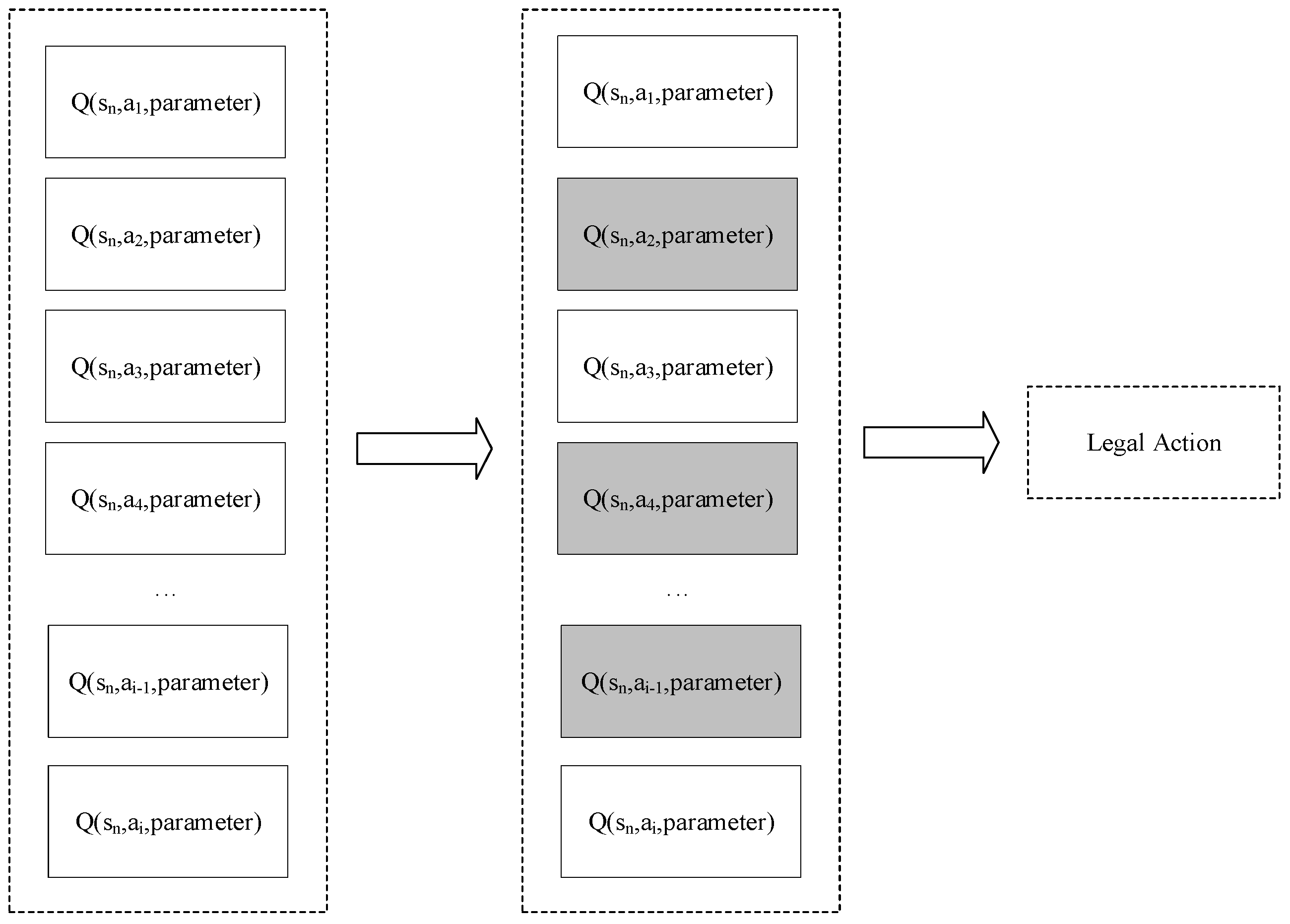
Because in the local workshop state, some actions $A_t$ output from the global consideration may not be legal in the current state, but these actions will also be output by the neural network. For illegal actions, a masking layer is added on the basis of the original neural network structure to mask the illegal actions and then output the Q value of other available actions, thereby improving the training speed of the algorithm and ensuring the stability of the algorithm during training (Figure 3). The neural network output layer will output the Q values of all actions in the action space and judge the actual executable action set through the local state. Elements are deleted, and then the softmax function is used to output the action with the largest Q value among all legal actions after screening.

In order to better alleviate the overestimation problem caused by bootstrapping, the update method of the neural network parameters is further modified, and the current action-value function $Q\left(s,a,\theta \right)$ is calculated by the evaluation Q network, and then the next action-value function $Q\left(s,a,\theta \right)$ is calculated by the target Q network. The optimal action-value function ${\mathrm{m}\mathrm{a}\mathrm{x}}_{{\mathrm{a}}^{\prime }}Q(s^{\prime },a^{\prime },{\theta }^{\prime })$ in a state is predicted, and finally, the Bellman equation is used to calculate the current action-value function $Q\left(s,a,{\theta }^{\prime }\right)$, the loss function $L\left(\theta \right)$ is calculated by comparing the difference between the target Q network and the evaluation Q network. The update formula is as follows:

$$Q\left(s,a,{\theta }^{\prime }\right)=\left\{\begin{array}{c}r, s=Terminal State\\ r+\gamma Q(s^{\prime },\underset{a}{\mathrm{argmax}}Q(s^{\prime },a,\theta ),{\theta }^{\prime })\end{array}\right.$$

(9)

$$L\left(\theta \right)=E(r+\gamma Q\left(s^{\prime },\underset{a}{\mathrm{argmax}}Q(s^{\prime },a,\theta ),{\theta }^{\prime }\right)-Q\left(s,a,\theta \right))$$

(10)

In the formula, $s$ represents the current state of the multi-load car; $s^{\prime }$ refers to the next state; $a$ is the action of the multi-capacity trolley; $r$ represents the environmental feedback reward obtained after the car performs the action; $\theta$ refers to the network parameter in the current state; ${\theta }^{\prime }$ refers to the network parameter in the next state; and $\gamma$ is the discount factor, indicating the discount degree of the future reward. Finally, $r$ and $s$ need to reach a terminal state to complete the update.

In order to reduce the correlation of data, an experience pool is established to store sample data for subsequent learning and use. When sampling and learning samples, batch sampling does not randomly sample but selects samples according to the priority of samples in the experience pool so that samples that need to be learned can be found more efficiently. According to TD error, we can obtain the learning priority p. The larger the TD error, the higher the priority p.

$$\mathrm{T}\mathrm{D} \mathrm{e}\mathrm{r}\mathrm{r}\mathrm{o}\mathrm{r}=r+\gamma Q\left(s^{\prime },\underset{a}{\mathrm{argmax}}Q(s^{\prime },a),\theta \right)-Q(s,a,\theta )$$

(11)

In order to judge the size of p, all samples need to be sorted according to p before each sampling, which takes a lot of time. This paper considers using the Sumtree method to process samples and adopts the prioritized experience replay (PER) mechanism to find samples with high priority so as to improve the learning efficiency of the model.

Considering the priority playback experience mechanism of the sample priority relationship, the loss function at this time is

$$L\left(\theta \right)=E(w_j(r+\gamma Q\left(s^{\prime },\underset{a}{\mathrm{argmax}}Q(s^{\prime },a,\theta ),{\theta }^{\prime }\right)-Q\left(s,a,\theta \right)))$$

(12)

where $w_j$ is the priority weight of the jth sample, obtained by TD-error error normalization; $N$ represents the total number of samples; $P\left(j\right)$ is the probability that sample j is selected; and $\beta$ is the degree to which prioritized experience replay affects the convergence result.

$$w_j={\displaystyle \frac{{N\ast P\left(j\right)}^{-\beta }}{{max}_i{w}_i}}$$

(13)

The complete algorithm process of the PER-DQN deep reinforcement learning method using priority experience replay is shown in Algorithm 1.

Algorithm 1: PER-DQN deep reinforcement learning algorithm based on priority experience replay

Input: number of iterations T, state space $n$, action space A, step size $N$, experience pool sampling weight coefficient $\beta$, decay parameter $\gamma$, exploration rate $\epsilon$, real Q network $\theta$, target Q network ${\theta }^{\prime }$, batch gradient descent sample number m, the target Q network parameter update frequency N, the number of Sumtree leaf nodes $S$ Initialize the neural network parameters, initialize the default data structure of experience playback Sumtree, and the priority $p_j$ of all Sumtree leaf nodes is 1 For episode = 1, m do   Obtain the current state $S_t$   For t = 1, T do      Randomly choose an action $a_t$ with probability $\epsilon$      Otherwise choose action $a_t=\underset{a}{\mathrm{argmax}}Q\left(S_t,a_t,\theta \right)$      Execute action $a_t$ and obtain new state $S_{t+1}$ and reward and punishment value R      Store in Sumtree $\left(S_t,a_t,r,S_{t+1}\right)$      Select m samples from Sumtree, the probability of each sample being sampled is based on $P\left(j\right)={\displaystyle \frac{p_j}{{\sum }_i\left(p_i\right)}}$, the loss function weight $w_j$, and calculate the target Q value                  $Q\left(s,a,{\theta }^{\prime }\right)=\left\{\begin{array}{c}r,s=TerminalState\\ r+\gamma Q(s^{\prime },\underset{a}{\mathrm{argmax}}Q\left(s^{\prime },a,\theta \right),{\theta }^{\prime })\end{array}\right.$    Calculate the loss function $L\left(\theta \right)=E(w_j(r+\gamma Q\left(s^{\prime },\underset{a}{\mathrm{argmax}}Q\left(s^{\prime },a,\theta \right),{\theta }^{\prime }\right)-Q\left(s,a,\theta \right)))$, update the Q network parameters using stochastic gradient descent    Recalculate the TD error of all samples and update the priorities of all nodes in the Sumtree    Set ${\theta }^{\prime }=\theta$ every N steps End for End for

5. Simulation Experiment Analysis

In this paper, the simulation model of the automobile mixed-model assembly line is built through the Arena simulation software (16.20.02), and the VBA module is used for secondary development to complete the interaction process between the scheduling method and the simulation model and realize the dynamic scheduling of the automobile assembly line. Compared with the common dynamic scheduling method based on a genetic algorithm, the performance of the dynamic scheduling method based on improved reinforcement learning proposed in this paper is verified. The parameter configuration of the simulation experiment is shown in

Table 1. Bill of materials, loading quantity of various parts, and distance from the material supermarket to each unloading point.

	${\mathbf{P}}_1$	${\mathbf{P}}_2$	${\mathbf{P}}_3$	${\mathbf{P}}_4$	${\mathbf{P}}_5$	${\mathbf{P}}_6$	${\mathbf{P}}_7$	${\mathbf{P}}_8$	${\mathbf{P}}_9$	${\mathbf{P}}_{10}$	${\mathbf{P}}_{11}$	${\mathbf{P}}_{12}$	${\mathbf{P}}_{13}$	${\mathbf{P}}_{14}$
${\mathrm{M}}_1$	1	1	1	1	0	0	1	1	0	0	1	0	0	1
${\mathrm{M}}_2$	1	0	0	0	1	1	1	0	1	0	0	1	0	1
${\mathrm{M}}_3$	1	0	0	0	1	0	1	1	0	1	0	0	1	0
$Q_p$	95	16	18	18	60	22	120	70	20	50	90	90	36	100
$\mathrm{D}\mathrm{i}\mathrm{s}/\mathrm{m}$	135	132	130	110	108	98	96	100	102	111	114	117	132	136

and

Table 2. Detailed parameter configuration in Arena simulation system.

Parameter	Value	Description
$\mathrm{P}\mathrm{T}$	3	Product model quantity
$\mathrm{P}\mathrm{R}$	(0.2, 0.5, 0.3)	Product ratio
$\mathrm{N}\mathrm{F}\mathrm{P}$	18	The number of forward-looking products
$\mathrm{S}\mathrm{T}$	6	Number of workstations
$NP$	14	Number of parts
$\mathrm{N}\mathrm{C}$	3	The maximum carrying capacity of the trolley
$\mathrm{C}\mathrm{T}\left(\mathrm{s}\right)$	72	Assembly beat
L (s)	37	Part loading time
R (s)	43	Part unloading time
v (m/s)	3	Trolley speed

, where P represents the part type, and M represents the product type. Since the work-in-progress movement between workstations on the conveyor belt is synchronous, the workstation that finishes assembly first must wait for the upstream workstation to complete the current assembly task before proceeding to assemble the next product. In order to make the whole assembly line continue, it is assumed that the assembly time CT of each workstation is 72 s. The simulation time is 100 h.

Considering the production characteristics of the automobile assembly line, this paper selects the following indicators to evaluate the performance of the scheduling method: average online inventory ALI, output TH, total handling distance TD, total number of shortages NS, and comprehensive cost CI. In actual production and manufacturing, the continuous and stable operation of the assembly line maximizes production efficiency and enables the achievement of maximum production capacity. Therefore, it is a priority to ensure that the material supply can arrive on time to ensure that there will be no out-of-stock stoppage. Secondly, since the facility layout of the assembly line has been completed in the early stage of production, which includes the planning of the line-side inventory capacity, the handling cost of the multi-capacity trolley is given priority over the line-side inventory within a certain range. Therefore, the weights of out-of-stock cost, distance cost, and inventory cost in workshop material-handling scheduling decrease in turn. The comprehensive cost is composed of the weighted stockout cost (TS), distance cost (TD), and inventory cost (ALI), with $a$, $b$, and $c$ representing the weights of the three, expressed as

$$CI=a\ast TS+b\ast TD+c\ast \sum {ALI}_p$$

(14)

Consider the order of magnitude relationship between out-of-stock time, handling distance, and average inventory level, assuming $a={10}^2,b={10}^2,c=1$. The simulation results are shown in

Table 3. Average online inventory of different methods for 100 h simulation.

Scheduling Method	Average Online Inventory ALI
	${\mathbf{P}}_1$	${\mathbf{P}}_2$	${\mathbf{P}}_3$	${\mathbf{P}}_4$	${\mathbf{P}}_5$	${\mathbf{P}}_6$	${\mathbf{P}}_7$	${\mathbf{P}}_8$	${\mathbf{P}}_9$	${\mathbf{P}}_{10}$	${\mathbf{P}}_{11}$	${\mathbf{P}}_{12}$	${\mathbf{P}}_{13}$	${\mathbf{P}}_{14}$
MBS-1	71	10	11	10	31	13	69	38	14	33	45	47	20	57
MBS-2	80	13	14	12	54	14	98	64	18	45	45	70	29	78
MBS-3	78	12	18	13	52	19	99	64	17	43	57	70	27	75
GA	50	10	10	11	32	14	66	39	15	28	28	49	23	58
RL	49	9	11	10	31	11	64	35	11	24	45	43	19	55
DQN	48	9	9	11	30	10	63	33	11	24	44	43	19	53
PRE-DQN	46	9	9	10	30	10	61	34	13	24	43	41	19	52

and

Table 4. Scheduling performance of different methods for 100 h simulation.

Scheduling Method	TH	TD	Sum (ALI)	NS	TS	CI
MBS-1	4992	205,394	469	3	272	20,567,069
MBS-2	4460	184,372	634	206	39,595	22,397,334
MBS-3	4453	183,383	644	229	39,858	22,324,744
GA	4993	97,911	433	2	187	9,810,233
RL	4995	95,248	417	0	0	9,525,217
DQN	4995	94,657	407	0	0	9,466,107
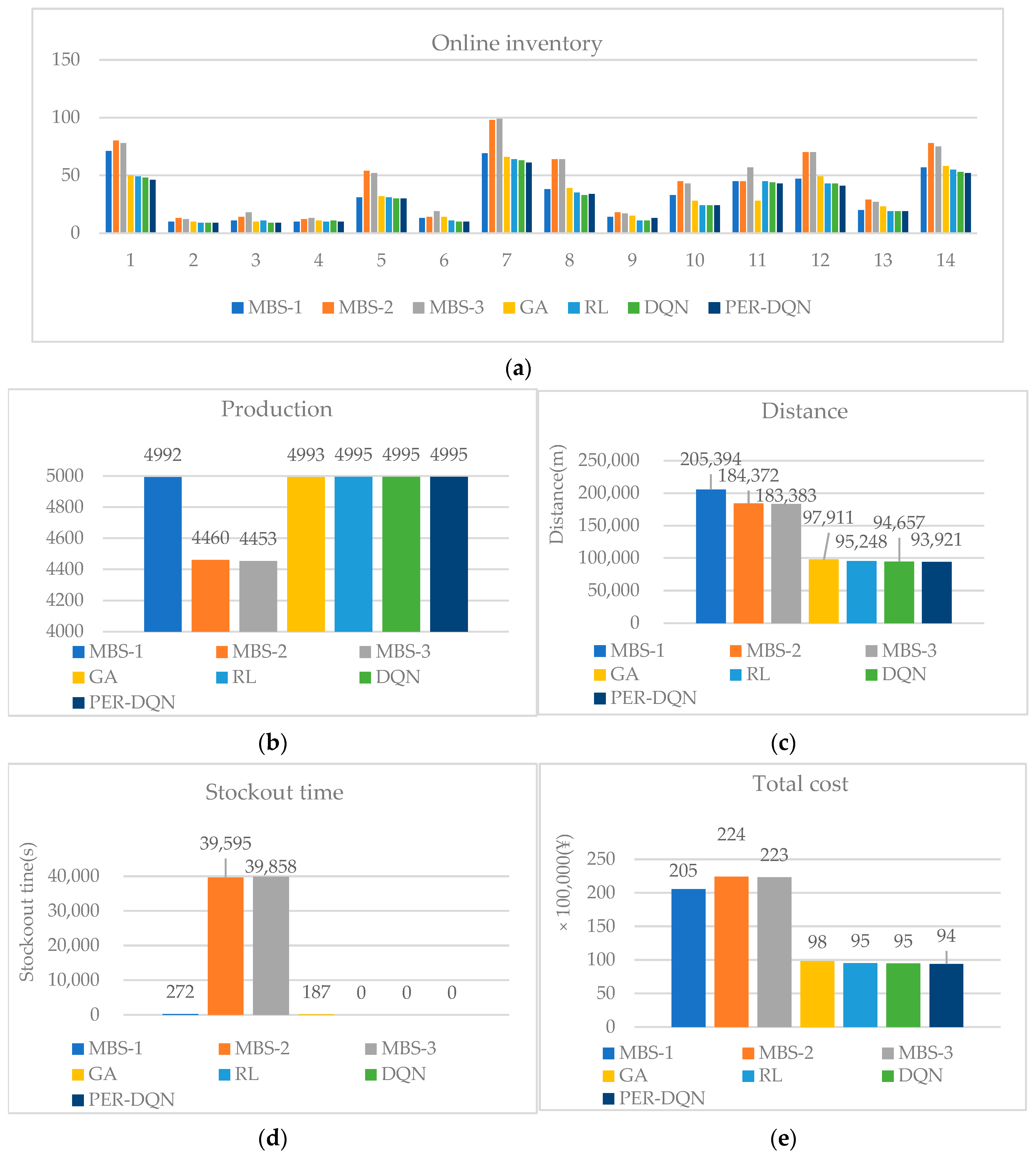
PER-DQN	4995	93,921	401	0	0	9,392,501

. In the 100 h simulation experiment, the deep reinforcement learning method was compared with the genetic algorithm in the intelligent algorithm, the reinforcement learning algorithm in the machine learning, and the traditional scheduling method minimum batch method (Figure 4). The minimum batch method can reduce the production preparation time and waiting time and improve production efficiency, but it has poor adaptability to the changing environment and demand. By simulating the process of natural selection and evolution, the genetic algorithm is insensitive to initial conditions and can find better solutions in various environments, but the convergence rate is relatively slow and may fall into local optimal solutions. DQN uses neural networks to learn Q-value functions, which can deal with high-dimensional state space and action space problems and has strong flexibility and applicability, but it may lead to overestimation problems and poor training results caused by data correlation. PER-DQN can give a higher sampling probability to important experiences so that these experiences are used more to improve learning efficiency and optimize data utilization. Since the maximum number of parts carried by the multi-capacity trolley set by the system is three types, three batch levels are set: MBS-1, MBS-2, and MBS-3. According to the results of the simulation experiment, the genetic algorithm GA, reinforcement learning RL, and deep reinforcement learning methods can all maximize the output, and there will be no shortage of goods, and the minimum batch and zero methods have the worst effect. Deep reinforcement learning DQN has a smaller transportation distance and lower comprehensive transportation cost. The PRE-DQN algorithm is better than DQN and has the best overall performance.

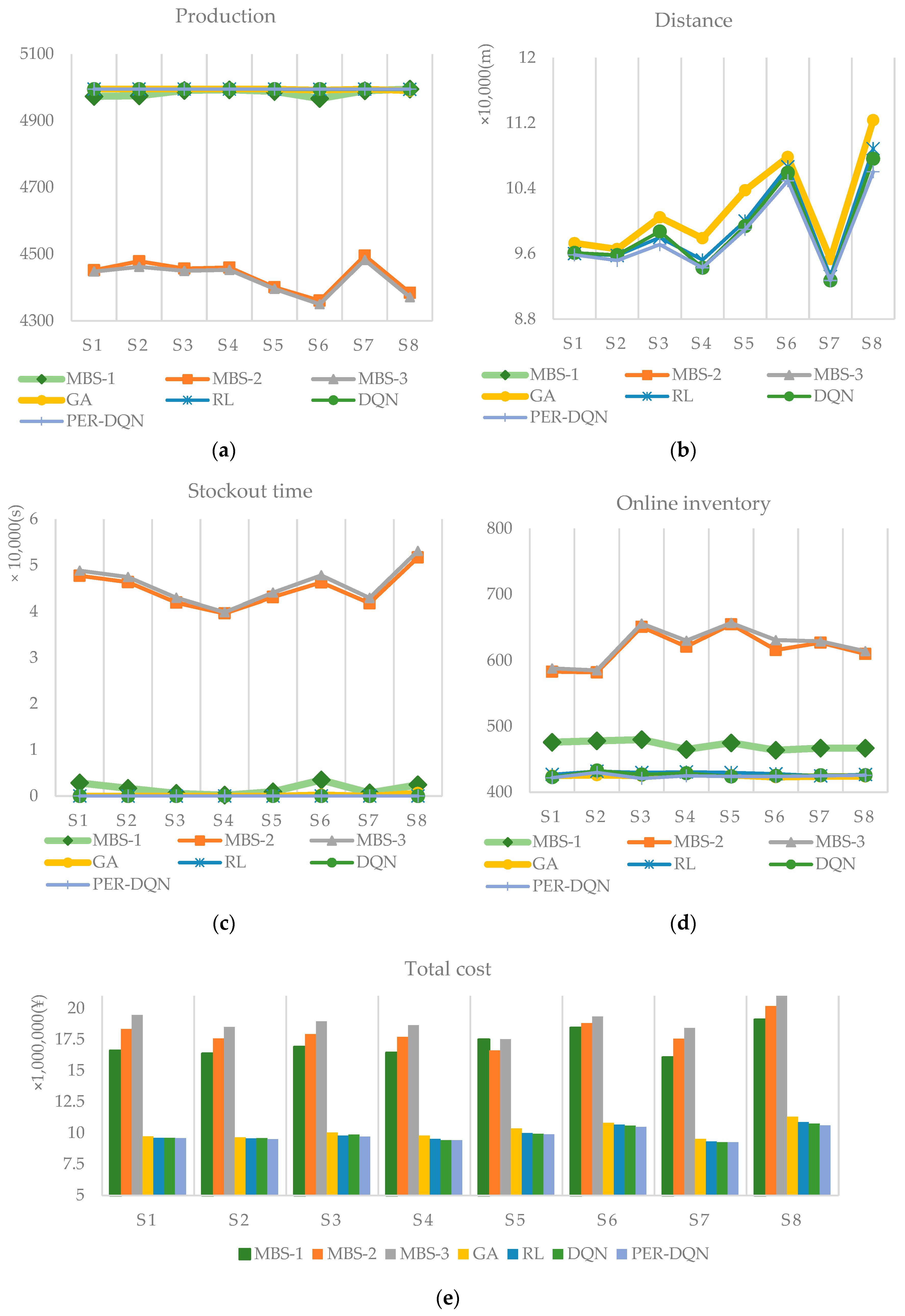
In actual production, the demand for automotive products will fluctuate and change due to the influence of individual market demand, which will correspondingly cause changes in the demand for materials on the assembly line. Therefore, we selected the product ratios of eight types of vehicles shown in

Table 5. The product ratios of 8 types of vehicles.

Group	M1	M2	M3
S1	0.1	0.8	0.1
S2	0.1	0.7	0.2
S3	0.2	0.6	0.2
S4	0.2	0.5	0.3
S5	0.3	0.4	0.3
S6	0.4	0.4	0.2
S7	0.2	0.4	0.4
S8	0.5	0.2	0.3

for sensitivity analysis to observe the performance of the scheduling method under different product ratios.

It can be seen from Figure 5 that the deep reinforcement learning method performs well in various scheduling performance indicators. The two deep reinforcement learning algorithms and the reinforcement learning RL algorithm have been running stably throughout the entire process without being out of stock, and the production lines have reached the maximum output. The genetic algorithm GA will be out of stock under the ratio of individual products. For the minimum batch transportation method, there will be out-of-stock situations in various batches, and the out-of-stock time will be longer. In most cases, the carrying distance of the deep reinforcement learning algorithm DQN is smaller than that of the reinforcement learning method RL, and the carrying distance of the PER-DQN algorithm is smaller than other algorithms. Although the average online library of DQN and PER-DQN algorithms is slightly higher than that of genetic algorithm GA in individual cases, overall, the PER-DQN algorithm method has the lowest total scheduling cost and the best performance. In the case of the same simulation parameter settings, the demand for each component is basically smooth throughout the simulation scheduling process. At this time, the online inventory is slightly higher, which may be due to the fact that there are more parts in one delivery, and the delivery distance is shorter than that of multiple deliveries of a single part. To sum up, the PER-DQN algorithm better balances various cost indicators, reduces the transportation distance of the trolley, and saves transportation costs. While ensuring the continuous and stable operation of the entire assembly system, it also takes advantage of the carrying advantages of the multi-capacity trolley. In this way, the optimization of the scheduling decision is realized overall.

The production order of the automobile assembly line can often be determined a few days before the execution of the production task, and there is sufficient time to adjust the assembly line scheduling system. However, for the workshop material-handling system, the material-handling task is issued internally by the production management system; the lead time for parts distribution may be only a few minutes or even shorter. According to the data, in the actual production process, the assembly line production cycle of General Motors in the United States is only a few tens of seconds, and the time spent on moving equipment during each handling process the driving time is usually a few minutes, and the possibility of changes in the initial scheduling information due to some random events during the dynamic scheduling process also needs to be considered. Therefore, the time to leave production information on the response line of the scheduling system is very precious. The real-time scheduling scheme of material handling must be able to respond quickly to changes in the entire production status and provide timely feedback to the system. Long-term optimization of the benefits of the production system so that the material information provided by the production system can be fully utilized to achieve multi-objective optimization.

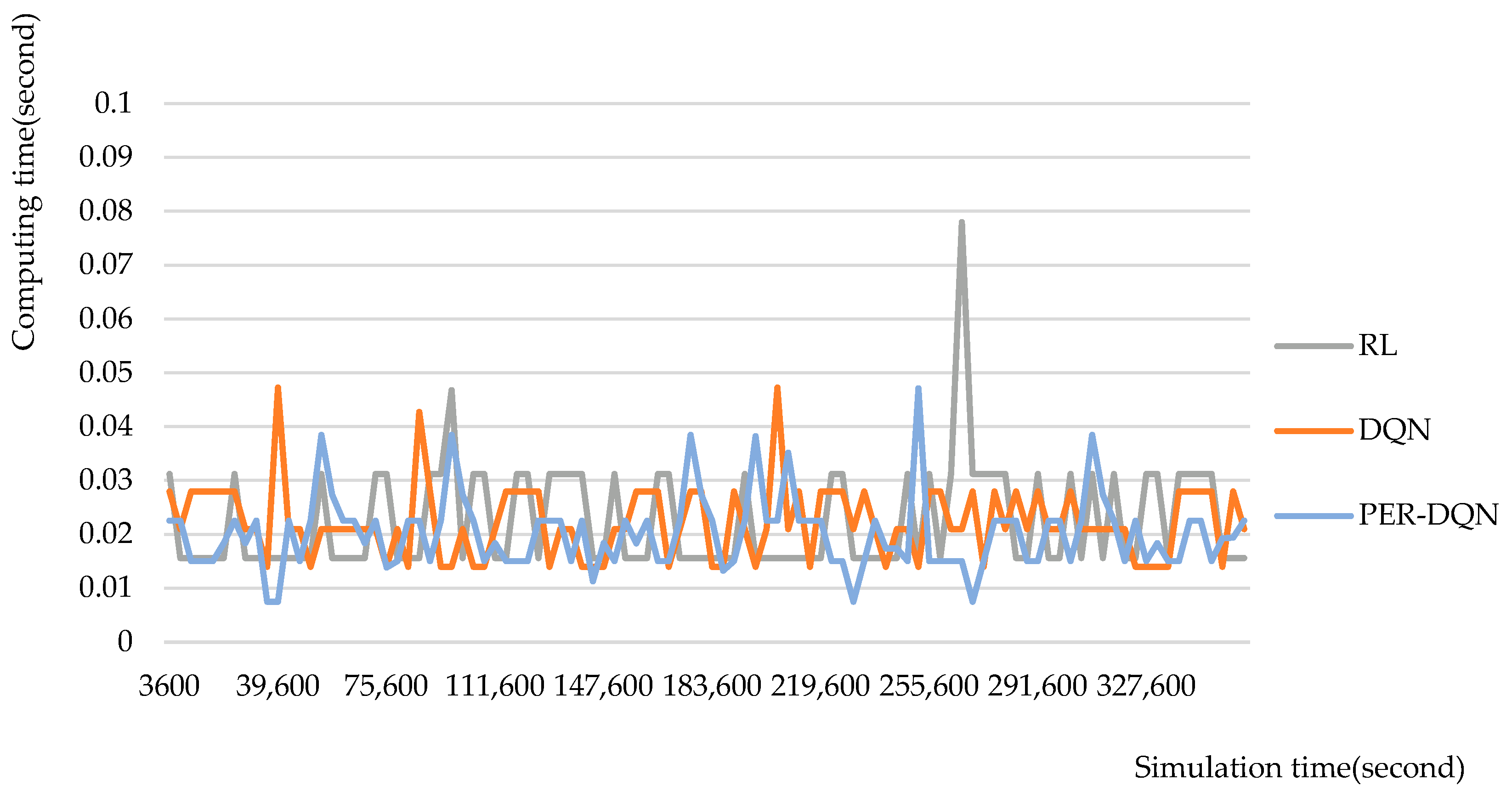
In order to verify the real-time response performance of the deep reinforcement learning scheduling methods DQN and PER-DQN, the RL method with better overall performance is selected for comparison, and the calculation time of the three scheduling methods are counted respectively. It can be seen from

Table 6. Comparison of calculation times for different scheduling methods.

	RL	DQN	PER-DQN
Average computing time	0.0225	0.0218	0.0201

that the calculation time consumed by the deep reinforcement learning scheduling method DQN and PER-DQN for a scheduling decision is slightly less than that of the reinforcement learning scheduling method RL. As shown in Figure 6, the time it takes for the deep reinforcement learning scheduling methods DQN and PER-DQN to make scheduling decisions during the entire 100 h simulation experiment is relatively stable. In most cases, the time spent by the two deep reinforcement learning algorithms is less than that of the reinforcement learning scheduling method (RL), with the calculation time of PER-DQN being the fastest. It can be seen that the deep reinforcement learning scheduling method can quickly make a decision on the material-handling system scheduling method that meets the real-time requirements in the actual production process. Compared to other scheduling methods, it shows better real-time responsiveness after training is completed.

6. Conclusions

In this paper, the deep reinforcement learning algorithm is applied to the material-handling scheduling problem in the workshop to realize the real-time dynamic scheduling of the material-handling system in the workshop. The neural network structure is modified according to the actual situation of the mixed-model assembly workshop to make it better applied to the material scheduling problem in the workshop. By changing the way neural network parameters are updated, the overestimation problem caused by DQN bootstrapping is reduced. Considering that the DQN learning algorithm may ignore some low-frequency but high-value samples during experience extraction, the Sumtree method is introduced to store sample experience, and the priority experience playback mechanism is adopted to form a real-time scheduling method for PER-DQN. Finally, through simulation verification, the PER-DQN scheduling method proposed in this paper can effectively avoid the out-of-stock shutdown problem caused by untimely delivery, ensure that parts can be transported to the corresponding workstations on time, and optimize the output, transport distance, and other indicators, while maintaining high output with low online inventory, the cost of material distribution is greatly reduced.

In the current field of assembly manufacturing, especially in enterprises in the new energy automotive, aerospace, and electronics industries, maintaining a high degree of operational flexibility to cope with uncertainties in the dynamic environment of the assembly shop has become an industry consensus. Furthermore, the principle of sustainability must be elevated to a strategic level of importance, especially in the context of new energy vehicles, such as electric cars, where the emphasis on energy conservation and emission reduction is paramount. In the actual manufacturing process, a variety of random events may occur, such as changes in product ratios due to market demands, machinery and equipment failures, or unexpected disruptions in the supply chain. To address these challenges, deep reinforcement learning technology has been introduced into the study of sustainable scheduling strategies, aiming to help enterprises achieve deep optimization of operational efficiency, significantly reduce energy consumption, and effectively promote long-term sustainability. This dual exploration of academia and practice not only provides a new perspective for the optimization of current manufacturing processes but also lays a solid theoretical and practical foundation for promoting the transition of the industry toward a greener, more sustainable future, especially in the realm of new energy vehicles and electric cars. In the future, combined with hyperparameter optimization is considered for further research.