


The Impacts of Urban Morphology on Urban Heat Islands in Housing Areas: The Case of Erzurum, Turkey
Abstract
1. Introduction
2. Materials and Methods
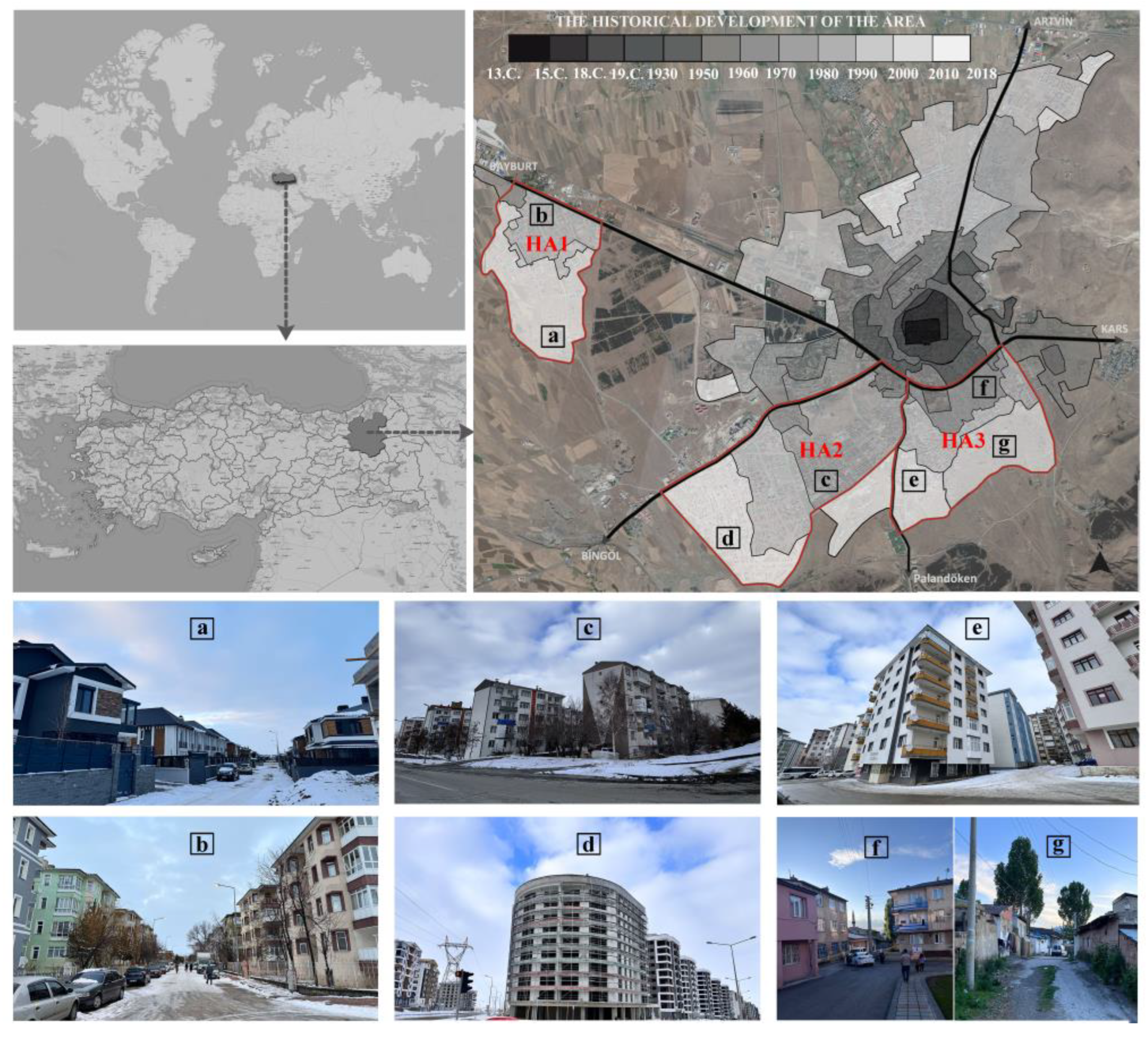
2.1. Study Area
2.2. Time Period
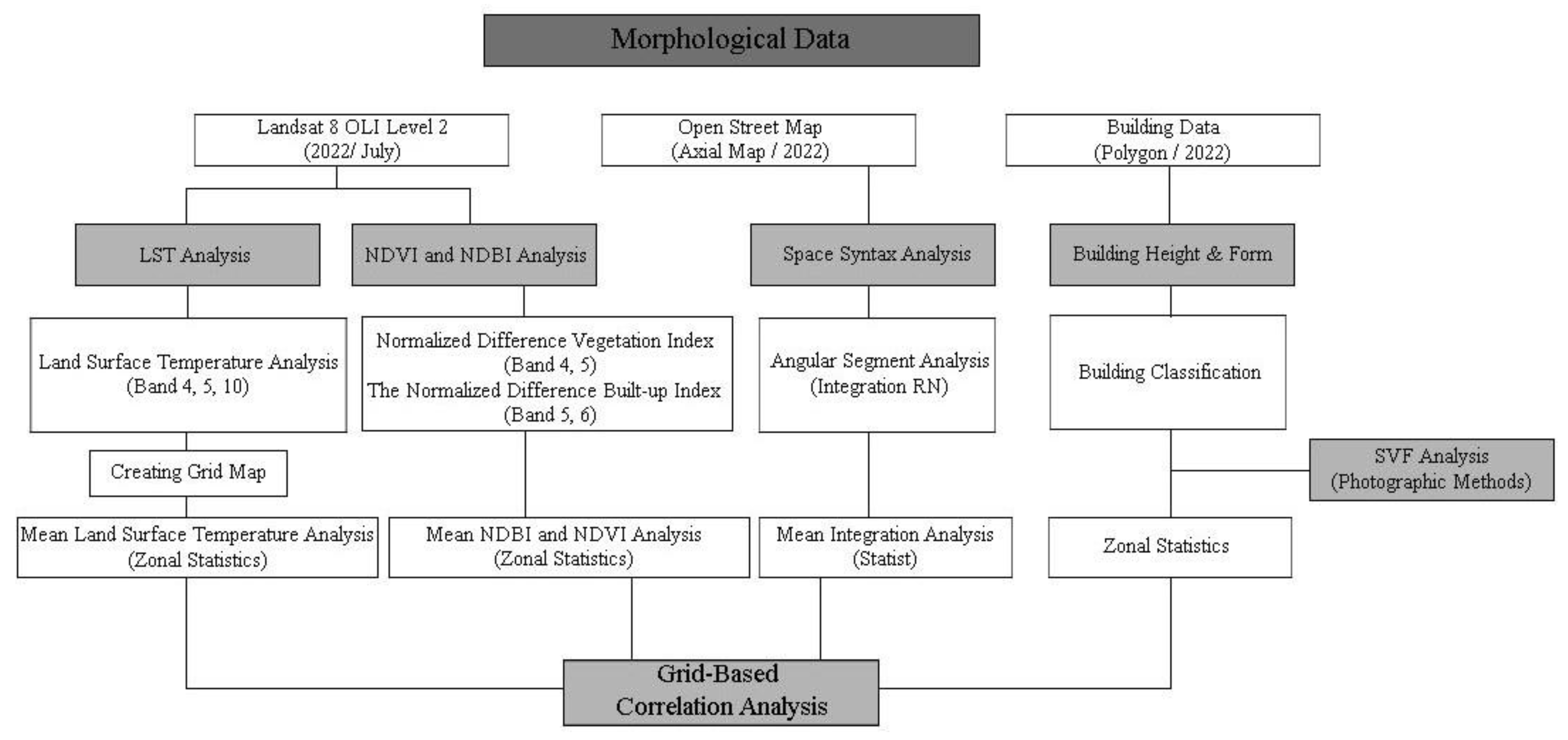
2.3. Materials
2.4. Methods
2.4.1. Land Surface Temperature Analysis
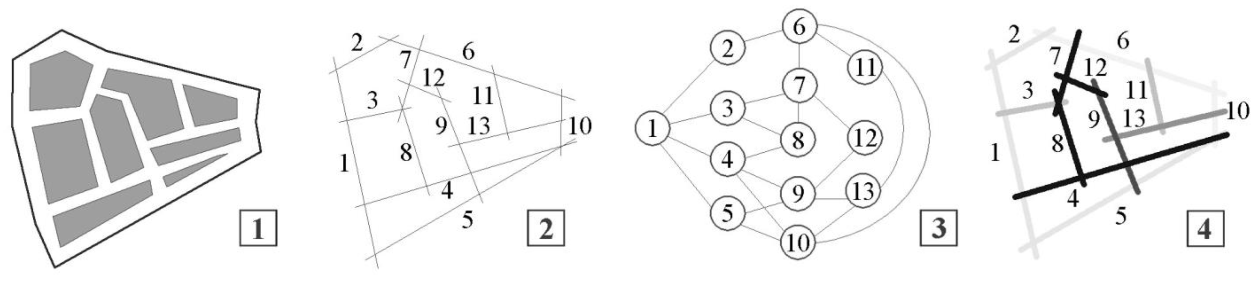
2.4.2. Space Syntax Analysis
- i.
- The street pattern (1) is transformed into an axial map (2), which is, albeit not precisely a graph, still a rudimentary representation.
- ii.
- The axial map (2) is transformed into a binary graph (3), referred to as a connectivity graph. This undirected graph consists of N nodes, the number of axial lines, and K links, representing intersections between pairs of axial lines.
- iii.
- Integration, a vital measure in Space Syntax, is determined through Equations (7) and (8). Within Space Syntax, the distance between two spaces is computed using a depth value [66]. In the computation of integration, Space Syntax typically calculates topological distance, which is defined as the minimum number of directional changes from each street segment to all others, commonly referred to as depth [65].
- iv.
- The integration of each node in the integration graph (3) is computed, and the colour-coded values are then mapped back onto the axial map (4), culminating in a final primitive-like colour-coded representation [65].
2.4.3. Sky View Factor Photographic Analysis
2.4.4. NDBI and NDVI Analysis
2.4.5. Statistical Analysis among Integration (Space Syntax), SVF, NDVI, NDBI, LST
3. Results
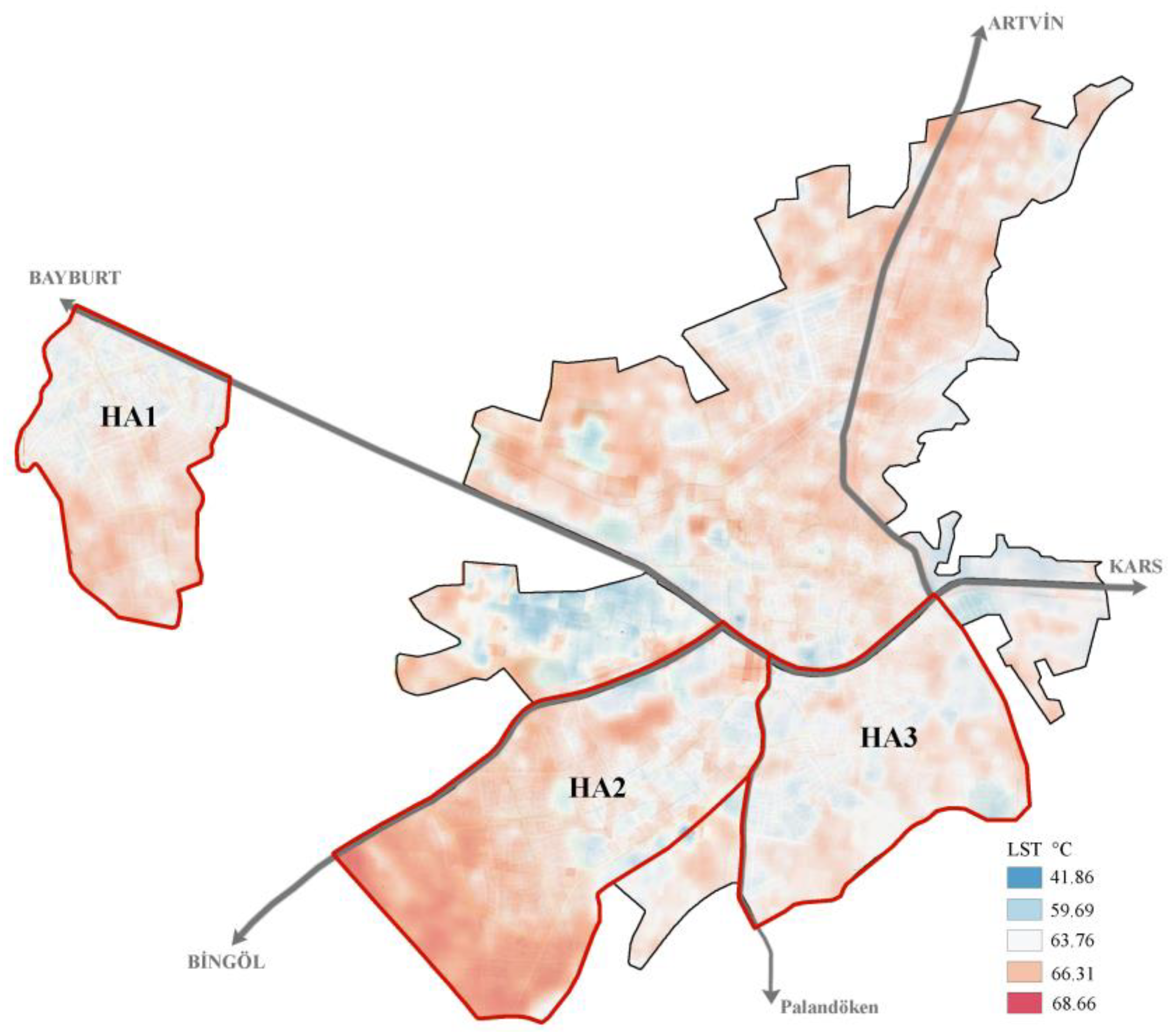
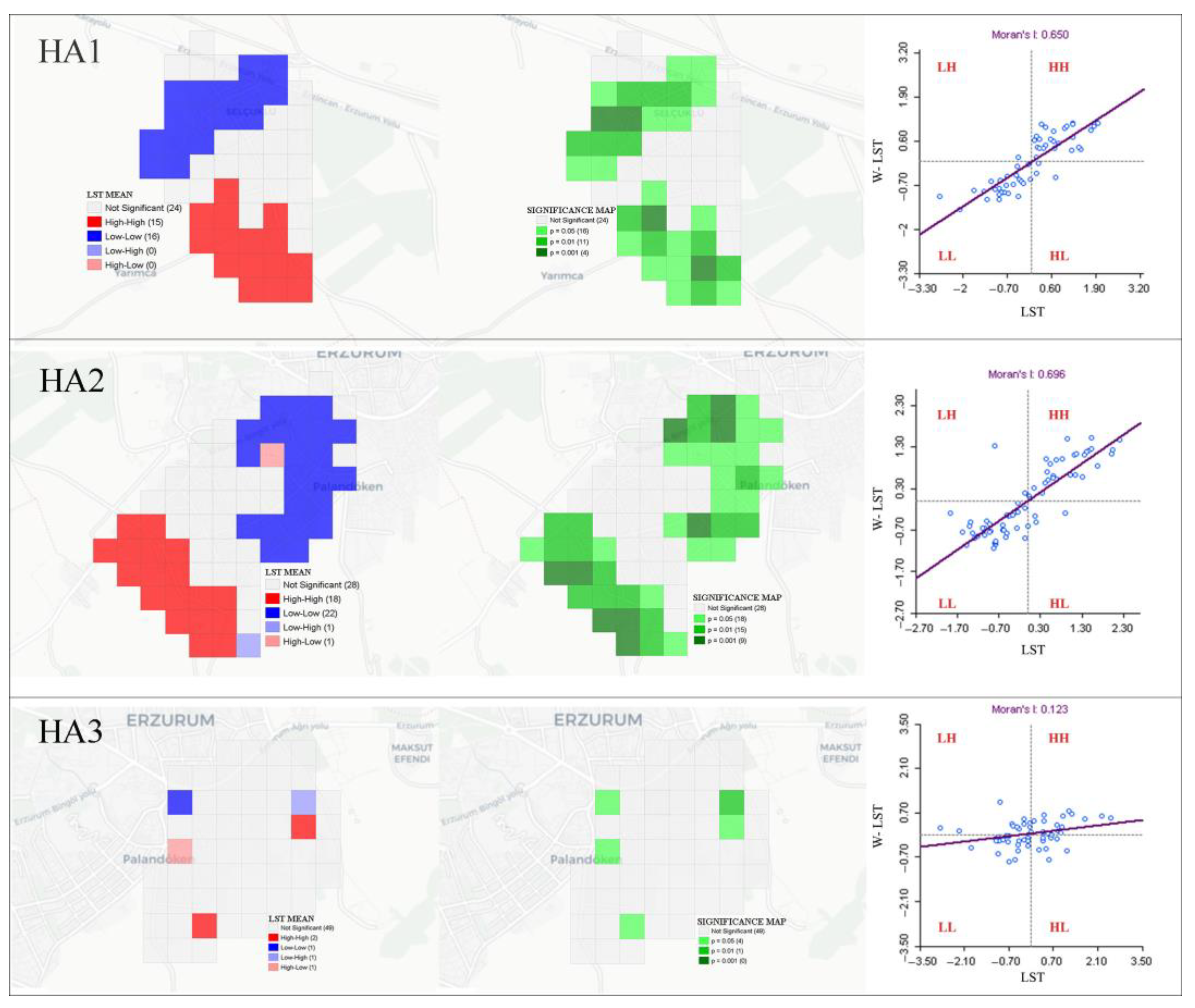
3.1. Results of Land Surface Temperature Analysis
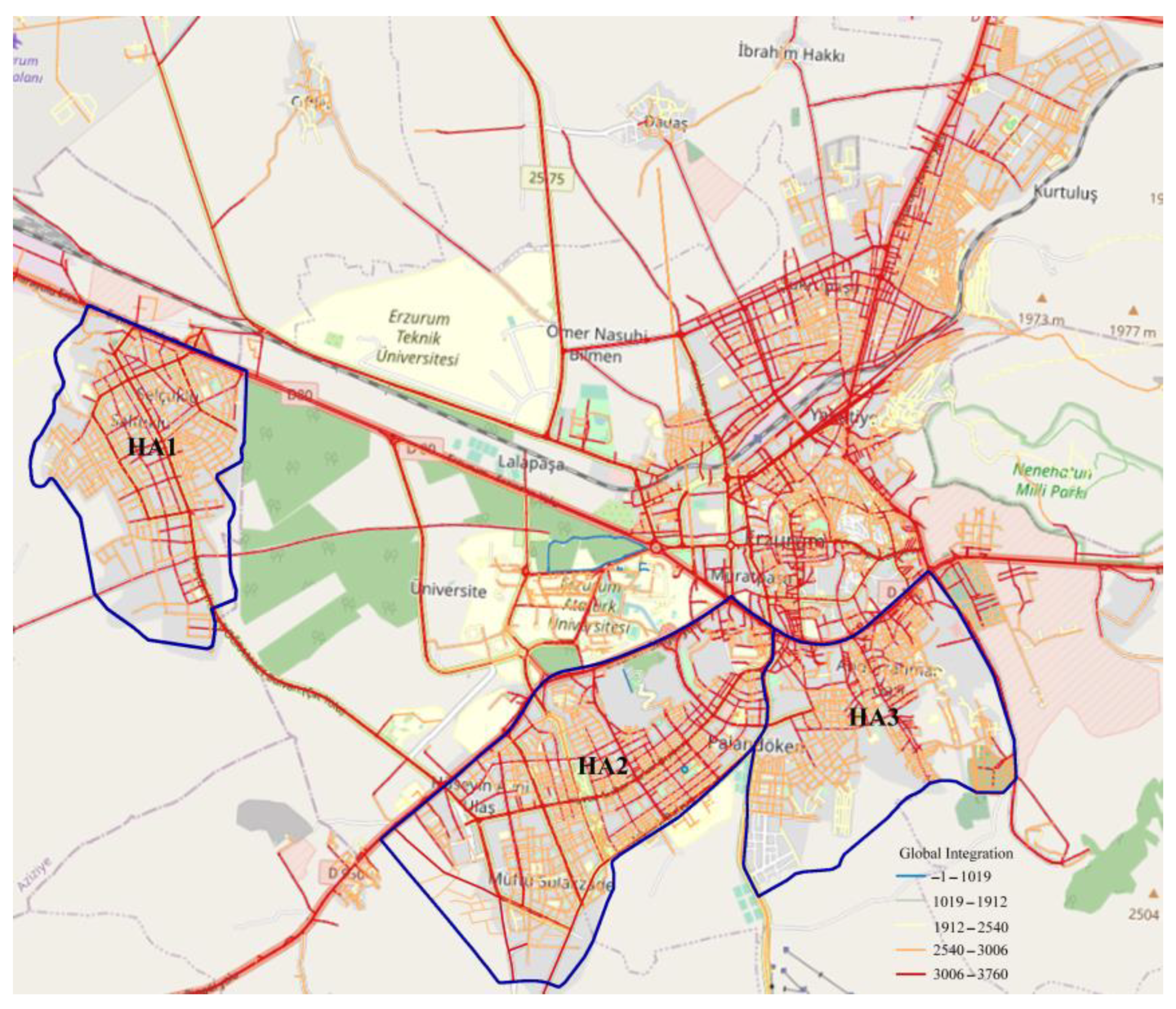
3.2. Results of Space Syntax Analysis
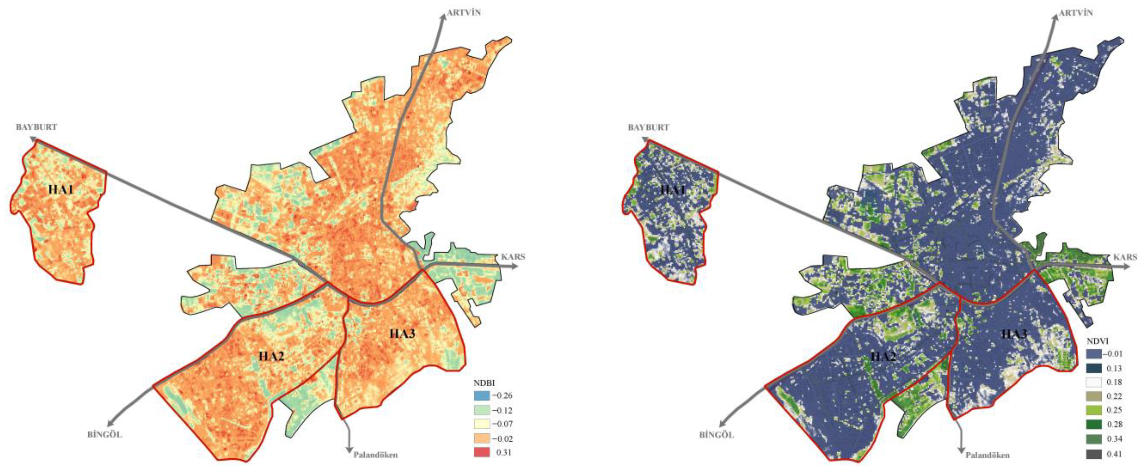
3.3. Results of NDVI and NDBI Analysis
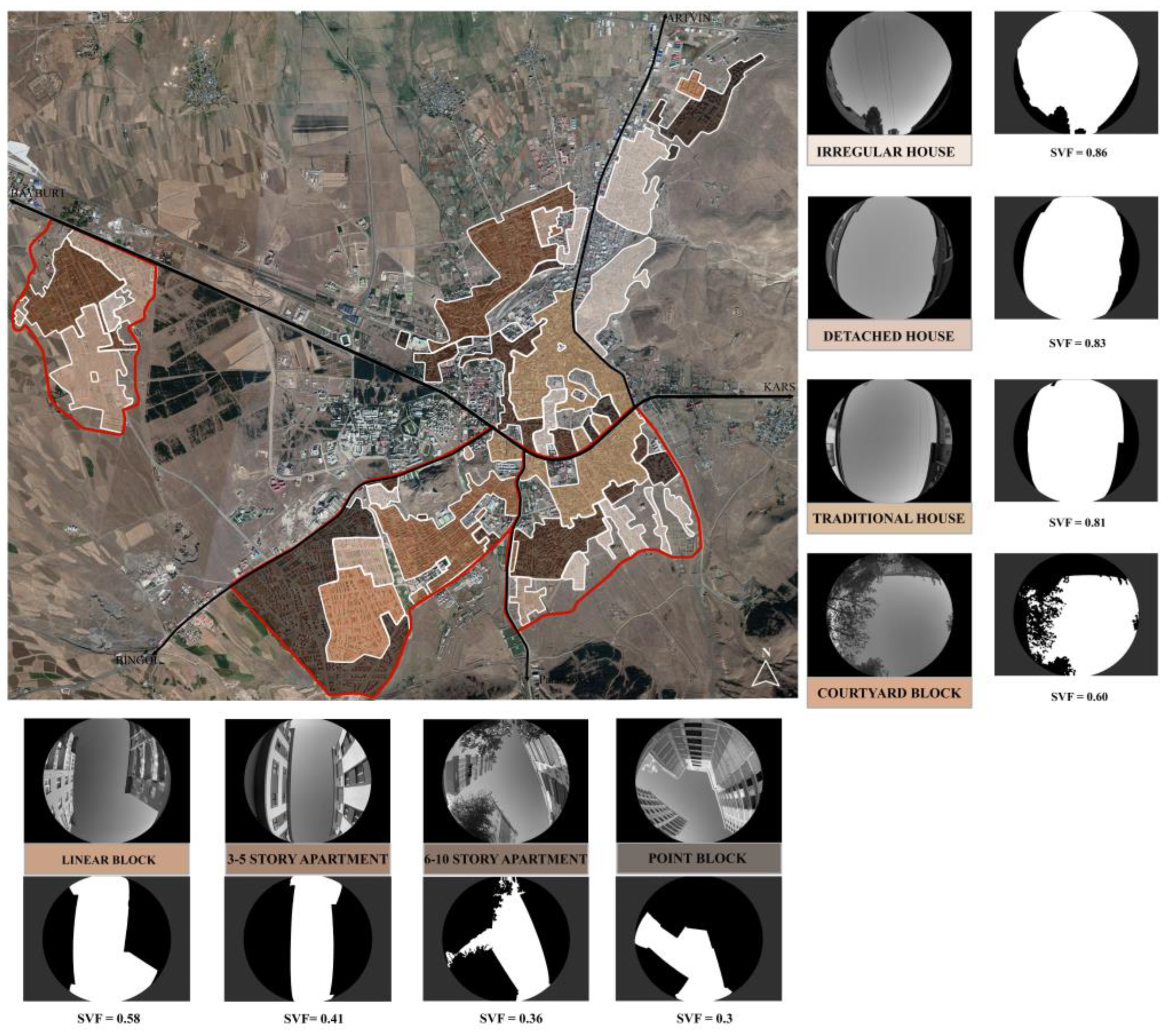
3.4. Results of Sky View Factor Photographic Analysis
3.5. Results of Correlation Analysis among Integration (Space Syntax), SVF, NDVI, NDBI and LST
4. Discussion
5. Conclusions
Author Contributions
Funding
Institutional Review Board Statement
Informed Consent Statement
Data Availability Statement
Conflicts of Interest
References
- Kovats, R.S.; Campbell-Lendrum, D.; Matthies, F. Climate change and human health: Estimating avoidable deaths and disease. Risk Anal. 2005, 25, 1409–1418. [Google Scholar] [CrossRef] [PubMed]
- Song, J.; Chen, W.; Zhang, J.; Huang, K.; Hou, B.; Prishchepov, A.V. Effects of building density on land surface temperature in China: Spatial patterns and determinants. Landsc. Urban Plan. 2020, 198, 103794. [Google Scholar] [CrossRef]
- Wang, W.; Liu, K.; Tang, R.; Wang, S. Remote sensing image-based analysis of the urban heat island effect in Shenzhen, China. Phys. Chem. Earth 2019, 110, 168–175. [Google Scholar] [CrossRef]
- Li, J.; Song, C.; Cao, L.; Zhu, F.; Meng, X.; Wu, J. Impacts of landscape structure on surface urban heat islands: A case study of Shanghai, China. Remote Sens. Environ. 2011, 115, 3249–3263. [Google Scholar] [CrossRef]
- Wei, Y.D.; Ye, X. Urbanization, urban land expansion and environmental change in China. Stoch. Environ. Res. Risk Assess. 2014, 28, 757–765. [Google Scholar] [CrossRef]
- Zhou, L.; Yuan, B.; Hu, F.; Wei, C.; Dang, X.; Sun, D. Understanding the effects of 2D/3D urban morphology on land surface temperature based on local climate zones. Build. Environ. 2022, 208, 108578. [Google Scholar] [CrossRef]
- Zhu, Z.; Wang, G.; Dong, J. Correlation analysis between land use/cover change and air pollutants—A case study in Wuyishan city. Energies 2019, 12, 2545. [Google Scholar] [CrossRef]
- Srivastava, A.; Shukla, S.; Singh, P.; Jha, P.K. Spatio-temporal dynamics of land use/cover and land surface temperature in Prayagraj city, India. Indoor Built Environ. 2023, 32, 1250–1268. [Google Scholar] [CrossRef]
- Fikfak, A.; Kosanović, S.; Konjar, M.; Grom, J.P.; Zbašnik-Senegačnik, M. The impact of morphological features on summer temperature variations on the example of two residential neighborhoods in Ljubljana, Slovenia. Sustainability 2017, 9, 122. [Google Scholar] [CrossRef]
- Arbuthnott, K.G.; Hajat, S. The health effects of hotter summers and heat waves in the population of the United Kingdom: A review of the evidence. Environ. Health 2017, 16, 119. [Google Scholar] [CrossRef]
- Adeyemi, A.; Ramoelo, A.; Cho, M.A.; Strydom, J. Spatio-temporal analysis of built-up impervious surface area and interplay with land surface temperature in Pretoria, South Africa. Geocarto Int. 2022, 37, 7618–7638. [Google Scholar] [CrossRef]
- Çağlak, S. Investigation the relationship between causes of death and thermal comfort conditions: The sample of Amasya Province. Int. J. Biometeorol. 2023, 67, 1353–1362. [Google Scholar] [CrossRef] [PubMed]
- Cheval, S.; Dumitrescu, A.; Irașoc, A.; Paraschiv, M.G.; Perry, M.; Ghent, D. MODIS-based climatology of the Surface Urban Heat Island at country scale (Romania). Urban Clim. 2022, 41, 101056. [Google Scholar] [CrossRef]
- Schlünzen, K.H.; Grimmond, S.; Baklanov, A. Development of the CL-UHI. In Guidance to Measuring, Modelling and Monitoring the Canopy Layer Urban Heat Island; WMO: Geneva, Switzerland, 2023; pp. 7–12. [Google Scholar] [CrossRef]
- Chew, L.W.; Norford, L.K. Pedestrian-level wind speed enhancement in urban street canyons with void decks. Build. Environ. 2018, 146, 64–76. [Google Scholar] [CrossRef]
- Hofman, J.; Castanheiro, A.; Nuyts, G.; Joosen, S.; Spassov, S.; Blust, R.; Wael, K.; Lenaerts, S.; Samson, R. Impact of urban street canyon architecture on local atmospheric pollutant levels and magneto-chemical PM10 composition: An experimental study in Antwerp, Belgium. Sci. Total Environ. 2020, 712, 135534. [Google Scholar] [CrossRef]
- Karimimoshaver, M.; Khalvandi, R.; Khalvandi, M. The effect of urban morphology on heat accumulation in urban street canyons and mitigation approach. Sustain. Cities Soc. 2021, 73, 103127. [Google Scholar] [CrossRef]
- Zhou, D.; Xiao, J.; Bonafoni, S.; Berger, C.; Deilami, K.; Zhou, Y.; Frolking, S.; Yao, R.; Qiao, Z.; Sobrino, J.A. Satellite remote sensing of surface urban heat islands: Progress, challenges, and perspectives. Remote Sens. 2018, 11, 48. [Google Scholar] [CrossRef]
- Zhou, X.; Chen, H. Impact of urbanization-related land use land cover changes and urban morphology changes on the urban heat island phenomenon. Sci. Total Environ. 2018, 635, 1467–1476. [Google Scholar] [CrossRef]
- He, B.J.; Ding, L.; Prasad, D. Relationships among local-scale urban morphology, urban ventilation, urban heat island and outdoor thermal comfort under sea breeze influence. Sustain. Cities Soc. 2020, 60, 102289. [Google Scholar] [CrossRef]
- Badaro-Saliba, N.; Adjizian-Gerard, J.; Zaarour, R.; Najjar, G. LCZ scheme for assessing Urban Heat Island intensity in a complex urban area (Beirut, Lebanon). Urban Clim. 2021, 37, 100846. [Google Scholar] [CrossRef]
- Hassan, T.; Zhang, J.; Prodhan, F.A.; Pangali Sharma, T.P.; Bashir, B. Surface urban heat islands dynamics in response to LULC and vegetation across South Asia (2000–2019). Remote Sens. 2021, 13, 3177. [Google Scholar] [CrossRef]
- Faisal, A.A.; Kafy, A.A.; Al Rakib, A.; Akter, K.S.; Jahir, D.M.A.; Sikdar, M.S.; Ashrafi, T.J.; Mallik, S.; Rahman, M.M. Assessing and predicting land use/land cover, land surface temperature and urban thermal field variance index using Landsat imagery for Dhaka Metropolitan area. Environ. Chall. 2021, 4, 100192. [Google Scholar] [CrossRef]
- Liu, X.; Ming, Y.; Liu, Y.; Yue, W.; Han, G. Influences of landform and urban form factors on urban heat island: Comparative case study between Chengdu and Chongqing. Sci. Total Environ. 2022, 820, 153395. [Google Scholar] [CrossRef] [PubMed]
- Allegrini, J.; Carmeliet, J. Simulations of local heat islands in Zürich with coupled CFD and building energy models. Urban Clim. 2018, 24, 340–359. [Google Scholar] [CrossRef]
- Guo, C.; Buccolieri, R.; Gao, Z. Characterizing the morphology of real street models and modelling its effect on thermal environment. Energy Build. 2019, 203, 109433. [Google Scholar] [CrossRef]
- Liu, B.; Guo, X.; Jiang, J. How Urban Morphology Relates to the Urban Heat Island Effect: A Multi-Indicator Study. Sustainability 2023, 15, 10787. [Google Scholar] [CrossRef]
- Seo, K.W.; Lee, S. Oxcart route in the city: Tracking the urbanization process of an agricultural village in Korea. Sustainability 2019, 11, 2153. [Google Scholar] [CrossRef]
- Wang, X.; Yao, X.; Shao, H.; Bai, T.; Xu, Y.; Tian, G.; Fekete, A.; Kollányi, L. Land Use Quality Assessment and Exploration of the Driving Forces Based on Location: A Case Study in Luohe City, China. Land 2023, 12, 257. [Google Scholar] [CrossRef]
- Nasehi, S.; Yavari, A.; Salehi, E.; Emmanuel, R. Role of local climate zone and space syntax on land surface temperature (case study: Tehran). Urban Clim. 2022, 45, 101245. [Google Scholar] [CrossRef]
- Soltanifard, H.; Aliabadi, K. Impact of urban spatial configuration on land surface temperature and urban heat islands: A case study of Mashhad, Iran. Theor. Appl. Climatol. 2019, 137, 2889–2903. [Google Scholar] [CrossRef]
- Hillier, B.; Turner, A.; Yang, T.; Park, H.T. Metric and topo-geometric properties of urban street networks: Some convergences, divergences and new results. In Proceedings of the 6th International Space Syntax Symposium 2007, Istanbul, Turkey, 12–15 June 2007; p. 22. [Google Scholar]
- Scarano, M.; Sobrino, J.A. On the relationship between the sky view factor and the land surface temperature derived by Landsat-8 images in Bari, Italy. Int. J. Remote Sens. 2015, 36, 4820–4835. [Google Scholar] [CrossRef]
- Hu, Y.; Dai, Z.; Guldmann, J.M. Modeling the impact of 2D/3D urban indicators on the urban heat island over different seasons: A boosted regression tree approach. J. Environ. Manag. 2020, 266, 110424. [Google Scholar] [CrossRef]
- Zhu, Z.; Shen, Y.; Fu, W.; Zheng, D.; Huang, P.; Li, J.; Lan, Y.; Chen, Z.; Liu, A.; Xu, X.; et al. How does 2D and 3D of urban morphology affect the seasonal land surface temperature in Island City? A block-scale perspective. Ecol. Indic. 2023, 150, 110221. [Google Scholar] [CrossRef] [PubMed]
- Susca, T.; Gaffin, S.R.; Dell’Osso, G.R. Positive effects of vegetation: Urban heat island and green roofs. Environ. Pollut. 2011, 159, 2119–2126. [Google Scholar] [CrossRef]
- Li, X.; Zhou, W.; Ouyang, Z. Relationship between land surface temperature and spatial pattern of greenspace: What are the effects of spatial resolution? Landsc. Urban Plan. 2013, 114, 1–8. [Google Scholar] [CrossRef]
- Feyisa, G.L.; Dons, K.; Meilby, H. Efficiency of parks in mitigating urban heat island effect: An example from Addis Ababa. Landsc. Urban Plan. 2014, 123, 87–95. [Google Scholar] [CrossRef]
- Dos Santos, A.R.; de Oliveira, F.S.; da Silva, A.G.; Gleriani, J.M.; Gonçalves, W.; Moreira, G.L.; Silva, F.G.; Branco, E.R.F.; Moura, M.M.; da Silva, R.G.; et al. Spatial and temporal distribution of urban heat islands. Sci. Total Environ. 2017, 605, 946–956. [Google Scholar] [CrossRef]
- Karakuş, C.B. The impact of land use/land cover (LULC) changes on land surface temperature in Sivas City Center and its surroundings and assessment of Urban Heat Island. Asia-Pac. J. Atmos. Sci. 2019, 55, 669–684. [Google Scholar] [CrossRef]
- Hua, L.; Zhang, X.; Nie, Q.; Sun, F.; Tang, L. The impacts of the expansion of urban impervious surfaces on urban heat islands in a coastal city in China. Sustainability 2020, 12, 475. [Google Scholar] [CrossRef]
- Yang, C.; Yan, F.; Zhang, S. Comparison of land surface and air temperatures for quantifying summer and winter urban heat island in a snow climate city. J. Environ. Manag. 2020, 265, 110563. [Google Scholar] [CrossRef]
- Pakarnseree, R.; Chunkao, K.; Bualert, S. Physical characteristics of Bangkok and its urban heat island phenomenon. Build Environ. 2018, 143, 561–569. [Google Scholar] [CrossRef]
- He, T.; Zhou, R.; Ma, Q.; Li, C.; Liu, D.; Fang, X.; Yina, H.; Gao, J. Quantifying the effects of urban development intensity on the surface urban heat island across building climate zones. Appl. Geogr. 2023, 158, 103052. [Google Scholar] [CrossRef]
- Sun, F.; Liu, M.; Wang, Y.; Wang, H.; Che, Y. The effects of 3D architectural patterns on the urban surface temperature at a neighborhood scale: Relative contributions and marginal effects. J. Clean. Prod. 2020, 258, 120706. [Google Scholar] [CrossRef]
- Peng, S.; Piao, S.; Ciais, P.; Friedlingstein, P.; Ottle, C.; Bréon, F.M.; Nan, H.; Zhou, L.; Myneni, R.B. Surface urban heat island across 419 global big cities. Environ. Sci. Technol. 2012, 46, 696–703. [Google Scholar] [CrossRef]
- Clinton, N.; Gong, P. MODIS detected surface urban heat islands and sinks: Global locations and controls. Remote Sens. Environ. 2013, 134, 294–304. [Google Scholar] [CrossRef]
- Li, X.; Zhou, Y.; Asrar, G.R.; Imhoff, M.; Li, X. The surface urban heat island response to urban expansion: A panel analysis for the conterminous United States. Sci. Total Environ. 2017, 605, 426–435. [Google Scholar] [CrossRef]
- Dai, Z.; Guldmann, J.M.; Hu, Y. Spatial regression models of park and land-use impacts on the urban heat island in central Beijing. Sci. Total Environ. 2018, 626, 1136–1147. [Google Scholar] [CrossRef] [PubMed]
- Huang, Q.; Lu, Y. Urban heat island research from 1991 to 2015: A bibliometric analysis. Theor. Appl. Climatol. 2018, 131, 1055–1067. [Google Scholar] [CrossRef]
- Dursun, D.; Güller, C. Relationship between child and urban space: Accessibility and areal efficiency analysis of playgrounds in Erzurum. J. Grad. Sch. Nat. Appl. Sci. Mehmet Akif Ersoy Univ. 2019, 10, 11–27. [Google Scholar] [CrossRef]
- Available online: https://atlas.harita.gov.tr (accessed on 1 December 2023).
- Lee, J.; Lee, Y.G.; Kim, B.J. Analysis of the thermal environment around an urban green area in Seoul, Korea using Climate Analysis Seoul (CAS). Atmosphere 2016, 26, 413–421. [Google Scholar] [CrossRef]
- Park, J.H.; Cho, G.H. Examining the association between physical characteristics of green space and land surface temperature: A case study of Ulsan, Korea. Sustainability 2016, 8, 777. [Google Scholar] [CrossRef]
- Srivanit, M.; Kazunori, H. The influence of urban morphology indicators on summer diurnal range of urban climate in Bangkok metropolitan area, Thailand. Int. J. Civ. Environ. Eng. 2011, 11, 34–46. [Google Scholar]
- Lee, K.; Kim, Y.; Sung, H.C.; Kim, S.H.; Jeon, S.W. Surface urban heat island in South Korea’s new towns with different urban planning. E Environ. Monit. Assess. 2022, 194, 360. [Google Scholar] [CrossRef] [PubMed]
- Thanvisitthpon, N. Statistically Validated Urban Heat Island Risk Indicators for UHI Susceptibility Assessment. Int. J. Environ. Res. Public Health 2023, 20, 1172. [Google Scholar] [CrossRef] [PubMed]
- Yu, X.; Guo, X.; Wu, Z. Land surface temperature retrieval from Landsat 8 TIRS—Comparison between radiative transfer equation-based method, split window algorithm and single channel method. Remote Sens. 2014, 6, 9829–9852. [Google Scholar] [CrossRef]
- Kim, J.; Lee, D.K.; Brown, R.D.; Kim, S.; Kim, J.H.; Sung, S. The effect of extremely low sky view factor on land surface temperatures in urban residential areas. Sustain. Cities Soc. 2022, 80, 103799. [Google Scholar] [CrossRef]
- Liu, J.; Feng, Q.; Gong, J.; Zhou, J.; Liang, J.; Li, Y. Winter wheat mapping using a random forest classifier combined with multi-temporal and multi-sensor data. Int. J. Digit. Earth 2018, 11, 783–802. [Google Scholar] [CrossRef]
- Nadizadeh Shorabeh, S.; Hamzeh, S.; Zanganeh Shahraki, S.; Firozjaei, M.K.; Jokar Arsanjani, J. Modelling the intensity of surface urban heat island and predicting the emerging patterns: Landsat multi-temporal images and Tehran as case study. Int. J. Remote Sens. 2020, 41, 7400–7426. [Google Scholar] [CrossRef]
- Hillier, B. Space is the machine: A configurational theory of architecture. J. Urban Des. 2007, 3, 333–335. [Google Scholar]
- Liu, X.; Jiang, B. Defining and generating axial lines from street center lines for better understanding of urban morphologies. Int. J. Geogr. Inf. Syst. 2012, 26, 1521–1532. [Google Scholar] [CrossRef]
- Johnsson, C.; Camporeale, R. Exploring Space Syntax Integration at Public Transport Hubs and Public Squares Using Drone Footage. Appl. Sci. 2022, 12, 6515. [Google Scholar] [CrossRef]
- Crucitti, P.; Latora, V.; Porta, S. Centrality in networks of urban streets. Chaos 2006, 16, 015113. [Google Scholar] [CrossRef] [PubMed]
- Xia, C.; Zhang, A.; Wang, H.; Yeh, A.G. Predicting the expansion of urban boundary using space syntax and multivariate regression model. Habitat Int. 2019, 86, 126–134. [Google Scholar] [CrossRef]
- Chapman, L.; Thornes, J.E. Real-time sky-view factor calculation and approximation. J. Atmos. Ocean. Technol. 2004, 21, 730–741. [Google Scholar] [CrossRef]
- Grimmond, C.S.B.; Potter, S.K.; Zutter, H.N.; Souch, C. Rapid methods to estimate sky-view factors applied to urban areas. Int. J. Climatol. 2001, 21, 903–913. [Google Scholar] [CrossRef]
- Shaker, R.R.; Drezner, T.D. A New Technique for Predicting the Sky-View Factor for Urban Heat Island Assessment. Geogr. Bull. 2010, 51, 85–96. [Google Scholar]
- Svensson, M.K. Sky view factor analysis–implications for urban air temperature differences. Meteorol. Appl. 2004, 11, 201–211. [Google Scholar] [CrossRef]
- Debbage, N. Sky-view factor estimation: A case study of Athens, Georgia. Geogr. Bull. 2013, 54, 49. [Google Scholar]
- Halder, B.; Bandyopadhyay, J.; Banik, P. Monitoring the effect of urban development on urban heat island based on remote sensing and geo-spatial approach in Kolkata and adjacent areas, India. Sustain. Cities Soc. 2021, 74, 103186. [Google Scholar] [CrossRef]
- Hidalgo-García, D.; Arco-Díaz, J. Modeling the Surface Urban Heat Island (SUHI) to study of its relationship with variations in the thermal field and with the indices of land use in the metropolitan area of Granada (Spain). Sustain. Cities Soc. 2022, 87, 104166. [Google Scholar] [CrossRef]
- Mansour, K.; Aziz, M.A.; Hashim, S.; Effat, H. Impact of anthropogenic activities on urban heat islands in major cities of El-Minya Governorate, Egypt. Egypt. J. Remote Sens. Space Sci. 2022, 25, 609–620. [Google Scholar] [CrossRef]
- Kshetri, T. Ndvi, ndbi & ndwi calculation using landsat 7, 8. GeoWorld 2018, 2, 32–34. [Google Scholar]
- Wang, J.; Rich, P.M.; Price, K.P. Temporal responses of NDVI to precipitation and temperature in the central Great Plains, USA. Int. J. Remote Sens. 2003, 24, 2345–2364. [Google Scholar] [CrossRef]
- Pettorelli, N.; Vik, J.O.; Mysterud, A.; Gaillard, J.M.; Tucker, C.J.; Stenseth, N.C. Using the satellite-derived NDVI to assess ecological responses to environmental change. Trends Ecol. Evol. 2005, 20, 503–510. [Google Scholar] [CrossRef]
- Huang, S.; Tang, L.; Hupy, J.P.; Wang, Y.; Shao, G. A commentary review on the use of normalized difference vegetation index (NDVI) in the era of popular remote sensing. J. For. Res. 2021, 32, 1–6. [Google Scholar] [CrossRef]
- Li, S.; Xu, L.; Jing, Y.; Yin, H.; Li, X.; Guan, X. High-quality vegetation index product generation: A review of NDVI time series reconstruction techniques. Int. J. Appl. Earth Obs. Geoinf. 2021, 105, 102640. [Google Scholar] [CrossRef]
- Zha, Y.; Gao, J.; Ni, S. Use of normalized difference built-up index in automatically mapping urban areas from TM imagery. Int. J. Remote Sens. 2003, 24, 583–594. [Google Scholar] [CrossRef]
- He, C.; Shi, P.; Xie, D.; Zhao, Y. Improving the normalized difference built-up index to map urban built-up areas using a semiautomatic segmentation approach. Remote Sens. Lett. 2010, 1, 213–221. [Google Scholar] [CrossRef]
- Gál, T.; Lindberg, F.; Unger, J. Computing continuous sky view factors using 3D urban raster and vector databases: Comparison and application to urban climate. Theor. Appl. Climatol. 2009, 95, 111–123. [Google Scholar] [CrossRef]
- Cai, Z.; Han, G.; Chen, M. Do water bodies play an important role in the relationship between urban form and land surface temperature? Sustain. Cities Soc. 2018, 39, 487–498. [Google Scholar] [CrossRef]
- Syafitri, R.A.; Pamungkas, A.; Santoso, E.B. Urban form factors that play important roles on UHI spatial-temporal pattern: A case study of East Surabaya, Indonesia. In Proceedings of the IOP Conference Series: Earth and Environmental Science (ICIAP 2020), Universitas Gadjah Mada, Yogyakarta, Indonesia, 15–16 October 2020; pp. 764–773. [Google Scholar]
- Anselin, L. Local indicators of spatial association-LISA. Geogr. Anal. 1995, 27, 93–115. [Google Scholar] [CrossRef]
- Adulkongkaew, T.; Satapanajaru, T.; Charoenhirunyingyos, S.; Singhirunnusorn, W. Effect of land cover composition and building configuration on land surface temperature in an urban-sprawl city, case study in Bangkok Metropolitan Area, Thailand. Heliyon 2020, 6, e04485. [Google Scholar] [CrossRef]
- Ghosh, S.; Kumar, D.; Kumari, R. Assessing spatiotemporal dynamics of land surface temperature and satellite-derived indices for new town development and suburbanization planning. Urban Gov. 2022, 2, 144–156. [Google Scholar] [CrossRef]
- Pomponi, F.; Saint, R.; Arehart, J.H.; Gharavi, N.; D’Amico, B. Decoupling density from tallness in analysing the life cycle greenhouse gas emissions of cities. NPJ Urban Sustain. 2021, 1, 33. [Google Scholar] [CrossRef]
- Kikon, N.; Singh, P.; Singh, S.K.; Vyas, A. Assessment of urban heat islands (UHI) of Noida City, India using multi-temporal satellite data. Sustain. Cities Soc. 2016, 22, 19–28. [Google Scholar] [CrossRef]
- Aslam, A.; Rana, I.A.; Bhatti, S.S. The spatiotemporal dynamics of urbanisation and local climate: A case study of Islamabad, Pakistan. Environ. Impact Assess. Rev. 2021, 91, 106666. [Google Scholar] [CrossRef]
- Chen, L.; Li, M.; Huang, F.; Xu, S. Relationships of LST to NDBI and NDVI in Wuhan City based on Landsat ETM+ image. CISP 2013, 2, 840–845. [Google Scholar] [CrossRef]
- Mathew, A.; Khandelwal, S.; Kaul, N. Investigating spatial and seasonal variations of urban heat island effect over Jaipur city and its relationship with vegetation, urbanization and elevation parameters. Sustain. Cities Soc. 2017, 35, 157–177. [Google Scholar] [CrossRef]
- Yao, X.; Zhu, Z.; Zeng, X.; Huang, S.; Liu, Q.; Yu, K.; Zhou, X.; Chen, Z.; Liu, J. Linking maximum-impact and cumulative-impact indices to quantify the cooling effect of waterbodies in a subtropical city: A seasonal perspective. Sustain. Cities Soc. 2022, 82, 103902. [Google Scholar] [CrossRef]
- Lin, W.; Yu, T.; Chang, X.; Wu, W.; Zhang, Y. Calculating cooling extents of green parks using remote sensing: Method and test. Landsc. Urban Plan. 2015, 134, 66–75. [Google Scholar] [CrossRef]
- Tan, K.; Liao, Z.; Du, P.; Wu, L. Land surface temperature retrieval from Landsat 8 data and validation with geosensor network. Front. Earth Sci. 2017, 11, 20–34. [Google Scholar] [CrossRef]
- Aram, F.; García, E.H.; Solgi, E.; Mansournia, S. Urban green space cooling effect in cities. Heliyon 2019, 5, 01339. [Google Scholar] [CrossRef]
- Li, T.; Meng, Q. A mixture emissivity analysis method for urban land surface temperature retrieval from Landsat 8 data. Landsc. Urban Plan. 2018, 179, 63–71. [Google Scholar] [CrossRef]
- Humaida, N.; Saputra, M.H.; Hadiyan, Y. Urban gardening for mitigating heat island effect. IOP Conf. Ser. Earth Environ. Sci. 2022, 1133, 012048. [Google Scholar] [CrossRef]
- Chen, Q.; Cheng, Q.; Chen, Y.; Li, K.; Wang, D.; Cao, S. The Influence of Sky View Factor on Daytime and Nighttime Urban Land Surface Temperature in Different Spatial-Temporal Scales: A Case Study of Beijing. Remote Sens. 2021, 13, 4117. [Google Scholar] [CrossRef]
- Scarano, M.; Mancini, F. Assessing the relationship between sky view factor and land surface temperature to the spatial resolution. Int. J. Remote Sens. 2017, 38, 6910–6929. [Google Scholar] [CrossRef]
- Taripanah, F.; Ranjbar, A. Quantitative analysis of spatial distribution of land surface temperature (LST) in relation Ecohydrological, terrain and socio-economic factors based on Landsat data in mountainous area. Adv. Space Res. 2021, 68, 3622–3640. [Google Scholar] [CrossRef]
- Taslim, S.; Parapari, D.M.; Shafaghat, A. Urban design guidelines to mitigate urban heat island (UHI) effects in hot-dry cities. J. Teknol. 2015, 74, 119–124. [Google Scholar] [CrossRef]
- Bechtel, B.; Daneke, C. Classification of local climate zones based on multiple earth observation data. IEEE J. Sel. Top. Appl. Earth Obs. Remote Sens. 2012, 5, 1191–1202. [Google Scholar] [CrossRef]
- Kaloustian, N.; Bechtel, B. Local climatic zoning and urban heat island in Beirut. Procedia Eng. 2016, 169, 216–223. [Google Scholar] [CrossRef]


| HA1 Mean LST Value | HA2 Mean LST Value | HA3 Mean LST Value | p Value |
|---|---|---|---|
| 64.44 a | 64.96 b | 63.97 c | p = 0.000 |
| Area | Minimum | Maximum | Mean | Standard Deviation |
|---|---|---|---|---|
| HA1 | −0.26 | 0.31 | 0.02 | 0.06 |
| HA2 | −0.24 | 0.28 | 0.03 | 0.06 |
| HA3 | −0.22 | 0.21 | 0.03 | 0.05 |
| Area | Minimum | Maximum | Mean | Standard Deviation |
|---|---|---|---|---|
| HA1 | 0.00 | 0.41 | 0.17 | 0.06 |
| HA2 | −0.01 | 0.41 | 0.13 | 0.07 |
| HA3 | −0.01 | 0.39 | 0.14 | 0.06 |
| LST (HA1) | LST (HA2) | LST (HA3) | |
|---|---|---|---|
| SVF (HA1) | 0.597 ** | ||
| SVF (HA2) | −0.698 ** | ||
| SVF (HA3) | 0.416 * |
| LST | INTEGRATION | SVF | NDBI | NDVI | |
|---|---|---|---|---|---|
| LST | 1 | ||||
| INTEGRATION | −0.607 ** | 1 | |||
| SVF | 0.597 ** | −0.280 | 1 | ||
| NDBI | 0.400 ** | −0.267 | 0.039 | 1 | |
| NDVI | −0.378 ** | −0.062 | 0.002 | −0.936 ** | 1 |
| LST | INTEGRATION | SVF | NDBI | NDVI | |
|---|---|---|---|---|---|
| LST | 1 | ||||
| INTEGRATION | 0.424 ** | 1 | |||
| SVF | −0.698 ** | −0.225 | 1 | ||
| NDBI | 0.520 ** | 0.421 ** | −0.423 ** | 1 | |
| NDVI | −0.528 ** | −0.513 ** | 0.395 ** | −0.933 ** | 1 |
| LST | INTEGRATION | SVF | NDBI | NDVI | |
|---|---|---|---|---|---|
| LST | 1 | ||||
| INTEGRATION | −0.453 ** | 1 | |||
| SVF | 0.416 * | −0.268 | 1 | ||
| NDBI | 0.122 | 0.080 | −0.788 ** | 1 | |
| NDVI | −0.088 | −0.180 | 0.647 ** | −0.939 ** | 1 |
Disclaimer/Publisher’s Note: The statements, opinions and data contained in all publications are solely those of the individual author(s) and contributor(s) and not of MDPI and/or the editor(s). MDPI and/or the editor(s) disclaim responsibility for any injury to people or property resulting from any ideas, methods, instructions or products referred to in the content. |
© 2024 by the authors. Licensee MDPI, Basel, Switzerland. This article is an open access article distributed under the terms and conditions of the Creative Commons Attribution (CC BY) license (https://creativecommons.org/licenses/by/4.0/).
Share and Cite
Güller, C.; Toy, S. The Impacts of Urban Morphology on Urban Heat Islands in Housing Areas: The Case of Erzurum, Turkey. Sustainability 2024, 16, 791. https://doi.org/10.3390/su16020791
Güller C, Toy S. The Impacts of Urban Morphology on Urban Heat Islands in Housing Areas: The Case of Erzurum, Turkey. Sustainability. 2024; 16(2):791. https://doi.org/10.3390/su16020791
Chicago/Turabian StyleGüller, Cansu, and Süleyman Toy. 2024. "The Impacts of Urban Morphology on Urban Heat Islands in Housing Areas: The Case of Erzurum, Turkey" Sustainability 16, no. 2: 791. https://doi.org/10.3390/su16020791
APA StyleGüller, C., & Toy, S. (2024). The Impacts of Urban Morphology on Urban Heat Islands in Housing Areas: The Case of Erzurum, Turkey. Sustainability, 16(2), 791. https://doi.org/10.3390/su16020791