Abstract
With the growing ecological crisis and consumer environmental awareness, there is a general recognition of the urgent need for the reform of the energy-intensive construction industry. Prefabricated construction has emerged as an effective approach to achieve energy conservation and environmental sustainability. The prefabricated rate is a critical indicator that comprehensively reflects the level of technology, which affects orders, costs, pricing, and partnerships. Moreover, given the highly decentralized nature of the construction industry, it is imperative to consider building materials’ supply in the Prefabricated Construction Supply Chain (PCSC). Therefore, this paper investigates how the prefabricated rate affects consumer preferences and order allocation while designing a three-echelon PCSC under a single-supplier structure, two-supplier structure, and dual-channel structure. Two different channels, prefabricated component and non-prefabricated component, are distinguished by the prefabricated rate. This research not only provides pricing-oriented decision advice but also offers suggestions for channel selection among participants. The results show that the increase in consumers’ preference for the prefabricated rate raises prices. Moreover, a moderate prefabricated rate is most beneficial. Comparing the three models, the supply chain performance of a two-supplier structure is better than that of a single-supplier structure if the prefabricated rate exceeds a certain threshold, while the dual-channel structure is the worst.
1. Introduction
The Prefabricated Construction Supply Chain (PCSC) involves the manufacturing of construction components in an off-site factory, followed by their transportation to a designated location, where a prefabrication company assembles the components on site [1]. Due to its characteristics, prefabricated construction, also known as industrialized, assembled, or off-site construction, offers several advantages over conventional methods including waste reduction [2], improved efficiency [3], reduced resource depletion, and enhanced environmental sustainability [4]. As a result, prefabricated buildings have gained significant traction worldwide. In Sweden, the market share of prefabricated buildings in the housing industry has exceeded 80% [5]. The Chinese government has set a minimum prefabricated rate of 50% [6]. In USA, various policies have been established to promote large-scale prefabricated construction, and findings have shown that policies improved investment and employment [7]. To sum up, it is imperative and urgent to reform the construction industry towards prefabricated construction characterized by low energy consumption, low pollution, high standardization, and high efficiency.
The deteriorating environment has increased public awareness of environmental conservation. In addition to price, consumers are increasingly motivated by their environmental consciousness to engage in consumption behaviors that promote ecological development or mitigate adverse environmental impacts. This trend is evident in the market through a willingness to pay more or change purchasing habits, commonly known as Consumer Environmental Awareness (CEA) [8]. From the perspective of real estate economics, consumers, as the primary demand drivers in the construction market, play a pivotal role in fostering the advancement of prefabricated buildings. Zhou et al. indicated that altruistic and pro-environmental cognition can exert an influence on purchase intention towards prefabricated buildings [9]. The foremost advantage of prefabricated constructions lies in their substantial external environmental benefits, which account for over 65% of the total external benefits and make them a prime example of sustainable green construction [10]. Consequently, it is rational and imperative to consider CEA within the prefabricated building market.
Prefabrication technology is an essential part of green construction. In China, the General Office of the State Council issued a document, highlighting the status of industrialization construction. To achieve the lifecycle of green building, it is imperative to transform the construction mode through industrialization [11]. Case studies have verified that prefabrication technologies promote the development of green buildings [4,12,13]. The government has placed significant emphasis on the advancement of prefabrication technology, enacted evaluation standards and technical regulations for prefabricated buildings, and proposed various standards for the prefabricated rate [14]. The Prefabricated Building Evaluation Standard (GB/T51129-2017) defines the prefabricated rate as the comprehensive proportion of prefabricated components utilized in the primary structure, retaining wall, internal partition wall, decoration, and equipment pipeline above ground level in a single building [14]. Prefabricated production is based on standardized design and customized components to enhance the production efficiency and safety performance of buildings; thus, the prefabricated rate can serve as an indicator reflecting the extent of industrialization’s technological prowess. The prefabricated rate is also a critical indicator for assessing the level of green energy conservation in prefabricated buildings. Empirical studies have demonstrated a long-term correlation between the prefabricated rate and the efficiency of emission reduction in the construction industry [15,16]. While most existing studies on the PCSC have focused on consumer behavior and its influence on price, limited attention has been given to prefabricated rate preference. Therefore, this study investigates the impact of consumer preference on the prefabricated rate in the PCSC.
Hong et al. confirmed a significant positive correlation between the incremental cost of prefabricated buildings and prefabricated rate, but the impact of prefabricated rate on costs remains complex [17]. Therefore, many studies simplify the prefabrication technology cost function in order to examine the effect of prefabricated rate on operational decisions in the PCSC. However, most studies focus on a two-echelon PCSC, primarily involving downstream contractors and developers, while there is a relative scarcity of research considering a three-echelon PCSC that includes upstream suppliers.
Therefore, based on CEA for the prefabricated rate, this paper establishes a PCSC comprising suppliers, a manufacturer, and a prefabrication company. The manufacturer assumes a leadership role in designing and manufacturing prefabricated components. The prefabricated rate indicator distinguishes between the supply sub-chain for prefabricated components and that for non-prefabricated components in practical applications. Non-prefabricated materials are directly supplied by suppliers to prefabrication companies. Prefabricated component parts require both supplier-provided prefabricated materials and manufacturer involvement. The prefabricated company assembles the product on site and subsequently sells it to the owner. The paper constructs three models under different material supply modes. Two fundamental issues remain to be addressed:
(1) What are the optimal pricing strategies and maximum profits for supply chain members under different material supply structures?
(2) How do prefabricated rate, material supply patterns, and consumer preferences for prefabricated rate impact decision and profitability?
By employing Stackelberg game theory to investigate these inquiries, this study contributes to the existing research on the three-echelon PCSC. Furthermore, it offers valuable insights and recommendations for decision-makers regarding optimal pricing strategies, selection of material supply modes, and investment decisions in prefabrication technology.
The rest of this paper is organized as follows: Section 2 surveys the related literature. Section 3 presents the model assumptions and the research methodology, and it derives the optimal decisions and profits. Section 4 presents a numerical analysis and compares it with the theoretical results. In Section 5, we present the concluding remarks, limitations, and future prospects.
2. Literature Review
2.1. Operational Decisions under Consumer Environmental Awareness
Consumer Environmental Awareness (CEA) plays a pivotal role in driving the market towards achieving supply chain sustainability [18,19]. Papers devoted to studies on CEA are extensive. Several studies have examined the impact of CEA on the economic and environmental performance of supply chain enterprises, revealing a robust correlation. Wang and Hou [20] confirmed that a product’s green level is significantly associated with consumers’ green preferences, and the impact of consumers’ green preferences on the speed of adjustment is intricate. Liu et al. [21] investigated the impact of CEA and competition on supply chain participants, revealing that manufacturers with superior environmental operations would benefit as CEA increases. Zhang et al. [22] examined the impact of CEA on order quantities and channel coordination, finding that firms can derive advantages from product customization and consumer segmentation. Zhou and Duan [23] indicated that firms will increasingly favor agency selling as the influence of reference greenness and CEA grows. Long et al. [24] used a general evolutionary game model to verify that green supply chains can progress from initial to advanced stages as CEA intensifies. Chen et al. [25] explored the optimal production and subsidy rate of the supply chain, taking into account the dynamic nature of CEA.
Studies on environmental awareness are also associated with carbon emissions. Liu et al. [26] found that the preference of consumers for low-carbon products could yield mutual benefits for enterprises within the supply chain. Zhang et al. [27] examined the impact of consumer perception discrepancies on enterprise technology adoption decisions. Improving low-carbon preferences always brings an increase in carbon reduction [28] and profits [29]. Under the cap-and-trade policy, Zhang et al. [30] obtained the same conclusion. Most scholars have considered CEA in carbon reduction [31,32,33], but studies incorporating CEA into the PCSC are still lacking. The prefabricated rate serves as a primary indicator for assessing the level of green energy conservation in prefabricated buildings. Empirical research demonstrates a long-term correlation between the prefabricated rate and the efficiency of energy savings and emission reductions within the construction industry [34]. Furthermore, the implementation of certain incentive policies has bolstered market demand for prefabricated buildings [35,36]. Therefore, this study was inspired by the consumer preference on prefabricated rate to reflect the influence of order quantity and model structures.
2.2. Supply Chain Management for Prefabricated Construction
The prefabricated construction of buildings can effectively reduce the construction period and enhance the utilization rate of building materials. However, compared to on-site construction, it also presents characteristics such as multiple subjects and complex processes [37]. Therefore, integrating supply chain management concepts into prefabricated buildings can effectively address various coordination issues in management. Studies directly related to prefabricated construction can be categorized into precast production, delivery and transportation, as well as the overall performance of the supply chain [38]. Firstly, considering the precast production aspect, Ma et al. [39] developed a rescheduling model of multiple production lines for flowshop precast production (RM-MFP). Wang and Wu [40] optimized the production process from a holistic supply chain perspective, with the aim of improving feasible production scheduling and ensuring the timely delivery of precast components. Zhai et al. [41] used a cost-sharing coordination strategy to solve the issue of production lead-time hedging (PLTH) in the PCSC management. Secondly, considering delivery and transportation, Zhai et al. [42] proposed a Buffer Space Hedging (BSH) coordination model to address logistics uncertainty to foster collaboration between the project contractor and transportation company. This research was then extended by Zhai et al. [43] who examined a multi-period hedging model. Thirdly, considering the performance and coordination of a PCSC, Han et al. [44] established a PCSC to investigate the decision-making process regarding the self-manufacturing and outsourcing of large contractors’ prefabricated components, with the aim of achieving optimal performance. Jiang and Yuan [45] compared the impact on profit in the PCSC by analyzing the optimization effects of the cost sharing contract and the two-part tariff. Isatto et al. [46] examined how supply chain members use language and actions to establish and fulfill commitments, and the impact of these actions on developing construction make-to-order supply chain integration and coordination.
The prefabricated rate is a crucial parameter utilized to fulfill mechanical and safety requirements within the field of prefabricated construction. As a significant indicator, only a limited number of scholars have conducted research from the perspective of prefabricated rate. Jiang and Qi [47] investigated the prefabricated rate and pricing strategy of participants in the PCSC within three scenarios: government subsidies for assemblers, manufacturers, and consumers. Du et al. [48] examined optimal prefabricated rates for a developer and a contractor under various government subsidies while designing transfer payment contracts to achieve the overall coordination of a PCSC. Han et al. [49] developed a three-stage game model to analyze the interactions among consumers, building developers, and the government in the prefabricated buildings industry. They derived a minimum prefabricated rate for government subsidies and an optimal prefabricated rate decision for developers. Wang and Wang [50] investigated the emission reduction impact of a PCSC involving contractors and manufacturers under the unit cost subsidy and the floor-area ratio subsidy. Following a similar modeling approach as Wang and Wang’s study, this paper also distinguishes between prefabricated parts and on-site production parts in prefabricated buildings, determining the proportion of prefabricated parts based on the prefabricated rate. However, given the highly decentralized nature of the construction industry, the involvement of diverse entities becomes imperative for the procurement of raw materials, off-site fabrication of prefabricated components, and on-site assembly [51]. Hence, our contribution lies in extending the supply chain analysis to upstream suppliers, with a focus on analyzing pricing and supply strategies as well as key members’ partnerships across different prefabricated rates. Additionally, we introduce consumer preferences for the prefabricated rate as an influential factor affecting demand for prefabricated buildings. Consequently, this paper explores how the prefabricated rate affects consumer demand and decision-making within the prefabricated building supply chain management field, thereby enriching its theoretical models.
3. Model Description and Assumptions
This study builds a three-echelon PCSC including supplier(s), a manufacturer, and a prefabrication company (PC). The manufacturer (e.g., China Construction Science & Technology Group Co., Ltd., Beijing, China.) possesses qualifications in the design and manufacturing of prefabricated components. Therefore, we assume that the manufacturer plays a leading role while the rest of the members in PCSC act as followers. Non-prefabricated materials are directly supplied to the PC by suppliers, whereas prefabricated materials are supplied to the manufacturer. The manufacturer then processes these materials into prefabricated components and sells them to the PC. The PC is responsible for conducting on-site assembly activities, and the finalized prefabricated building is subsequently sold to the owner.
The supply of raw materials can be accomplished either through a sole supplier or by subcontracting with two suppliers. Consequently, suppliers have varying responsibilities depending on different supply structures.
We denote notations and descriptions in Table 1.

Table 1.
Notations and descriptions.
We propose the following assumptions before calculation, and some symbols are defined as follows for better understanding:
- (1)
- All stakeholders in the PCSC are rational with symmetrical information, so all of them will maximize their own profits to make a decision;
- (2)
- ; it is a linear demand function for the PC, which is commonly used in the marketing and operations research literature [45,47], where a denotes the maximum consumer demand which is large enough. The order quantity Q increases with r, and the preference coefficient of the prefabricated rate is d; as consumers pay more attention to the prefabricated level, the PC gets a greater order from the owner; Q decreases with p, and the price sensitivity is b.
- (3)
- . The function denotes the investment of prefabrication technology for the manufacturer. Since increasing the prefabricated rate requires lots of technical investment such as structural design and trials, the technology’s investment will grow in a quadratic form [50]. Similar cost functions have been widely used in prior literature [52,53].
- (4)
- ,,, which ensures that members’ profits are positive. The market price cannot be guaranteed to exceed the wholesale price due to the prefabricated rate shunt effect (0 < r < 1).
- (5)
- The parameters and represent the processing costs incurred by suppliers in extracting natural resources and transforming them into raw materials. Ji et al. indicated that the utilization of prefabrication may compromise the structural integration of buildings [54]. Compared to cast-in-place components, prefabricated components have higher quality standards, which means that the production of prefabricated components requires better processes and higher-quality raw materials [55]. Moreover, Hong et al. pointed out that the manufacturer incurs significant expenditures for initial manufacturing costs including new machineries, prefabricated molds, and factories [17]. Therefore, we assume .
- (6)
- To avoid triviality, this paper solely focuses on the revenue generated from the PC’s sales of finished products, while disregarding the assembly cost as it has no effect on the conclusion of the models. Similar settings can be found in the literature [25,56].
3.1. Single-Supplier Stackelberg Model (S)
In the S model, there is only one supplier, supplier 1, which will provide not only non-fabricated materials for the PC but also prefabricated materials for the manufacturer. Afterwards, the manufacturer has to finish the prefabricated parts’ manufacturing, and there is investment on the prefabrication technology’s improvement. Finally, the PC integrates the prefabricated and non-prefabricated components into a cohesive entity on-site, with the finished product being marketed to the building developer. From the Stackelberg model, the manufacturer decides the optimal wholesale price of prefabricated components, which we denote as ; then, supplier 1 makes a decision on the wholesale price of materials (both non-prefabricated and prefabricated materials). We denote the optimal price as . Ultimately, the PC decides the sale price, which is denoted as . The structure of the S model is shown in Figure 1.
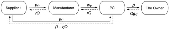
Figure 1.
The PCSC structure of single-supplier Stackelberg model.
It is realistic that many manufacturers have the monopoly on prefabricated components’ production technology, making them dominant in the PCSC. Therefore, in the Stackelberg model, we assume that the manufacturer acts as a leader, while the PC and supplier are followers. Profit functions of the PC, the manufacturer, and supplier 1 under the S model can be expressed as:
In Equation (1), the first term represents the revenue from selling prefabricated buildings; the second term represents the non-prefabricated materials from supplier 1 to the PC, and the third term represents the cost on purchasing prefabricated components from the manufacturer.
The first term includes the revenues of selling prefabricated components to the PC minus the costs of prefabricated raw materials and manufacturing. The second term means the investment of improving the prefabrication technology.
Equation (3) represents the revenue of selling all materials minus the production cost for supplier 1.
Optimal Decisions under S Structure
As followers in the S model, the PC and supplier 1 make decisions only after the manufacturer decides the optimal wholesale price. Therefore, optimal decisions in the decentralized model are solved using the Backward Induction Method, and we first find optimal reaction functions of followers, and then the optimal pricing decision of the leader is found. The optimal pricing decisions of three stakeholders are as follows:
Proposition 1.
.
Here, . The proof is provided in Appendix A.
In order to prove the existence of an optimal point in the function, the second partial derivative can be solved; if it is negative, the function has a maximum (optimal) value. This method has been widely used in similar pricing decision-making research for enterprises in the supply chain. In the S model, stakeholders’ profit functions are concave; therefore, optimal decisions exist. We get optimal pricing when the first partial derivative is equal to zero. Substituting optimal solutions into (1)–(3), members’ optimal profits are as follows:
As an important parameter, the prefabricated rate influences different stakeholders’ order volume and profits. Hence, we discuss the influence of the prefabricated rate on stakeholders’ decisions variables.
Proposition 2.
(1) ; ; if , when , ; if , when , , when , ; (2) ; ; .
The proof is provided in Appendix A.
From Proposition 2, firstly, the improvement in the prefabricated rate enhances the PC’s pricing decisions as order quantity increases with the prefabricated rate, which causes an increase in the sales price, so the marginal revenues for the PC are enhanced. Consequently, the supplier also enhances to obtain higher revenues. When the price sensitivity of the owner remains below a certain threshold and the prefabricated rate is low, the manufacturer curbs the rate to promote an increase in pricing due to reduced technical costs. Conversely, a high prefabricated level attracts the owner but also leads to a significant rise in technology costs; thus, the manufacturer improves the wholesale price to ensure profitability. Therefore, a high level of prefabricated rate is helpful to the manufacturer to achieve a higher pricing decision. Furthermore, it is intuitive that enhancing owner preferences contributes positively towards higher pricing decisions regardless of the prefabricated rate. It should be noted that if consumers exhibit a high price sensitivity and possess minimal preference for assembly, reducing the prefabricated rate would benefit the manufacturer more.
This discussion confirms that improving the prefabricated rate is beneficial to enhancing pricing decisions. As we can see from the above result, a high preference makes the price increase with the rising rate; thus, the government should strengthen the owner’s attention and requirements on the prefabricated rate.
The relationships between decision variables and the prefabricated rate are discussed. Consequently, we investigate the relationships between profits and the prefabricated rate.
Proposition 3.
(1) When , . (2) When , ; . (3) When , if , ; if , ; if , ; if or , .
Here, . The proof is provided in Appendix A.
Proposition 3 shows us that improving the prefabricated rate may not always yield increased revenues for all stakeholders. It is evident that the cost associated with prefabrication technology directly impacts manufacturers’ profits; thus, we recommend optimizing prefabrication techniques to minimize manufacturing costs. When the owner’s preference falls below a certain threshold, both the supplier’s and PC’s profits decrease proportionally. This can be attributed to an increase in production costs resulting from a higher prefabricated rate, prompting the leader to adjust pricing strategies for marginal revenues. However, the negative impact of price increases in orders that outweigh the positive effect of the rate increment, ultimately leading to the owner’s withdrawal. However, if the preference exceeds the threshold, profits initially increase but eventually decrease after r surpasses the threshold. Consequently, there exist optimal profit levels for both the supplier and PC. The rate increase leads to stakeholder profitability at a lower rate, but it becomes costly for stakeholders to remain profitable at a higher rate. Therefore, enterprises in the PCSC are advised to enhance consumers’ environmental awareness and preferences towards prefabricated buildings in order to stimulate an increase in order quantity with a corresponding rise in prefabricated rate. Nevertheless, it should be noted that an excessively high rate is not optimal for greater revenues.
3.2. Two-Supplier Stackelberg Model (T)
In practice, particularly during the construction phase, it is quite common for a PC to source prefabricated and non-prefabricated components from different suppliers due to the specialized nature of prefabrication manufacturing. This necessitates that each supplier meets specific qualification requirements and enters into separate contracts. Therefore, we will examine the case within a two-supplier framework.
Two suppliers are clear divisions of work. Supplier 1 only supplies the prefabricated raw materials to the manufacturer, while supplier 2 provides non-prefabricated raw materials for the PC directly. Similarly, the manufacturer produces and transfers prefabricated components to the PC. The PC assembles parts on the construction site and sells the finalized product to the owner. The T structure is shown in Figure 2.
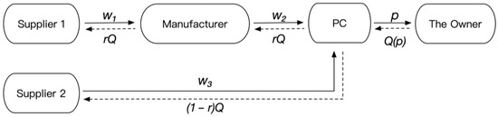
Figure 2.
The PCSC structure of two-supplier Stackelberg model.
When , the single-supplier structure could be a special case of the two-supplier structure. Similarly, in the Stackelberg model, the manufacturer acts as a leader, and the rest members are followers. The manufacturer takes the lead to make a decision on . Supplier 1 and supplier 2 make pricing decisions on and , respectively; then, the PC decides on the sale price p. All stakeholders are rational to maximize profits. Therefore, members’ profit functions can be expressed as:
The first term represents the revenue from selling prefabricated buildings; the second term represents the expenditure on non-prefabricated materials; the third term represents the payment to the manufacturer of prefabricated components.
Equation (9) represents the profit of supplier 1, which is equal to the revenue minus the production cost of prefabricated materials.
Equation (10) represents supplier 2’s revenues minus the cost of non-prefabricated materials.
The first term represents the sales revenue minus the costs of prefabricated raw materials and manufacturing, and the second term represents the investment on prefabrication technology.
Optimal Decisions under T Structure
In the Stackelberg model, the manufacturer still acts as a leader. All profit functions are concave, so optimal decisions of members can be expressed as follows.
Proposition 4.
,, , .
The proof is provided in Appendix A. Backward Induction Method. The solving process is similar to Proposition 1.
Profit functions are concave in the T structure. Therefore, an optimal decision exists for all stakeholders. Substitute them in Equations (8)–(11); the members’ optimal profits under the two-supplier structure are as follows:
From the results obtained under this model, we, surprisingly, find that supplier 1 and supplier 2 have the same optimal profits but different pricing decisions under the T structure.
As the important factor influencing pricing decisions, order quantity, and the degree of assembly, the prefabricated rate plays an essential role among stakeholders, so we next explore how the prefabricated rate affects decisions in under T structure.
Proposition 5.
, , , .
The proof is provided in Appendix A.
In Proposition 5, when the prefabricated rate rises, supplier 1 and the manufacturer should decrease their wholesale prices, while supplier 2 and the PC should increase their prices. This is because an increase in the prefabricated rate leads to a higher order quantity for the prefabricated channel, allowing for supplier 1 and the manufacturer to lower their prices accordingly. Conversely, due to a smaller order quantity, increasing ensures profitability for supplier 2. As a direct material supplier to the PC, an improvement in prompts the PC to raise its sale price in order to maintain marginal revenues.
The sensitivity analysis of decision variables in the T structure is examined above, and we now explore the sensitivity analysis between profits and the prefabricated rate in the following proposition.
Proposition 6.
(1) If , ; if , ; (2) If , ; if , , , .
The proof is provided in Appendix A.
From Proposition 6, the influence of the prefabricated rate on the followers’ profits is contingent upon their preference, while for the manufacturer, it depends on the cost coefficient. It is evident that as the cost of the prefabrication technology increases, the manufacturer experiences diminishing benefits with an increasing prefabricated rate. However, when the preference is over , indicating the active promotion of prefabricated construction by the government, owners tend to place larger orders with a higher prefabricated rate. Secondly, the profits of two suppliers increase with the prefabricated rate. It can be explained that the increases in the preference are more than the decline in price sensitivity in order quantity; then, suppliers and the PC benefit more from the increasing prefabricated rate. Conversely, if there is a weak preference for a higher prefabricated rate, the order quantity will decrease due to rising prices, causing owners to opt out of the PCSC, which causes loss in the profits of suppliers and the PC. For manufacturers, profits are directly linked to the cost of prefabrication technology. Therefore, it is imperative for governments to promote prefabricated construction and provide incentives aimed at improving owners’ preferences towards this mode of construction.
3.3. Dual-Channel Stackelberg Model with Two Suppliers (DT)
In practice, the supplier’s division of supply work is not clearly delineated. Therefore, we investigate how supplier 1 supplies prefabricated and non-prefabricated materials for the manufacturer or PC in this section. Considering the non-prefabricated order quantity as and the prefabricated materials order quantity as , we introduce an allocation proportion φ to represent the ratio of non-prefabricated materials’ supply besides the prefabricated materials , which is for supplier 1. Consequently, the remaining non-prefabricated materials are obtained from supplier 2, which accounts for a quantity of . The structural relationship of the DT structure is shown in Figure 3.
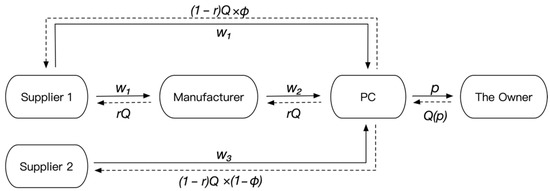
Figure 3.
The PCSC structure of two suppliers under the dual-channel Stackelberg model.
In the DT model, the manufacturer is still the leader in the prefabrication technology and decides the prefabricated components’ price (). Suppliers 1 and 2 submit their mission of supplying raw materials to the manufacturer or PC, and they have to make decisions after the leader’s decision. The stakeholders in the DT structure face the following profit function:
The first term of Equation (16) is the profit from selling assembled products; the second term represents the cost of purchasing part of the non-prefabricated materials from supplier 1, and the third term represents the cost of purchasing the remaining part, and the last term represents the cost of prefabricated components.
Equation (17) represents supplier 1’s revenues minus the production cost of the prefabricated materials and part of the non-prefabricated materials.
Equation (18) represents supplier 2’s revenues minus the cost of the rest of the non-prefabricated materials.
The first term represents the revenue minus the costs of procuring the prefabricated materials and manufacturing. The second term is the investment in prefabricated technology.
Optimal Decisions under DT Structure
In the dual-channel structure with two suppliers, the manufacturer is still the leader. The PC and two suppliers make decisions after the leader’s pricing decision. In this model, the optimal pricing decisions of different stakeholders are shown in proposition 7.
Proposition 7.
; ; ; .
The proof is provided in Appendix A.
Similarly, Backward Induction Method. We can get optimal decisions on pricing which we denote as . Therefore, ; then, substitute the optimal decisions and quantity into the profits function, obtaining the profits of the stakeholders are as follows:
Proposition 7 shows that stakeholders’ profit functions under the DT structure are concave, so there exist optimal decisions for all stakeholders. The prefabricated rate, as one of the important factors, greatly influences pricing decisions. Similarly, we discuss the influence of prefabricated rate on decisions.
Proposition 8.
(1) When , , ;
(2) when , ;
as , when , , when , , no restriction on ; when ,
(3) when , .
Where , , , .
The proof is provided in Appendix A.
Proposition 8 implies that suppliers, the PC, and the manufacturer’s decisions are closely correlated with the owner’s preference, price sensitivity, and supply allocation of non-prefabricated materials. If the owner pays low attention to the prefabricated rate, the two suppliers will cut wholesale prices to keep marginal revenues. Moreover, if only the owner’s preference exceeds a threshold, the two suppliers are motivated to improve wholesale prices, despite the price sensitivity being high. When the PC strengthens cooperation with supplier 1, φ is in , and the price sensitivity is above the threshold ; the threshold is positive, which means that the supplier’s pricing is influenced by the prefabricated rate preference. For the manufacturer, the preference directly influences sensitivity. When the preference exceeds , the wholesale price of the manufacturer increases with the prefabricated rate. Conversely, the manufacturer will decrease when the prefabricated rate increases.
In the DT structure, the order quantity is influenced by not only the prefabricated rate but also the allocation of non-prefabricated parts. The, above results also prove this, showing that the supply allocation has a great influence on members’ sensitivity to prefabricated rate. Therefore, we next explore the influence of the supply allocation φ on members’ decisions.
Proposition 9.
(1) ; (2) ; (3) If , ; when , ; (4) If , ; when , .
Where , , , . The proof is provided in Appendix A.
From Proposition 9, it is surprising that the wholesale of supplier 1 decreases with φ, despite supplier 1 having a larger share from the PC. This can be attributed to the fact that an increase in the order quantity renders supplier 1 more profitable. To foster collaboration with the PC, supplier 1 intends to reduce the wholesale price. Additionally, the manufacturer’s wholesale price also exhibits a decrease with φ. As the upstream enterprise, the manufacturer will decrease the wholesale price in response to supplier 1′s reduction in wholesale price. Although supplier 2 is compelled to divest a portion of the order quantity, when the owner’s preference for prefabricated construction is high, supplier 2 should augment to maximize marginal revenues. However, when the owner does not pay much attention to prefabricated rate, decreases with the proportion. Furthermore, as the owner’s preference for prefabricated buildings decreases, the PC’s pricing strategy experiences an increase in response to the growth of φ. This can be attributed to supplier 1 offering non-assembly parts at a higher wholesale price compared to supplier 2. As the PC strengthens its collaboration with supplier 1, the rise in prefabrication costs compels the PC to raise prices in order to offset the incurred loss.
In summary, when the PC strengthens partnerships with supplier 1, different stakeholders adopt distinct operational strategies for pricing decisions. The supplier 1 and the manufacturer reduce wholesale prices in response to increasing order quantities. For supplier 2, enhancing the owner’s attention to prefabricated rates and promoting environmental awareness are more advantageous for improving wholesale prices, while it is the contrary case for the PC.
4. Numerical Analysis
In this section, we present the numerical analysis to illustrate the theoretic results obtained above and the impact of prefabricated rate on operational decisions. We assume that . Similar numerical studies are widely used in the literature, such as Jiang and Yuan [45].
4.1. The Impact of Prefabricated Rate on Pricing Decisions in S and T Structures
According to Figure 4a, the sale price p and wholesale price increase with the prefabricated rate under the S structure, thus increasing the prefabricated rate is helpful for the PC and supplier to improve pricing decisions, while the wholesale price decreases firstly and then increases with the prefabricated rate, which is theoretical discussed in proposition 2; there is a threshold of prefabricated rate for the manufacturer. Therefore, only enhancing the prefabricated rate above a threshold will promote three stakeholders’ higher pricing. Furthermore, as the prefabricated rate approaches 1, the price increments of the supply chain members diminish in accordance with the economic principle of diminishing marginal benefits.
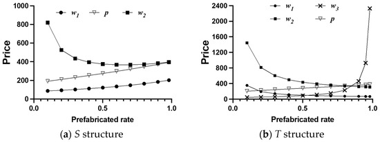
Figure 4.
Impact of prefabricated rate on members’ pricing decisions in S and T structures.
Figure 4b illustrates the sensitivity of prices and the prefabricated rate after the introduction of supplier 2. Similarly, the PC’s price increases with the prefabricated rate. However, when supplier 1 independently supplies prefabricated materials, the wholesale price decreases with the rate in the T structure, and does not experience an increase, which is different from the S structure. Supplier 2, responsible for non-prefabricated materials, will increase with the prefabricated rate. The same theoretical results are proven in proposition 5. When the rate approaches 1, supplier 2’s pricing experiences a significant surge due to the decrease in orders for non-prefabricated components. In order to prevent being excluded from the supply chain, supplier 2 resorts to substantially increasing its prices.
In the S and T structures, we find that the leader makes the highest pricing decision, but as the rate approaches an extremely high level in the T structure, supplier 2 performs the highest price. Moreover, within a moderate range of rates, both and exhibit greater values in the T structure. Therefore, in the T structure, it is not advisable to have extremely low or high levels of prefabricated rates due to significant differences in pricing decisions, which may result in reduced marginal revenues for certain stakeholders.
4.2. The Impact of Prefabricated Rate on Profits in S and T Structures
The relationships between stakeholders’ profits and the prefabricated rate are revealed in Figure 5a. Although the manufacturer assumes a dominant position in terms of pricing and market leadership, it does not necessarily yield the highest profits in the PCSC. Surprisingly, it is the supplier who reaps the greatest financial gains, while the PC’s profitability remains comparatively lower. Consequently, the PCSC with a single supplier deviates from conventional supply chains where the dominant entity retains higher profit margins. Furthermore, the profits of the PC decline with the prefabricated rate, while both the manufacturer and supplier identify their optimal rates to maximize profitability. Notably, the supplier’s optimal prefabricated rate surpasses that of the manufacturer. As r approaches 1, profit reductions occur more rapidly, indicating that excessively high levels of prefabrication are not advantageous in the S structure. Rather, a moderate rate is deemed feasible for the PCSC with an S structure.
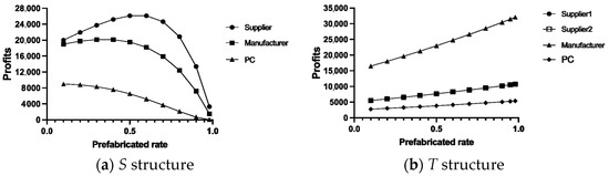
Figure 5.
Impact of prefabricated rate on members’ profits in S and T structures.
After incorporating supplier 2 into the PCSC, Figure 5b reveals the correlation between stakeholders’ profits and the prefabricated rate. Both suppliers exhibit similar profit trends, with the manufacturer attaining the highest profits, while the PC’s profits remain comparatively lower. Additionally, all stakeholders experience increasing profits as the prefabricated rate rises, confirming Proposition 6. Therefore, the T structure is more conducive to the long-term stable development of the prefabricated construction industry in practice. We recommend that the manufacturer enhances the prefabricated rate to benefit the PCSC in the T structure.
4.3. The Impact of Prefabricated Rate and Supply Allocation in DT Structure
In Figure 6a, when is at a low level (supplier 1 has a low collaboration with the PC), the pricing decisions of two suppliers and the manufacturer decrease with the prefabricated rate, while only the PC’s increases. However, in Figure 6b,c, there is a transition in sensitivity for the price changes of both suppliers from a decrease to an increase. Therefore, exists a threshold that makes the wholesale price of the two suppliers change with the trend of increasing prefabricated rate. Moreover, as goes up, supplier 1’s, the manufacturer’s, and the PC’s price drops, while supplier 2’s price increases, which meets the conclusion of Proposition 9.
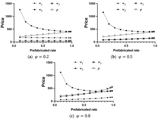
Figure 6.
Impact of prefabricated rate and supply allocation on pricing decisions in DT structure.
With a higher , the pricing decisions of the PC exhibit minimal fluctuations. Despite the strengthened collaboration with supplier 1, particularly in terms of supply allocation, the PC’s pricing remains relatively stable. We can explain that even when undergoes changes, the non-prefabricated and prefabricated materials for the PC remain unchanged, resulting in negligible impact on its pricing.
Profits curve under the DT structure are presented in Figure 7: the PC’s and supplier 2’s decrease with the prefabricated rate, and supplier 1’s profits are concave, which can derive an optimal prefabricated rate. Moreover, the extreme point moves towards the upper right direction with φ, implying a greater optimal profit and rate. From the manufacturer, there is an overall downward trend in profits. With increasing φ, the manufacturer’s profit curve is more concave; thus, the optimal profits are greater. Also, for the supplier, the magnitude of the profit change increases with the prefabricated rate, and the extreme point gets greater. Thus, enhancing the supply allocation is beneficial to obtain greater optimal profits. However, when the rate approaches 1, the decline in the members’ profits gets faster, implying the fact that enhancing the prefabricated rate to an extremely high level is not beneficial for all stakeholders in the DT structure. Instead, a moderate rate is advisable. Moreover, there are optimal prefabricated rates for supplier 1 and the manufacturer, which provides practical guides for enterprises to maximize profits through deciding a proper rate in the PCSC.
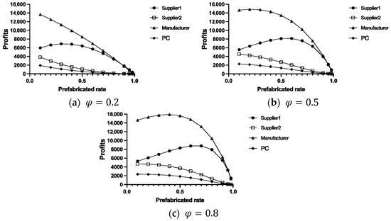
Figure 7.
Impact of prefabricated rate and supply allocation on profits in DT structure.
4.4. Comparative Analysis among the Three Models
In the S structure, supplier 1 is responsible for the whole supply work, including prefabricated and non-prefabricated parts; thus, in the T and DT structures, we regard supplier 1 and supplier 2 as a whole entity. We denote the supplier’s profits under the T and DT structures as and , respectively. In the DT model, we select the highest profit level (when ) to compare with the other two models.
Figure 8 compares the profit levels of the PC, manufacturer, and supplier under the three structures, respectively. The intersection point of profit between the S and T structures always exists. When the prefabricated rate exceeds this intersection point, the profit of each member in the T structure will surpass that of the S structure. It is evident that the profits of all supply chain members are generally lower in the DT structure () compared to the other two structures, except for supplier 1. Specifically, we analyze the profit difference between supplier 1 and supplier 2 in both the T and DT structures, as depicted in Figure 9. The selection of channels between the T and DT structures is available for supplier 1. Supplier 1 opts for the DT structure instead of the T structure only when it achieves a moderate prefabricated rate, indicating its higher inclination to collaborate with the PC. This preference arises due to the reinforcement of the order share for supplier 1 within the DT structure, leading to increased profitability. However, supplier 1 incurs higher production costs compared to supplier 2, resulting in a decrease in both the marginal revenue and profit for the manufacturer and PC. Additionally, as the order decreases, there is also a decline in revenue for supplier 2.
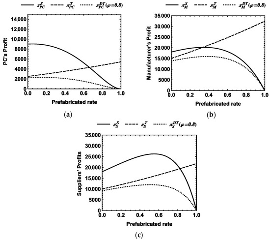
Figure 8.
Impact of prefabricated rate on supply chain members’ profit among the three structures.
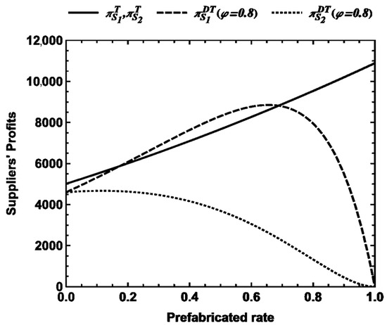
Figure 9.
Impact of prefabricated rate on suppliers’ profit in T and DT structures.
Figure 10 shows the profit curves for the three structural supply chains. It is visually evident from the figures that the profit curve of the DT model consistently remains at its lowest point, indicating a lower income generation. Therefore, it is advisable to avoid forming a DT structure by carefully considering the relationship among each member. If a DT structure is formed due to inter-member relationships, an increase in supplier 1’s sharing rate should be considered. Furthermore, the profit curves of the S and T models intersect at a specific point. When below this intersection, it is recommended to promote a supply chain with a single supplier contracting all raw materials. On the other hand, when above this intersection point, it is suggested to have two suppliers independently contracted for prefabricated and non-prefabricated materials. Currently, the lowest prefabricated rate in China is concentrated in 50% of all provinces, so the S structure is more applicable.
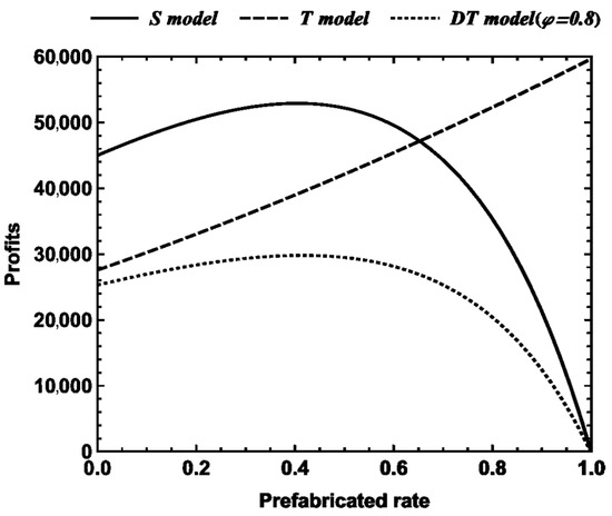
Figure 10.
Impact of prefabricated rate on supply chain profits among the three structures.
5. Conclusions and Future Research Directions
This paper examines a manufacturer-dominated PCSC consisting of suppliers, a manufacturer, and a PC, and considers the impact of consumer preferences for the prefabricated rate on the market demand and the diversion effect of the prefabricated rate on the supply chain. Additionally, we explore pricing decisions within three structural models (S, T, and DT models). The proposed model analytically and numerically illustrates some key channel strategies for choosing the structures for stakeholders. The main results and managerial insights are as follows:
- (1)
- Under the S structure, the PCSC is with a single supplier. The only supplier shoulders both the prefabricated and non-prefabricated materials. All stakeholders have optimal pricing decisions and profits. Moreover, the owner’s preference greatly influences the sensitivity of profits; thus, an effective approach is to showcase the eco-friendly attributes of prefabricated buildings to consumers. If the PCSC adopts an S-structure model, a moderate prefabricated rate is advisable instead of a high level of rate. Currently, the lowest prefabricated rate in China is concentrated in 50% of all provinces; thus, indicating a higher applicability of the S structure.
- (2)
- When two suppliers respectively shoulder the prefabricated and non-prefabricated materials’ supply, the T structure is formed. Firstly, improving the prefabricated rate is beneficial to the PC and supplier 2 but detrimental to supplier 1 and the manufacturer in enhancing pricing decisions. However, followers’ profits are related to the preference of the owner to the prefabricated rate; when the owner pays great attention to the prefabricated rate because of the consuming market or government’s policies, the prefabricated rate’s enhancement is profitable to followers. As for the leader, the manufacturer’s profits are associated with the investment in prefabrication technology. Improving independent research and technical efficiency are suggested to improve the consumers’ satisfaction and members’ revenues. If the PCSC adopts a T-structure model, enterprises should avoid extremely low or high prefabricated rates due to the significant difference in pricing decision. However, from an enterprise profit perspective, increasing the prefabricated rate leads to higher profits for all stakeholders in the supply chain. Therefore, the T structure is more conducive to the long-term stable development of the prefabricated construction industry in practice.
- (3)
- When there are no longer independent divisions of supply, supplier 1 will shoulder some of the non-prefabricated materials besides prefabricated materials, while the other has less close cooperation and shoulders the rest non-prefabricated materials. In the DT structure, the dominant manufacturer gains the greatest profits. If the PC has a close supplier, allocating a larger proportion of non-prefabricated parts to supplier1 would yield higher profitability for stakeholders involved in prefabrication. Moreover, though the high prefabricated rate improves pricing for most members except the manufacturer, it hurts members’ revenues. Therefore, it is advisable to maintain a moderate prefabricated rate.
From the stakeholders’ perspective, in terms of channel selection, it is recommended to carefully consider the relationship between each member and avoid forming the DT structure since it yields lower profits for supply chain members (PC, manufacturer, and supplier 2) compared to the S structure and T structure. If a DT structure is formed due to members’ relationships, the PC should consider strengthening cooperation with supplier 1 to enhance profitability for all parties involved. Changes in material supply structures have minimal impact on the PC’s pricing as both prefabricated and non-prefabricated materials remain consistent regardless of the supply structure. When the prefabricated rate is moderate, supplier 1 will opt for the DT structure instead of the T structure. In order to ensure the highest profit in the supply chain, the manufacturer should choose the T structure or the DT structure as two supply modes.
This study has several limitations and opportunities for a future extension. Firstly, the model in our study considers one prefabricated company, one manufacturer, and two suppliers; however, it is more realistic to include multiple manufacturers throughout the entire life cycle of prefabricated buildings. Secondly, the government plays a crucial role in implementing prefabricated buildings; thus, we should consider the government’s intervention measures [35,57]. Finally, carbon emissions occur during the production and prefabrication process of prefabricated buildings; henceforth, studying the influence of carbon policies on the prefabricated building supply chain would be valuable.
Author Contributions
Conceptualization, W.J. (Wen Jiang), M.Y. and Y.H.; Formal analysis, Y.H. and M.Y.; Project administration, W.J. (Wen Jiang) and W.J. (Weiling Jiang); Writing—original draft, Y.H. and M.Y.; Supervision, W.J. (Wen Jiang), W.J. (Weiling Jiang) and I.M.; Writing—review and editing, Y.H. and I.M. All authors have read and agreed to the published version of the manuscript.
Funding
This work was funded by National Natural Science Foundation of China (No.71972136) and Sichuan Science and Technology Program (No. 2022JDTD0022).
Institutional Review Board Statement
Not applicable.
Informed Consent Statement
Not applicable.
Data Availability Statement
Data are contained within the article.
Conflicts of Interest
The authors declare no conflicts of interest.
Abbreviations
| PCSC | Prefabricated Construction Supply Chain |
| CEA | Consumer Environmental Awareness |
Appendix A
Proof of Proposition 1.
As a follower, the PC has to make decisions only after the leader’s (manufacturer’s) decisions, which means in the backward induction, we should first solve the followers’ optimal reaction function. Because , implying that the optimal decision of exits, and PC’s optimal reaction function can be solved when , which is ; then, . At the same time, we should solve the optimal reaction function because of the dual-channel structure. Similar to the PC’s solving process, we have , so the optimal decision can be found when , which is . As the leader, the manufacturer has superior power that makes a decision after observing the followers’ decisions. In other words, the manufacturer will find the optimal pricing decision based on the reaction functions of the PC and supplier. Substituting and into (2), we have the profit function . Because , we can find an optimal when , which is . Simultaneously solving and , we will get optimal pricing decisions under the dual-channel structure with a single supplier, which are as follows: , . Then, substitute and into : □
Proof of Proposition 2.
In the single-supplier structure,
and . To ensure that the PC’s profit is positive, we have ; then, . Firstly, . It is easy to get that . Secondly, ; when it is equal to 0, we have and . If , , ; when , . If , , ; when , ; when , . When , if , there is no restriction on , but if , has to satisfy . Thirdly, , as we get ; then, . Thus, . Fourthly, it is easy to prove ; ; . □
Proof of Proposition 3.
. If . ; has solutions, and . We have ; then, . The positive/negative judgments of and the range of are displayed in Table A1.
Table A1.
The positive/negative judgments of and the range of .
Table A1.
The positive/negative judgments of and the range of .
| \ | \ | \ | ||||
. Under the assumption, there are solutions when , and , , ; therefore, the positive/negative judgments of and the range of are displayed in Table A2.
Table A2.
The positive/negative judgments of and the range of .
Table A2.
The positive/negative judgments of and the range of .
| \ | \ | \ | |||
; ; . □
Proof of Proposition 4.
First, the profit of PC is a concave function in
because ; then, , and there is an optimal reaction, which is . As , we can substitute in the ; then, , so we have . Secondly, we have two suppliers’ second derivative respectively. , . Both suppliers have optimal reaction functions when the first partial derivatives satisfy and , so . Next, we solve simultaneous equations, which are . Bringing the two decisions into , and Equation (11), we find ; thus, the optimal margin profit for the manufacturer has , so . Substituting in the optimal decisions, we can get decisions under the two-supplier structure: ,, , . □
Proof of Proposition 5.
, , , . □
Proof of Proposition 6.
, , . As , for positive revenues of stakeholders, we have premises that , , , so . , , and have the same molecule, and the denominators are greater than 0; then, we only analyze . Therefore, when , ; then, , ; when , , . Similarly, when , ; when , . □
Proof of Proposition 7.
First of all, according to Equation (12), , is a concave function about , so there is an optimal solution. When , the optimal reaction function is . Bringing it back to , as (13) and (14), we find the second partial derivatives , . Hence, supplier 1 and supplier 2 have concave functions of decision variables, where the optimal reaction functions are and . Consequently, and are simultaneously solved, so ,. Bring into ; then, based on Equation (15), we get the second derivative of . When , . Then, optimal decisions including can be expressed as: ; ; . □
Proof of Proposition 8.
According to the DT structure and assumptions, we have .
; . and have similar expressions; therefore, the sensitivity is the same. When , ; when , ; as , when , ; when , . There is no restriction on ; when , . , as the denominator of the fraction is positive, we only judge the numerator. We assume ; then, , . Similarly, we only discuss the numerator. We assume . Then, . □
Proof of Proposition 9.
. It is easy to prove and . ; as the denominator of the fraction is positive, we only judge the numerator. If , the numerator is negative; then, ; if , . As , . Likewise, . If , the numerator is positive; then, ; if , . As , . □
References
- Zhai, Y.; Zhong, R.Y.; Huang, G.Q. Towards Operational Hedging for Logistics Uncertainty Management in Prefabrication Construction. IFAC-Pap. 2015, 48, 1128–1133. [Google Scholar] [CrossRef]
- Tam, V.W.Y.; Tam, C.M.; Chan, J.K.W.; Ng, W.C.Y. Cutting Construction Wastes by Prefabrication. Int. J. Constr. Manag. 2006, 6, 15–25. [Google Scholar] [CrossRef]
- Shen, K.; Cheng, C.; Li, X.; Zhang, Z. Environmental Cost-Benefit Analysis of Prefabricated Public Housing in Beijing. Sustainability 2019, 11, 207. [Google Scholar] [CrossRef]
- Aye, L.; Ngo, T.; Crawford, R.H.; Gammampila, R.; Mendis, P. Life Cycle Greenhouse Gas Emissions and Energy Analysis of Prefabricated Reusable Building Modules. Energy Build. 2012, 47, 159–168. [Google Scholar] [CrossRef]
- Navaratnam, S.; Ngo, T.; Gunawardena, T.; Henderson, D. Performance Review of Prefabricated Building Systems and Future Research in Australia. Buildings 2019, 9, 38. [Google Scholar] [CrossRef]
- Ministry of Housing and Urban-Rural Development of the People’s Republic of China (MOHURD). 2017; Standard for as-Sessment of Prefabricated Building. Available online: https://www.mohurd.gov.cn/xinwen/gzdt/201801/20180124_234930.html (accessed on 1 January 2024).
- Criscuolo, C.; Martin, R.; Overman, H.G.; Van Reenen, J. Some Causal Effects of an Industrial Policy. Am. Econ. Rev. 2019, 109, 48–85. [Google Scholar] [CrossRef]
- Chitra, K. In Search of the Green Consumers: A Perceptual Study. J. Serv. Res. 2007, 7, 173. [Google Scholar]
- Zhou, Z.; Shen, G.; Xue, J.; Sun, C.; Liu, Y.; Cong, W.; Yu, T.; Wang, Y. The Formation of Citizens’ Intentions to Purchase Prefabricated Housing in China: The Integrating Theory of Planned Behavior and Norm Activation Model. Eng. Constr. Archit. Manag. 2023. ahead-of-print. [Google Scholar] [CrossRef]
- Zhou, J.; Li, Y.; Ren, D. Quantitative Study on External Benefits of Prefabricated Buildings: From Perspectives of Economy, Environment, and Society. Sustain. Cities Soc. 2022, 86, 104132. [Google Scholar] [CrossRef]
- GOSC. General Office of the CPC Central Committee, General Office of the State Council (2021). Opinions on Promoting Green Development of Urban and Rural Construction. Available online: https://www.gov.cn/zhengce/2021-10/21/content_5644083.htm (accessed on 1 January 2024).
- Jaillon, L.; Poon, C.S. Sustainable Construction Aspects of Using Prefabrication in Dense Urban Environment: A Hong Kong Case Study. Constr. Manag. Econ. 2008, 26, 953–966. [Google Scholar] [CrossRef]
- Xu, Z.; Zayed, T.; Niu, Y. Comparative Analysis of Modular Construction Practices in Mainland China, Hong Kong and Singapore. J. Clean. Prod. 2020, 245, 118861. [Google Scholar] [CrossRef]
- GB/T 51129-2017; Standard for Assessment of Prefabricated Building. Ministry of Housing and Urban-Rural Development of the People’s Republic of China (MOHURD): Beijing, China, 2017. (In Chinese)
- Xu, A.; Zhu, Y.; Wang, Z.; Zhao, Y. Carbon Emission Calculation of Prefabricated Concrete Composite Slabs during the Production and Construction Stages. J. Build. Eng. 2023, 80, 107936. [Google Scholar] [CrossRef]
- Du, Q.; Bao, T.; Li, Y.; Huang, Y.; Shao, L. Impact of Prefabrication Technology on the Cradle-to-Site CO2 Emissions of Residential Buildings. Clean Technol. Environ. Policy 2019, 21, 1499–1514. [Google Scholar] [CrossRef]
- Hong, J.; Shen, G.Q.; Li, Z.; Zhang, B.; Zhang, W. Barriers to Promoting Prefabricated Construction in China: A Cost–Benefit Analysis. J. Clean. Prod. 2018, 172, 649–660. [Google Scholar] [CrossRef]
- Balderjahn, I. Personality Variables and Environmental Attitudes as Predictors of Ecologically Responsible Consumption Patterns. J. Bus. Res. 1988, 17, 51–56. [Google Scholar] [CrossRef]
- Hong, Z.; Guo, X. Green Product Supply Chain Contracts Considering Environmental Responsibilities. Omega 2019, 83, 155–166. [Google Scholar] [CrossRef]
- Wang, Y.; Hou, G. A Duopoly Game with Heterogeneous Green Supply Chains in Optimal Price and Market Stability with Consumer Green Preference. J. Clean. Prod. 2020, 255, 120161. [Google Scholar] [CrossRef]
- Liu, Z.L.; Anderson, T.D.; Cruz, J.M. Consumer Environmental Awareness and Competition in Two-Stage Supply Chains. Eur. J. Oper. Res. 2012, 218, 602–613. [Google Scholar] [CrossRef]
- Zhang, L.; Wang, J.; You, J. Consumer Environmental Awareness and Channel Coordination with Two Substitutable Products. Eur. J. Oper. Res. 2015, 241, 63–73. [Google Scholar] [CrossRef]
- Zhou, H.; Duan, Y. Online Channel Structures for Green Products with Reference Greenness Effect and Consumer Environmental Awareness (CEA). Comput. Ind. Eng. 2022, 170, 108350. [Google Scholar] [CrossRef]
- Long, Q.; Tao, X.; Shi, Y.; Zhang, S. Evolutionary Game Analysis Among Three Green-Sensitive Parties in Green Supply Chains. IEEE Trans. Evol. Comput. 2021, 25, 508–523. [Google Scholar] [CrossRef]
- Chen, S.; Su, J.; Wu, Y.; Zhou, F. Optimal Production and Subsidy Rate Considering Dynamic Consumer Green Perception under Different Government Subsidy Orientations. Comput. Ind. Eng. 2022, 168, 108073. [Google Scholar] [CrossRef]
- Liu, M.; Li, Z.; Anwar, S.; Zhang, Y. Supply Chain Carbon Emission Reductions and Coordination When Consumers Have a Strong Preference for Low-Carbon Products. Environ. Sci. Pollut. Res. 2021, 28, 19969–19983. [Google Scholar] [CrossRef] [PubMed]
- Zhang, W.; He, L.; Yuan, H. Enterprises’ Decisions on Adopting Low-Carbon Technology by Considering Consumer Perception Disparity. Technovation 2022, 117, 102238. [Google Scholar] [CrossRef]
- Liang, L.; Futou, L. Differential Game Modelling of Joint Carbon Reduction Strategy and Contract Coordination Based on Low-Carbon Reference of Consumers. J. Clean. Prod. 2020, 277, 123798. [Google Scholar] [CrossRef]
- Wen, D.; Xiao, T.; Dastani, M. Pricing and Collection Rate Decisions in a Closed-Loop Supply Chain Considering Consumers’ Environmental Responsibility. J. Clean. Prod. 2020, 262, 121272. [Google Scholar] [CrossRef]
- Zhang, S.; Wang, C.; Yu, C.; Ren, Y. Governmental Cap Regulation and Manufacturer’s Low Carbon Strategy in a Supply Chain with Different Power Structures. Comput. Ind. Eng. 2019, 134, 27–36. [Google Scholar] [CrossRef]
- Xia, L.; Hao, W.; Qin, J.; Ji, F.; Yue, X. Carbon Emission Reduction and Promotion Policies Considering Social Preferences and Consumers’ Low-Carbon Awareness in the Cap-and-Trade System. J. Clean. Prod. 2018, 195, 1105–1124. [Google Scholar] [CrossRef]
- Tong, W.; Mu, D.; Zhao, F.; Mendis, G.P.; Sutherland, J.W. The Impact of Cap-and-Trade Mechanism and Consumers’ Environmental Preferences on a Retailer-Led Supply Chain. Resour. Conserv. Recycl. 2019, 142, 88–100. [Google Scholar] [CrossRef]
- Xu, C.; Jing, Y.; Shen, B.; Zhou, Y.; Zhao, Q.Q. Cost-Sharing Contract Design between Manufacturer and Dealership Considering the Customer Low-Carbon Preferences. Expert Syst. Appl. 2023, 213, 118877. [Google Scholar] [CrossRef]
- Liu, S.; Li, Z.; Teng, Y.; Dai, L. A Dynamic Simulation Study on the Sustainability of Prefabricated Buildings. Sustain. Cities Soc. 2022, 77, 103551. [Google Scholar] [CrossRef]
- He, L.; Chen, L. The Incentive Effects of Different Government Subsidy Policies on Green Buildings. Renew. Sustain. Energy Rev. 2021, 135, 110123. [Google Scholar] [CrossRef]
- Fan, K.; Wu, Z. Incentive Mechanism Design for Promoting High-Level Green Buildings. Build. Environ. 2020, 184, 107230. [Google Scholar] [CrossRef]
- Jiang, L.; Li, Z.; Li, L.; Gao, Y. Constraints on the Promotion of Prefabricated Construction in China. Sustainability 2018, 10, 2516. [Google Scholar] [CrossRef]
- Wang, Z.; Hu, H.; Gong, J.; Ma, X.; Xiong, W. Precast Supply Chain Management in Off-Site Construction: A Critical Literature Review. J. Clean. Prod. 2019, 232, 1204–1217. [Google Scholar] [CrossRef]
- Ma, Z.; Yang, Z.; Liu, S.; Wu, S. Optimized Rescheduling of Multiple Production Lines for Flowshop Production of Reinforced Precast Concrete Components. Autom. Constr. 2018, 95, 86–97. [Google Scholar] [CrossRef]
- Wang, Z.; Hu, H. Improved Precast Production–Scheduling Model Considering the Whole Supply Chain. J. Comput. Civ. Eng. 2017, 31, 04017013. [Google Scholar] [CrossRef]
- Zhai, Y.; Zhong, R.Y.; Li, Z.; Huang, G. Production Lead-Time Hedging and Coordination in Prefabricated Construction Supply Chain Management. Int. J. Prod. Res. 2017, 55, 3984–4002. [Google Scholar] [CrossRef]
- Zhai, Y.; Zhong, R.Y.; Huang, G.Q. Buffer Space Hedging and Coordination in Prefabricated Construction Supply Chain Management. Int. J. Prod. Econ. 2018, 200, 192–206. [Google Scholar] [CrossRef]
- Zhai, Y.; Fu, Y.; Xu, G.; Huang, G. Multi-Period Hedging and Coordination in a Prefabricated Construction Supply Chain. Int. J. Prod. Res. 2019, 57, 1949–1971. [Google Scholar] [CrossRef]
- Han, Y.; Skibniewski, M.J.; Wang, L. A Market Equilibrium Supply Chain Model for Supporting Self-Manufacturing or Outsourcing Decisions in Prefabricated Construction. Sustainability 2017, 9, 2069. [Google Scholar] [CrossRef]
- Jiang, W.; Yuan, M. Coordination of Prefabricated Construction Supply Chain under Cap-and-Trade Policy Considering Consumer Environmental Awareness. Sustainability 2022, 14, 5724. [Google Scholar] [CrossRef]
- Isatto, E.L.; Azambuja, M.; Formoso, C.T. The Role of Commitments in the Management of Construction Make-to-Order Supply Chains. J. Manag. Eng. 2015, 31, 04014053. [Google Scholar] [CrossRef]
- Jiang, W.; Qi, X. Pricing and Assembly Rate Decisions for a Prefabricated Construction Supply Chain under Subsidy Policies. PLoS ONE 2022, 17, e0261896. [Google Scholar] [CrossRef] [PubMed]
- Du, Q.; Hao, T.; Huang, Y.; Yan, Y. Prefabrication Decisions of the Construction Supply Chain under Government Subsidies. Environ. Sci. Pollut. Res. 2022, 29, 59127–59144. [Google Scholar] [CrossRef] [PubMed]
- Han, Y.; Wang, L.; Kang, R. Influence of Consumer Preference and Government Subsidy on Prefabricated Building Developer’s Decision-Making: A Three-Stage Game Model. J. Civ. Eng. Manag. 2023, 29, 35–49. [Google Scholar] [CrossRef]
- Wang, D.-Y.; Wang, X. Supply Chain Consequences of Government Subsidies for Promoting Prefabricated Construction and Emissions Abatement. J. Manag. Eng. 2023, 39, 04023029. [Google Scholar] [CrossRef]
- Jayawardana, J.; Sandanayake, M.; Jayasinghe, J.A.S.C.; Kulatunga, A.K.; Zhang, G. A Comparative Life Cycle Assessment of Prefabricated and Traditional Construction—A Case of a Developing Country. J. Build. Eng. 2023, 72, 106550. [Google Scholar] [CrossRef]
- Li, Y.; Tong, Y.; Ye, F.; Song, J. The Choice of the Government Green Subsidy Scheme: Innovation Subsidy vs. Product Subsidy. Int. J. Prod. Res. 2020, 58, 4932–4946. [Google Scholar] [CrossRef]
- Qian, Y.; Yu, X.; Shen, Z.; Song, M. Complexity Analysis and Control of Game Behavior of Subjects in Green Building Materials Supply Chain Considering Technology Subsidies. Expert Syst. Appl. 2023, 214, 119052. [Google Scholar] [CrossRef]
- Ji, Y.; Qi, K.; Qi, Y.; Li, Y.; Li, H.X.; Lei, Z.; Liu, Y. BIM-Based Life-Cycle Environmental Assessment of Prefabricated Buildings. Eng. Constr. Archit. Manag. 2020, 27, 1703–1725. [Google Scholar] [CrossRef]
- Ministry of Housing and Urban-Rural Development of the People’s Republic of China (MOHURD). 2019; Standard for Quality Management of Precast Concrete Member Fabricated in the Plant. Available online: https://www.mohurd.gov.cn/gongkai/zhengce/zhengcefilelib/201904/20190422_240274.html (accessed on 1 January 2024).
- Qi, L.; Shi, J.; Xu, X. Supplier Competition and Its Impact on Firm’s Sourcing Strategy. Omega 2015, 55, 91–110. [Google Scholar] [CrossRef]
- Xie, L.; Liu, Y.; Han, H.; Qiu, C.M. Outsourcing or Reshoring? A Manufacturer’s Sourcing Strategy in the Presence of Government Subsidy. Eur. J. Oper. Res. 2023, 308, 131–149. [Google Scholar] [CrossRef]
Disclaimer/Publisher’s Note: The statements, opinions and data contained in all publications are solely those of the individual author(s) and contributor(s) and not of MDPI and/or the editor(s). MDPI and/or the editor(s) disclaim responsibility for any injury to people or property resulting from any ideas, methods, instructions or products referred to in the content. |
© 2024 by the authors. Licensee MDPI, Basel, Switzerland. This article is an open access article distributed under the terms and conditions of the Creative Commons Attribution (CC BY) license (https://creativecommons.org/licenses/by/4.0/).