Pricing Problems in the Pharmaceutical Supply Chain with Mixed Channel: A Power Perspective

Abstract

This paper builds Pharmaceutical Manufacturer Stackelberg, Pharmacy Stackelberg and Nash game models with and without price cap regulation. The optimal pricing, performance and social welfare are derived and compared in three different power structures to find out how price cap regulation and power structures affect the drug supply chain. More power over other supply chain members always allows the pharmaceutical manufacturer to obtain more profits. However, the pharmacy cannot always benefit from its dominant position in the market with changes in the wholesale price cap. Additionally, the balanced market structure may harm social welfare under certain conditions. Another interesting finding is that the restricted wholesale price cap deeply affects the financial performance and social welfare in the manufacturer-dominated and pharmacy-dominated markets. The research results can provide important management insights, which will be beneficial to the government to design smart price-limiting policies that take into account the power relationships of the supply chain.

1. Introduction

There has been growth in the global drug industry in recent years, which the whole world valued at about $1.2 trillion in 2018 [1]. As a special product, the high price of medicines has been a high concern of the governments, insurers and patients. Since the 21st century, China’s per capita medical and health expenditure for urban and rural residents has grown rapidly, from 171.09 yuan in 2000 to 1479.28 yuan in 2018. Expensive medical expenditure may cause many social problems and even threaten the financial sustainability of public health systems [2]. Governments in both developing and developed countries have enacted measures to restrict medical institutions from overcharging patients [3,4,5,6]. Price cap regulation and external reference pricing are the two most commonly used drug price control mechanisms for reducing the burden of patients in most countries around the world [7,8].

In China, price cap regulation and “expensive medical treatment” policy are applied to address the serious social problem of “expensive medical care”. However, setting maximum prices for drugs may cause pharmaceutical companies to exit the market and increase the risk of drug shortages [3,9,10]. Patients may pay higher fees for imported drugs with the same curative effect [11,12]. Thus, policymakers should consider both social and economic benefits in order to ensure the successful implementation of policies.

However, different power structures have a significant impact on the profit of a single company and the profitability of the whole supply chain. In real life, power structure also exists in drug supply chain. The role of drug manufacturers is particularly important for anticancer drugs that require a long development period—in addition, selling day-to-day care drugs or services such as obesity, with independent or chain pharmacies leading the way.

Reasonable pricing of medicines is crucial to the social welfare of the people. Welfare economics considers welfare to be divided into three dimensions: individual, social and economic. Social welfare usually refers to the collection of the whole welfare obtained by a certain social group for more people. Taking China as an example, despite the increasing income level of the people, the high cost of drugs is still unaffordable for most ordinary people, which makes the people complain. Bargaining power in the market largely affects the profits that enterprises can obtain. Chen et al. and Danzon et al. discussed the impact of various price cap regulations on the pricing, profits, and social welfare of the pharmaceutical supply chain when the pharmaceutical manufacturer is Stackelberg leader [3,13]. Zheng et al. established four price cap models for the offline-to-online pharmaceutical supply chain when the pharmacy dominates in the market [2]. Previous studies focused on the important role of different price cap regulations while ignoring the effects of the power structure on the pharmaceutical supply chain. In this paper, power structures and price cap regulation are considered to investigate the pharmaceutical supply chain. Some key questions will be discussed.

(1)

What effects do power structures have on pricing, performance and social welfare in the pharmaceutical supply chain where the pharmaceutical manufacturer is regulated?

(2)

How does the restricted wholesale price cap affect the financial performance and social welfare in three different power structures?

This paper focuses on a two-echelon supply chain including a pharmaceutical manufacturer and a pharmacy with an O2O mixed channel. The government imposes price caps on the pharmaceutical manufacturer. We establish three basic models and price cap regulation models (including Pharmaceutical Manufacturer Stackelberg, Pharmacy Stackelberg, Vertical Nash) respectively. The optional pricing, profits and social welfare in three different power structures are obtained through game theory. By comparing the model equilibriums in the above models and performing sensitivity analysis on the restricted price cap (θ), we find out how power structures and wholesale price cap affect economic and social performance.

The main contributions of this paper are as follows: (i) it complements the existing studies on price in the pharmaceutical supply chain through a comprehensive examination of the effects of price cap and supply chain power relationships on pharmaceutical firms’ which are in mixed channel operational decisions and the consequential economic and social performance of the supply chain. It provides a foundation for exploring the cross-effects of other price cap regulations (pharmacy price cap regulation and linkage price cap regulation) and power structures on the pharmaceutical supply chain. (ii) Our research provides insights for policymakers to take a novel approach for evaluating regulatory policies on price standards of pharmaceutical products by modeling the decision of the pharmaceutical firms and the associated economic and social performance of the supply chain. Such an approach enables regulators to develop appropriate price regulations to improve the sustainability of the pharmaceutical supply chain, thereby safeguarding social welfare and pharmaceutical firms’ profitability. (iii) Insights derived from the analytical results provide important managerial implications that support pharmaceutical firms in making operational decisions to sustain market competitiveness.

The rest of the paper is organized as follows. Section 2 presents a brief review of the relevant literature. Section 3 presents model descriptions and assumptions. Section 4 presents mathematical models and equilibrium analysis. In Section 5, we discuss the effects of power structures on the pharmaceutical supply chain. In Section 6, we discuss the effects of the price cap regulation on the pharmaceutical supply chain. Section 7 summarizes the important findings of the paper and points out the limitations of mathematical models and future research directions.

2. Literature

This paper reviews three streams of literature that are particularly relevant: (i) price cap regulations in the pharmaceutical supply chain; (ii) power structure in the supply chain; (iii) social welfare in the supply chain.

Price cap regulation in pharmaceutical supply chain 

 

Governments in most countries set maximum selling prices for medicines to prevent medical firms from charging patients excessively. Abbott III found that at first, the price cap in a regulated market is higher than the price in an unregulated market, and the price in an unregulated market would exceed that in a regulated market in few years [14]. Zheng et al. proposed that linkage price cap regulation can improve both financial performance and social welfare [2]. However, some studies show that price cap regulation may bring unexpected results. Price cap regulations discourage market competition including brand-name drugs and generic drugs [13,15,16]. Furthermore, pharmaceutical firms may withdraw from the market, and the risk of drug shortages increases [9].

Online pharmaceutical channels in many countries have developed rapidly in recent years [17]. As a result, academics started to explore the impact of price cap regulation on the dual-channel medical supply chain. Li et al. explored the dual-channel drug supply chain operation in different power structures when the government imposes a price cap on the pharmaceutical manufacturer. The research results show that the price cap regulation only restrains the price of medicines in medical institutions when the medical institution is Stackelberg leader, and the price-limiting policy can restrain the prices of medicines in two channels when supplier is Stackelberg leader [18]. Besides, Li et al. also proposed that reducing price cap is beneficial to increase supply chain profits and social welfare in dual-channel pharmaceutical supply chain [19]. The above research mainly focuses on exploring the impact of price cap regulation on the decision-making and economic benefits in single and dual channel supply chains. Competition between supply chain members is also an important factor affecting supply chain performance. Therefore, the interactions between different supply chain members and their power relationships should also be considered.

Power structure in the supply chain 

 

The effects of power relationships on the firm’s decision-making, operation and performance have been extensively explored by scholars. Manufacturer Stackelberg, Retailer Stackelberg and Nash game models are established to investigate the influence of power structures on pricing and profit of the supply chain from the perspective of competition [20,21,22,23,24,25]. Some scholars indicated that whether a company benefits from its power force is related to the demand function and product differentiation [23,24,25]. Chen and Wang found that the smartphone supply chain should choose a bundled channel in Stackelberg power structures under certain conditions and select a free channel in a Nash power structure [21]. Most previous studies indicate that more power over other supply chain members enables manufacturers or retailers to obtain more profits. In addition, the total profits and social welfare of the supply chain benefit from a balanced power structure [3,20,21,22,26,27].

Supply chain coordination in different power structures is also an important research field. Cai et al. proposed that price discount contracts can enhance supply chain performance in noncontract scenarios in three power structures [28]. Chen et al. indicated that a two-part tariff contract can coordinate the supply chain which consists of a manufacturer and a retailer in three different power structures [27]. Chen et al. suggested that a complementary agreement can enable manufacturers and retailers to achieve a win–win situation in a dual-channel supply chain where the manufacturer is the Stackelberg leader [29]. Pan et al. found that a revenue-sharing contract is beneficial to manufacturers under the manufacturer-dominated scenario in certain situations and that the revenue-sharing contract is beneficial to the retailer under the retailer-dominated scenario in certain situations [30]. To the best of our knowledge, there is no literature focusing on how the power structure and price cap regulation affect the operation and decision making of a dual-channel pharmaceutical supply chain. Our work aims to address this research gap.

Social welfare in the supply chain 

 

The maximization problem in the supply chain usually involves the maximization of social welfare under certain circumstances. Social welfare in supply chain consists of social surplus, profits upstream and downstream the supply chain [31]. Wang et al. explored the impact of carbon dioxide on transportation modes and social welfare by using a two-stage Stackelberg [32]. Based on this model, the government’s optimal carbon emission tax scheme and the company’s optimal transportation mode and production decisions are explored. In the context of carbon, Xue et al. considered the cap-and-trade case to explore the impact of corporate competition on carbon emission reduction and social welfare. Finally, they found that the HCVI strategy can bring social welfare [33]. Chen et al. considered consumers’ green dynamic perception to explore optimal production and subsidy rate under different government subsidy orientations [34]. They show that the subsidy rate increases with the consumer environmental awareness under social welfare orientation. Wang et al. found whether it is upstream subsidies, downstream subsidies, or both; continually increasing subsidies cannot promote the sustainable development of the supply chain but will harm social welfare [35]. We can see that the above articles all consider the issue of social welfare maximization in different contexts, so in this paper, we will consider social welfare issues in the context of pharmaceutical supply chain.

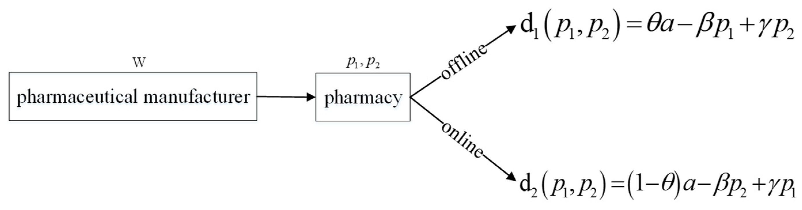
3. Model Descriptions

This paper considers a two-echelon pharmaceutical supply chain that consists of a pharmaceutical manufacturer and a pharmacy with an O2O mixed channel. The pharmacy buys medicines from the pharmaceutical manufacturer and then sells to the patients via offline and online channels. The model is illustrated in Figure 1. The pharmaceutical manufacturer’s unit production cost is $c$ and the sales price is $w$, $w>c$. Additionally, offline unit cost is defined as $c_1$ and offline unit price is defined as $p_1$. Online unit cost is defined as $c_2$ and online unit price is defined as $p_2$. We assume $p_1>w>c_1$ and $p_2>w>c_2$ to ensure that marginal profits of the pharmaceutical manufacturer and pharmacy are positive. The government imposes a wholesale price cap on the pharmaceutical manufacturer, and we set the wholesale price cap as $\overline{w}$.

Similar to Chen et al. and Mukhopadhyay et al., the liner demand functions for the online and offline channels are given as follows [22,36,37]:

$$d_1\left(p_{1,},p_2\right)=\theta \alpha -\beta p_1+\gamma p_2$$

(1)

$$d_2\left(p_1,p_2\right)=\left(1-\theta \right)\alpha -\beta p_2+\gamma p_1$$

(2)

The customers demand from the offline channel is described as $d_1\left(p_1,p_2\right)$, and the customers demand from the online channel is described as $d_2\left(p_1,p_2\right)$. In the demand functions, $\alpha$ represents the base market, $\theta \alpha$ represents the offline market share and $\left(1-\theta \right)\alpha$ represents the online market share. $\beta$ is the self-price sensitivity and $\gamma$ is the cross-price sensitivity. We set $\beta >\gamma$, which means that the self-price sensitivity is higher than the cross-price sensitivity. We assume the pharmaceutical manufacturer and pharmacy are rational and aim to maximize their respective profits. The optimal solutions we derive are unique.

Based on the above demand functions, the pharmaceutical manufacturer’s profit ${\pi }_m\left(w\right)$ is:

$${\pi }_m\left(w\right)=\left(w-c\right)d_1\left(p_1,p_2\right)+\left(w-c\right)d_2\left(p_1,p_2\right)$$

(3)

The first part of this formula represents the pharmaceutical manufacturer’s profit via the offline channel, and the second part of this formula represents the pharmaceutical manufacturer’s profit via the online channel.

We assume that the marginal profit of the offline channel is $m_1=p_1-w$; the marginal profit of the online channel is $m_2=p_2-w$; the pharmaceutical manufacturer’s profit ${\pi }_m\left(w\right)$ can also be expressed as follows:

$${\pi }_m\left(w\right)=\left(w-c\right)\left[\alpha -\left(\beta -\gamma \right)\left(m_1+m_2+2w\right)\right]$$

(4)

The pharmacy’s profit ${\pi }_r\left(p_1,p_2\right)$ is

$${\pi }_r\left(p_1,p_2\right)=\left(p_1-w-c_1\right)d_1\left(p_1,p_2\right)+\left(p_2-w-c_2\right)d_2\left(p_1,p_2\right)$$

(5)

The first part of this formula represents the pharmacy’s profit via the offline channel, and the second part of this formula represents the pharmacy’s profit via the online channel.

Social welfare consists of the patient surplus, pharmaceutical manufacturer’s profit and pharmacy’s profit. Following Chen et al., Cowan and Jin et al., the patient surplus $C_s$ is [3,38,39]

$$\begin{array}{c}{C}_s={{\displaystyle \int }}_0^{\theta \alpha -\beta p_1+\gamma p_2}\left(\frac{\theta \alpha -x+\gamma p_2}{\beta }-p_1\right)d_x+{{\displaystyle \int }}_0^{\left(1-\theta \right)\alpha -\beta p_1+\gamma p_2}\left(\frac{\left(1-\theta \right)\alpha +\gamma p_1-y}{\beta }-p_2\right)d_y\hfill \\ =\frac{{(\theta \alpha -\beta p_1+\gamma p_2)}^2+{[\left(1-\theta \right)\alpha -\beta p_2+\gamma p_1]}^2}{2\beta }\hfill \end{array}$$

(6)

4. Mathematical Models and Equilibrium Analysis

4.1. Base Models

This section explores Pharmaceutical Manufacturer Stackelberg ($\mathrm{MS}$), Pharmacy Stackelberg ($\mathrm{PS}$) and Vertical Nash ($\mathrm{VN}$) models without price cap regulation. The optimal pricing decisions and performances of the pharmaceutical manufacturer and pharmacy will be listed.

4.1.1. Pharmaceutical Manufacturer Stackelberg Model

In the MS model, the pharmaceutical manufacturer is the Stackelberg leader and the pharmacy is the follower. The sequence of events is as follows. Firstly, the pharmacy decides its offline and online retail prices given the pharmaceutical manufacturer’s wholesale price. Then, the pharmaceutical manufacturer decides wholesale price as the response to the pharmacy so as to maximize its own profit. Finally, when customer demand is realized, the pharmaceutical manufacturer and pharmacy will gain their revenues.

4.1.2. Pharmacy Stackelberg Model

In the PS model, the pharmacy is the Stackelberg leader and the pharmaceutical manufacturer is the follower. The sequence of events is as follows. Firstly, the pharmaceutical manufacturer decides wholesale price given the pharmacy’s offline and online retail prices. Then, the pharmacy decides its offline and online prices as a response to the pharmaceutical manufacturer so as to maximize its own profit. Finally, when customer demand is realized, the pharmaceutical manufacturer and pharmacy will gain their revenues.

4.1.3. Vertical Nash Model

In the VN model, the pharmaceutical manufacturer and pharmacy make decisions simultaneously and the order of events is as follows. The pharmacy decides offline and online retail prices to maximize its profits given the pharmaceutical manufacturer’s wholesale price, and the pharmaceutical manufacturer decides wholesale price to maximize its profit given the offline and online retail prices. Finally, when customer demand is realized, the pharmaceutical manufacturer and the pharmacy will gain their revenues.

Based on these functions above, we derive the optimal wholesale prices, the optimal retail prices for the $\mathrm{MS}$,$\mathrm{PS}$ and $\mathrm{VN}$ models, which are summarized in

Table 1. Optimal solutions for base models.

	MS Model	PS Model	VN Model
$w$	$\frac{\alpha }{4\left(\beta -\gamma \right)}+\frac{2c-c_1-c_2}{4}$	$\frac{\alpha }{8\left(\beta -\gamma \right)}+\frac{6c-c_1-c_2}{8}$	$\frac{\alpha }{6\left(\beta -\gamma \right)}+\frac{4c-c_1-c_2}{6}$
$p_1$	$\frac{\left[\left(1+4\theta \right)\beta +\left(5-4\theta \right)\gamma \right]\alpha }{8\left({\beta }^2-{\gamma }^2\right)}$$+\frac{2c+3c_1-c_2}{8}$	$\frac{\left[\left(1+4\theta \right)\beta +\left(5-4\theta \right)\gamma \right]\alpha }{8\left({\beta }^2-{\gamma }^2\right)}$$+\frac{2c+3c_1-c_2}{8}$	$\frac{\left[\left(1+6\theta \right)\beta +\left(7-6\theta \right)\gamma \right]\alpha }{12\left({\beta }^2-{\gamma }^2\right)}$$+\frac{4c+5c_1-c_2}{12}$
$p_2$	$\frac{\left[\left(5-4\theta \right)\beta +\left(1+4\theta \right)\gamma \right]\alpha }{8\left({\beta }^2-{\gamma }^2\right)}$$+\frac{2c-c_1+3c_2}{8}$	$\frac{\left[\left(5-4\theta \right)\beta +\left(1+4\theta \right)\gamma \right]\alpha }{8\left({\beta }^2-{\gamma }^2\right)}$$+\frac{2c-c_1+3c_2}{8}$	$\frac{\left[\left(7-6\theta \right)\beta +\left(1+6\theta \right)\gamma \right]\alpha }{12\left({\beta }^2-{\gamma }^2\right)}$$+\frac{4c-c_1+5c_2}{12}$
${\pi }_m\left(w\right)$	$\frac{{[\alpha -\left(\beta -\gamma \right)\left(2c+c_1+c_2\right)]}^2}{16\left(\beta -\gamma \right)}$	$\frac{{[\alpha -\left(\beta -\gamma \right)\left(2c+c_1+c_2\right)]}^2}{32\left(\beta -\gamma \right)}$	$\frac{{[\alpha -\left(\beta -\gamma \right)\left(2c+c_1+c_2\right)]}^2}{18\left(\beta -\gamma \right)}$
${\pi }_r\left(p_1,p_2\right)$	$\frac{4A+5\beta -3\gamma }{32({\beta }^2-{\gamma }^2)}{\alpha }^2+\frac{B}{8}$$-\frac{{2\mathrm{c}+\mathrm{c}}_1\left(8\theta -3\right)+c_2\left(5-8\theta \right)}{16}\alpha$$+\frac{\beta \left(5c_1{}^2-6c_1{c}_2+5c_2{}^2\right)}{32}$$+\frac{\gamma \left(3c_1^2-10c_1{c}_2+3c_2{}^2\right)}{32}$	$\frac{2A+3\beta -\gamma }{16({\beta }^2-{\gamma }^2)}{\alpha }^2+\frac{B}{4}$$-\frac{{2\mathrm{c}+\mathrm{c}}_1\left(4\theta -1\right)+c_2\left(3-4\theta \right)}{8}\alpha$$+\frac{\beta \left(3c_1{}^2-2c_1{c}_2+3c_2{}^2\right)}{16}$$+\frac{\gamma \left(c_1^2-6c_1{c}_2+c_2{}^2\right)}{16}$	$\frac{9A+13\beta -5\gamma }{72({\beta }^2-{\gamma }^2)}{\alpha }^2+\frac{2B}{9}$$-\frac{{8\mathrm{c}+\mathrm{c}}_1\left(18\theta -5\right)+c_2\left(13-18\theta \right)}{36}\alpha$$+\frac{\beta \left(13c_1{}^2-10c_1{c}_2+13c_2{}^2\right)}{72}$$+\frac{\gamma \left(5c_1^2-26c_1{c}_2+5c_2{}^2\right)}{72}$

where $A=4\left(\beta -\gamma \right){\theta }^2-4\left(\beta -\gamma \right)\theta$, $B=c\left(c+c_1+c_2\right)\left(\beta -\gamma \right)$.

(Please refer to Appendix A.1).

4.2. Price Cap Regulation Models

In the price cap regulation scenario, the government imposes a price cap regulation on the pharmaceutical manufacturer by setting a wholesale price cap ($\overline{w}$). The pharmaceutical manufacturer must decide wholesale price with the constraint, $c<w\le \overline{w}$. We built manufacturer price cap regulation models (MM, PM, VM).

By comparing optimal wholesale prices under different power structures in Table 1, we derive $w^{ps}<w^{vn}<w^{ms}$. Therefore, there are several potential situations when the government imposes a price cap on pharmaceutical manufacturers:

(1)

If the wholesale price cap is higher than the optimal wholesale price in the MS model ($\overline{w}>w^{ms}$), the price cap regulation has no effect on the pharmaceutical supply chain under three power structures.

(2)

If the wholesale price cap is higher than the optimal wholesale price in the VN model and lower than that in the MS model ($w^{vn}<\overline{w}<w^{ms}$), the price cap regulation only has effects on the pharmaceutical supply chain when the pharmaceutical manufacturer is dominant in the market.

(3)

If the wholesale price cap is higher than the optimal wholesale price in the PS model and lower than that in the VN model ($w^{ps}<\overline{w}<w^{vn}$), the price cap regulation affects the pharmaceutical supply chain when the pharmaceutical manufacturer is dominant in the market or the pharmaceutical manufacturer and pharmacy are in a balanced power structure.

(4)

If the wholesale price cap is lower than the optimal wholesale price in the PS model ($\overline{w}<w^{ps}$), the pharmaceutical supply chain under three different power structures will be affected.

The pharmaceutical manufacturer’s profit-maximizing problem $Max{\pi }_m\left(w\right)$ and the pharmacy’s profit-maximizing problem $Max{\pi }_r\left(p_1,p_2\right)$ are

$$\underset{w}{Max}{\pi }_m\left(w\right)=\left(w-c\right)\left[\alpha -\left(\beta -\gamma \right)\left(p_1+p_2\right)\right]$$

(7)

$$\mathrm{s}.\mathrm{t}.w\le \overline{w}$$

$$\underset{p_1,p_2}{Max}{\pi }_r\left(p_1,p_2\right)=\left(p_1-w-c_1\right)d_1+\left(p_2-w-c_2\right)d_2$$

(8)

We derive the optimal wholesale prices, the optimal offline and online retail prices for the MM, PM and VM models, which are summarized in

Table 2. Optimal solutions for price cap regulation models.

Models		$\mathit{w}$	${\mathit{p}}_1$	${\mathit{p}}_2$
MM model	$\overline{w}>w^{ms}$	$\frac{\alpha }{4\left(\beta -\gamma \right)}+\frac{2c-c_1-c_2}{4}$	$\frac{\left[\left(1+4\theta \right)\beta +\left(5-4\theta \right)\gamma \right]\alpha }{8\left({\beta }^2-{\gamma }^2\right)}$$+\frac{2c+3c_1-c_2}{8}$	$\frac{\left[\left(5-4\theta \right)\beta +\left(1+4\theta \right)\gamma \right]\alpha }{8\left({\beta }^2-{\gamma }^2\right)}$$+\frac{2c-c_1+3c_2}{8}$
	$w^{vn}<\overline{w}<w^{ms}$	$\overline{w}$	$\frac{\left[\left(1-\theta \right)\gamma +\theta \beta \right]\alpha }{2\left({\beta }^2-{\gamma }^2\right)}+\frac{\overline{w}+c_1}{2}$	$\frac{\left[\left(1-\theta \right)\beta +\theta \gamma \right]\alpha }{2\left({\beta }^2-{\gamma }^2\right)}+\frac{\overline{w}+c_2}{2}$
	$w^{ps}<\overline{w}<w^{vn}$	$\overline{w}$	$\frac{\left[\left(1-\theta \right)\gamma +\theta \beta \right]\alpha }{2\left({\beta }^2-{\gamma }^2\right)}+\frac{\overline{w}+c_1}{2}$	$\frac{\left[\left(1-\theta \right)\beta +\theta \gamma \right]\alpha }{2\left({\beta }^2-{\gamma }^2\right)}+\frac{\overline{w}+c_2}{2}$
	$\overline{w}<w^{ps}$	$\overline{w}$	$\frac{\left[\left(1-\theta \right)\gamma +\theta \beta \right]\alpha }{2\left({\beta }^2-{\gamma }^2\right)}+\frac{\overline{w}+c_1}{2}$	$\frac{\left[\left(1-\theta \right)\beta +\theta \gamma \right]\alpha }{2\left({\beta }^2-{\gamma }^2\right)}+\frac{\overline{w}+c_2}{2}$
PM model	$\overline{w}>w^{ms}$	$\frac{\alpha }{8\left(\beta -\gamma \right)}+\frac{6c-c_1-c_2}{8}$	$\frac{\left[\left(1+4\theta \right)\beta +\left(5-4\theta \right)\gamma \right]\alpha }{8\left({\beta }^2-{\gamma }^2\right)}$$+\frac{2c+3c_1-c_2}{8}$	$\frac{\left[\left(5-4\theta \right)\beta +\left(1+4\theta \right)\gamma \right]\alpha }{8\left({\beta }^2-{\gamma }^2\right)}$$+\frac{2c-c_1+3c_2}{8}$
	$w^{vn}<\overline{w}<w^{ms}$	$\frac{\alpha }{8\left(\beta -\gamma \right)}+\frac{6c-c_1-c_2}{8}$	$\frac{\left[\left(1+4\theta \right)\beta +\left(5-4\theta \right)\gamma \right]\alpha }{8\left({\beta }^2-{\gamma }^2\right)}$$+\frac{2c+3c_1-c_2}{8}$	$\frac{\left[\left(5-4\theta \right)\beta +\left(1+4\theta \right)\gamma \right]\alpha }{8\left({\beta }^2-{\gamma }^2\right)}$$+\frac{2c-c_1+3c_2}{8}$
	$w^{ps}<\overline{w}<w^{vn}$	$\frac{\alpha }{8\left(\beta -\gamma \right)}+\frac{6c-c_1-c_2}{8}$	$\frac{\left[\left(1+4\theta \right)\beta +\left(5-4\theta \right)\gamma \right]\alpha }{8\left({\beta }^2-{\gamma }^2\right)}$$+\frac{2c+3c_1-c_2}{8}$	$\frac{\left[\left(5-4\theta \right)\beta +\left(1+4\theta \right)\gamma \right]\alpha }{8\left({\beta }^2-{\gamma }^2\right)}$$+\frac{2c-c_1+3c_2}{8}$
	$\overline{w}<w^{ps}$	$\overline{w}$	$\frac{\left[\left(1-\theta \right)\gamma +\theta \beta \right]\alpha }{2\left({\beta }^2-{\gamma }^2\right)}+\frac{\overline{w}+c_1}{2}$	$\frac{\left[\left(1-\theta \right)\beta +\theta \gamma \right]\alpha }{2\left({\beta }^2-{\gamma }^2\right)}+\frac{\overline{w}+c_2}{2}$
VM model	$\overline{w}>w^{ms}$	$\frac{\alpha }{6\left(\beta -\gamma \right)}+\frac{4c-c_1-c_2}{6}$	$\frac{\left[\left(1+6\theta \right)\beta +\left(7-6\theta \right)\gamma \right]\alpha }{12\left({\beta }^2-{\gamma }^2\right)}$$+\frac{4c+5c_1-c_2}{12}$	$\frac{\left[\left(7-6\theta \right)\beta +\left(1+6\theta \right)\gamma \right]\alpha }{12\left({\beta }^2-{\gamma }^2\right)}$$+\frac{4c-c_1+5c_2}{12}$
	$w^{vn}<\overline{w}<w^{ms}$	$\frac{\alpha }{6\left(\beta -\gamma \right)}+\frac{4c-c_1-c_2}{6}$	$\frac{\left[\left(1+6\theta \right)\beta +\left(7-6\theta \right)\gamma \right]\alpha }{12\left({\beta }^2-{\gamma }^2\right)}$$+\frac{4c+5c_1-c_2}{12}$	$\frac{\left[\left(7-6\theta \right)\beta +\left(1+6\theta \right)\gamma \right]\alpha }{12\left({\beta }^2-{\gamma }^2\right)}$$+\frac{4c-c_1+5c_2}{12}$
	$w^{ps}<\overline{w}<w^{vn}$	$\overline{w}$	$\frac{\left[\left(1+6\theta \right)\beta +\left(7-6\theta \right)\gamma \right]\alpha }{12\left({\beta }^2-{\gamma }^2\right)}$$+\frac{4c+5c_1-c_2}{12}$	$\frac{\left[\left(7-6\theta \right)\beta +\left(1+6\theta \right)\gamma \right]\alpha }{12\left({\beta }^2-{\gamma }^2\right)}$$+\frac{4c-c_1+5c_2}{12}$
	$\overline{w}<w^{ps}$	$\overline{w}$	$\frac{\left[\left(1+6\theta \right)\beta +\left(7-6\theta \right)\gamma \right]\alpha }{12\left({\beta }^2-{\gamma }^2\right)}$$+\frac{4c+5c_1-c_2}{12}$	$\frac{\left[\left(7-6\theta \right)\beta +\left(1+6\theta \right)\gamma \right]\alpha }{12\left({\beta }^2-{\gamma }^2\right)}$$+\frac{4c-c_1+5c_2}{12}$

(Please refer to Appendix A.2).

Based on the optimal solutions in Table 2, we obtain the optimal profits for three regulation models, which are summarized in

Table 3. Optimal profits for price cap regulation models.

Models		${\mathit{\pi }}_{\mathit{m}}\left(\mathit{w}\right)$	${\mathit{\pi }}_{\mathit{r}}\left({\mathit{p}}_1,{\mathit{p}}_2\right)$
MM model	$\overline{w}>w^{ms}$	$\frac{{[\alpha -\left(\beta -\gamma \right)\left(2c+c_1+c_2\right)]}^2}{16\left(\beta -\gamma \right)}$	$\frac{16\left(\beta -\gamma \right){\theta }^2-16\left(\beta -\gamma \right)\theta +5\beta -3\gamma }{32\left({\beta }^2-{\gamma }^2\right)}{\alpha }^2$$-\frac{2c+c_1\left(8\theta -3\right)+c_2\left(5-8\theta \right)}{16}\alpha$$+\frac{c\left(c+c_1+c_2\right)\left(\beta -\gamma \right)}{8}$$+\frac{\beta \left(5c_1{}^2-6c_1{c}_2+5c_2{}^2\right)+\gamma \left(3c_1{}^2-10c_1{c}_2+3c_2{}^2\right)}{32}$
	$w^{vn}<\overline{w}<w^{ms}$	$\frac{\left(\overline{w}-c\right)\left[a-\left(2\overline{w}+c_1+c_2\right)\left(\beta -\gamma \right)\right]}{2}$	$\left[\frac{[\left(\theta -1\right)\theta }{2\left(\beta +\gamma \right)}+\frac{\beta }{4\left({\beta }^2-{\gamma }^2\right)}\right]{\alpha }^2$$+\frac{\beta -\gamma }{2}{\overline{w}}^2-\frac{\alpha -\left(c_1+c_2\right)\left(\beta -\gamma \right)}{2}\overline{w}$$+\frac{c_1{}^2+c_2{}^2}{4}\beta -\frac{\theta \left(c_1-c_2\right)+c_2}{2}\alpha$
	$w^{ps}<\overline{w}<w^{vn}$	$\frac{\left(\overline{w}-c\right)\left[a-\left(2\overline{w}+c_1+c_2\right)\left(\beta -\gamma \right)\right]}{2}$	$\left[\frac{[\left(\theta -1\right)\theta }{2\left(\beta +\gamma \right)}+\frac{\beta }{4\left({\beta }^2-{\gamma }^2\right)}\right]{\alpha }^2$$+\frac{\beta -\gamma }{2}{\overline{w}}^2-\frac{\alpha -\left(c_1+c_2\right)\left(\beta -\gamma \right)}{2}\overline{w}$$+\frac{c_1{}^2+c_2{}^2}{4}\beta -\frac{\theta \left(c_1-c_2\right)+c_2}{2}\alpha$
	$\overline{w}<w^{ps}$	$\frac{\left(\overline{w}-c\right)\left[a-\left(2\overline{w}+c_1+c_2\right)\left(\beta -\gamma \right)\right]}{2}$	$\left[\frac{[\left(\theta -1\right)\theta }{2\left(\beta +\gamma \right)}+\frac{\beta }{4\left({\beta }^2-{\gamma }^2\right)}\right]{\alpha }^2$$+\frac{\beta -\gamma }{2}{\overline{w}}^2-\frac{\alpha -\left(c_1+c_2\right)\left(\beta -\gamma \right)}{2}\overline{w}$$+\frac{c_1{}^2+c_2{}^2}{4}\beta -\frac{\theta \left(c_1-c_2\right)+c_2}{2}\alpha$
PM model	$\overline{w}>w^{ms}$	$\frac{{[\alpha -\left(\beta -\gamma \right)\left(2c+c_1+c_2\right)]}^2}{32\left(\beta -\gamma \right)}$	$\frac{8\left(\beta -\gamma \right){\theta }^2-8\left(\beta -\gamma \right)\theta +3\beta -\gamma }{16\left({\beta }^2-{\gamma }^2\right)}{\alpha }^2$$-\frac{2c+c_1\left(4\theta -1\right)+c_2\left(3-4\theta \right)}{8}\alpha$$+\frac{c\left(c+c_1+c_2\right)\left(\beta -\gamma \right)}{4}$$+\frac{\beta \left(3c_1{}^2-2c_1{c}_2+3c_2{}^2\right)+\gamma \left(c_1{}^2-6c_1{c}_2+c_2{}^2\right)}{16}$
	$w^{vn}<\overline{w}<w^{ms}$	$\frac{{[\alpha -\left(\beta -\gamma \right)\left(2c+c_1+c_2\right)]}^2}{32\left(\beta -\gamma \right)}$	$\frac{8\left(\beta -\gamma \right){\theta }^2-8\left(\beta -\gamma \right)\theta +3\beta -\gamma }{16\left({\beta }^2-{\gamma }^2\right)}{\alpha }^2$$-\frac{2c+c_1\left(4\theta -1\right)+c_2\left(3-4\theta \right)}{8}\alpha$$+\frac{c\left(c+c_1+c_2\right)\left(\beta -\gamma \right)}{4}$$+\frac{\beta \left(3c_1{}^2-2c_1{c}_2+3c_2{}^2\right)+\gamma \left(c_1{}^2-6c_1{c}_2+c_2{}^2\right)}{16}$
	$w^{ps}<\overline{w}<w^{vn}$	$\frac{{[\alpha -\left(\beta -\gamma \right)\left(2c+c_1+c_2\right)]}^2}{32\left(\beta -\gamma \right)}$	$\frac{8\left(\beta -\gamma \right){\theta }^2-8\left(\beta -\gamma \right)\theta +3\beta -\gamma }{16\left({\beta }^2-{\gamma }^2\right)}{\alpha }^2$$-\frac{2c+c_1\left(4\theta -1\right)+c_2\left(3-4\theta \right)}{8}\alpha$$+\frac{c\left(c+c_1+c_2\right)\left(\beta -\gamma \right)}{4}$$+\frac{\beta \left(3c_1{}^2-2c_1{c}_2+3c_2{}^2\right)+\gamma \left(c_1{}^2-6c_1{c}_2+c_2{}^2\right)}{16}$
	$\overline{w}<w^{ps}$	$\frac{\left(\overline{w}-c\right)\left[a-\left(2\overline{w}+c_1+c_2\right)\left(\beta -\gamma \right)\right]}{2}$	$\left[\frac{[\left(\theta -1\right)\theta }{2\left(\beta +\gamma \right)}+\frac{\beta }{4\left({\beta }^2-{\gamma }^2\right)}\right]{\alpha }^2+\frac{\beta -\gamma }{2}{\overline{w}}^2$$-\frac{\alpha -\left(c_1+c_2\right)\left(\beta -\gamma \right)}{2}\overline{w}+\frac{c_1{}^2+c_2{}^2}{4}\beta -\frac{\theta \left(c_1-c_2\right)+c_2}{2}\alpha$
VM model	$\overline{w}>w^{ms}$	$\frac{{[\alpha -\left(\beta -\gamma \right)\left(2c+c_1+c_2\right)]}^2}{18\left(\beta -\gamma \right)}$	$\frac{36\left(\beta -\gamma \right){\theta }^2-36\left(\beta -\gamma \right)\theta +13\beta -5\gamma }{72\left({\beta }^2-{\gamma }^2\right)}{\alpha }^2$$-\frac{8c+c_1\left(18\theta -5\right)+c_2\left(13-18\theta \right)}{36}\alpha$$+\frac{2c\left(c+c_1+c_2\right)\left(\beta -\gamma \right)}{9}$$+\frac{\beta \left(13c_1{}^2-10c_1{c}_2+13c_2{}^2\right)+\gamma \left(5c_1{}^2-26c_1{c}_2+5c_2{}^2\right)}{72}$
	$w^{vn}<\overline{w}<w^{ms}$	$\frac{{[\alpha -\left(\beta -\gamma \right)\left(2c+c_1+c_2\right)]}^2}{18\left(\beta -\gamma \right)}$	$\frac{36\left(\beta -\gamma \right){\theta }^2-36\left(\beta -\gamma \right)\theta +13\beta -5\gamma }{72\left({\beta }^2-{\gamma }^2\right)}{\alpha }^2$$-\frac{8c+c_1\left(18\theta -5\right)+c_2\left(13-18\theta \right)}{36}\alpha$$+\frac{2c\left(c+c_1+c_2\right)\left(\beta -\gamma \right)}{9}$$+\frac{\beta \left(13c_1{}^2-10c_1{c}_2+13c_2{}^2\right)+\gamma \left(5c_1{}^2-26c_1{c}_2+5c_2{}^2\right)}{72}$
	$w^{ps}<\overline{w}<w^{vn}$	$\frac{\left(\overline{w}-c\right)\left[\alpha -\left(2c+c_1+c_2\right)\left(\beta -\gamma \right)\right]}{3}$	$\left[\frac{\left(7-6\theta \right)\left(5\beta -\gamma \right)+\left(1+6\theta \right)\left(5\gamma -\beta \right)}{144({\beta }^2-{\gamma }^2)}+\frac{\left(2\theta -1\right)\theta }{4\left(\beta +\gamma \right)}\right]{\alpha }^2$$+\frac{\left(4c-7c_1-c_2\right)\left(6\theta -1\right)+\left(4c-c_1-7c_2\right)\left(5-6\theta \right)}{144}\alpha$$-\frac{\left(4c+5c_1-c_2\right)\left(1+6\theta \right)+\left(4c-c_1+5c_2\right)\left(7-6\theta \right)}{144}\alpha$$-\frac{\left(4c-7c_1-c_2\right)\left(4c-c_1+5c_2\right)}{144}\gamma -\frac{\left(4c-c_1-7c_2\right)\left(4c+5c_1-c_2\right)}{144}\gamma$$-\frac{\left(4c-7c_1-c_2\right)\left(4c+5c_1-c_2\right)}{144}\beta -\frac{\left(4c-c_1-7c_2\right)\left(4c-c_1+5c_2\right)}{144}\beta$$-\left[\frac{1}{3}\alpha -\frac{2c+c_1+c_2}{3}\left(\beta -\gamma \right)\right]\overline{w}$
	$\overline{w}<w^{ps}$	$\frac{\left(\overline{w}-c\right)\left[\alpha -\left(2c+c_1+c_2\right)\left(\beta -\gamma \right)\right]}{3}$	$\left[\frac{\left(7-6\theta \right)\left(5\beta -\gamma \right)+\left(1+6\theta \right)\left(5\gamma -\beta \right)}{144({\beta }^2-{\gamma }^2)}+\frac{\left(2\theta -1\right)\theta }{4\left(\beta +\gamma \right)}\right]{\alpha }^2$$+\frac{\left(4c-7c_1-c_2\right)\left(6\theta -1\right)+\left(4c-c_1-7c_2\right)\left(5-6\theta \right)}{144}\alpha$$-\frac{\left(4c+5c_1-c_2\right)\left(1+6\theta \right)+\left(4c-c_1+5c_2\right)\left(7-6\theta \right)}{144}\alpha$$-\frac{\left(4c-7c_1-c_2\right)\left(4c+5c_1-c_2\right)}{144}\beta -\frac{\left(4c-c_1-7c_2\right)\left(4c-c_1+5c_2\right)}{144}\beta$$-\left[\frac{1}{3}\alpha -\frac{2c+c_1+c_2}{3}\left(\beta -\gamma \right)\right]\overline{w}$

.

5. Effects of the Power Structures

In this section, we study how power structures affect the pricing decisions, performances, and social welfare of the regulated pharmaceutical supply chain. We present the following propositions.

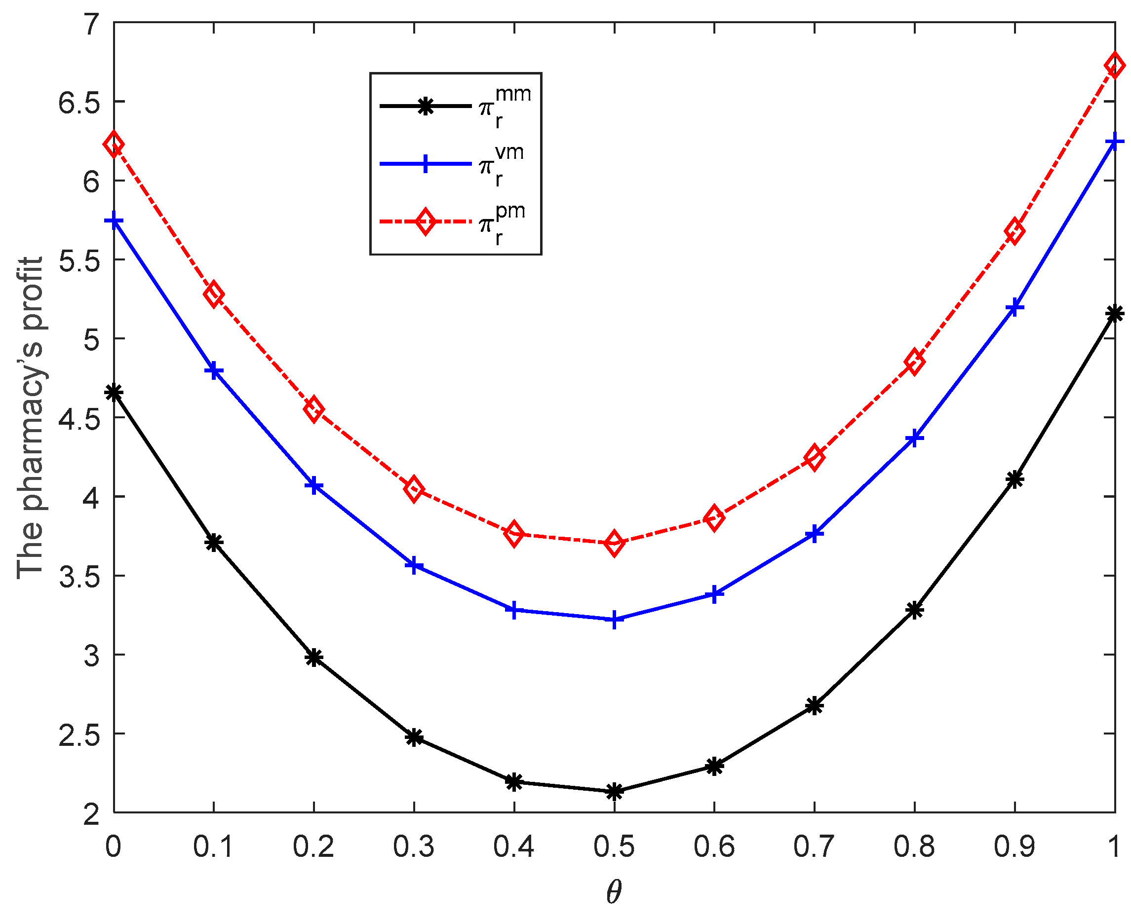
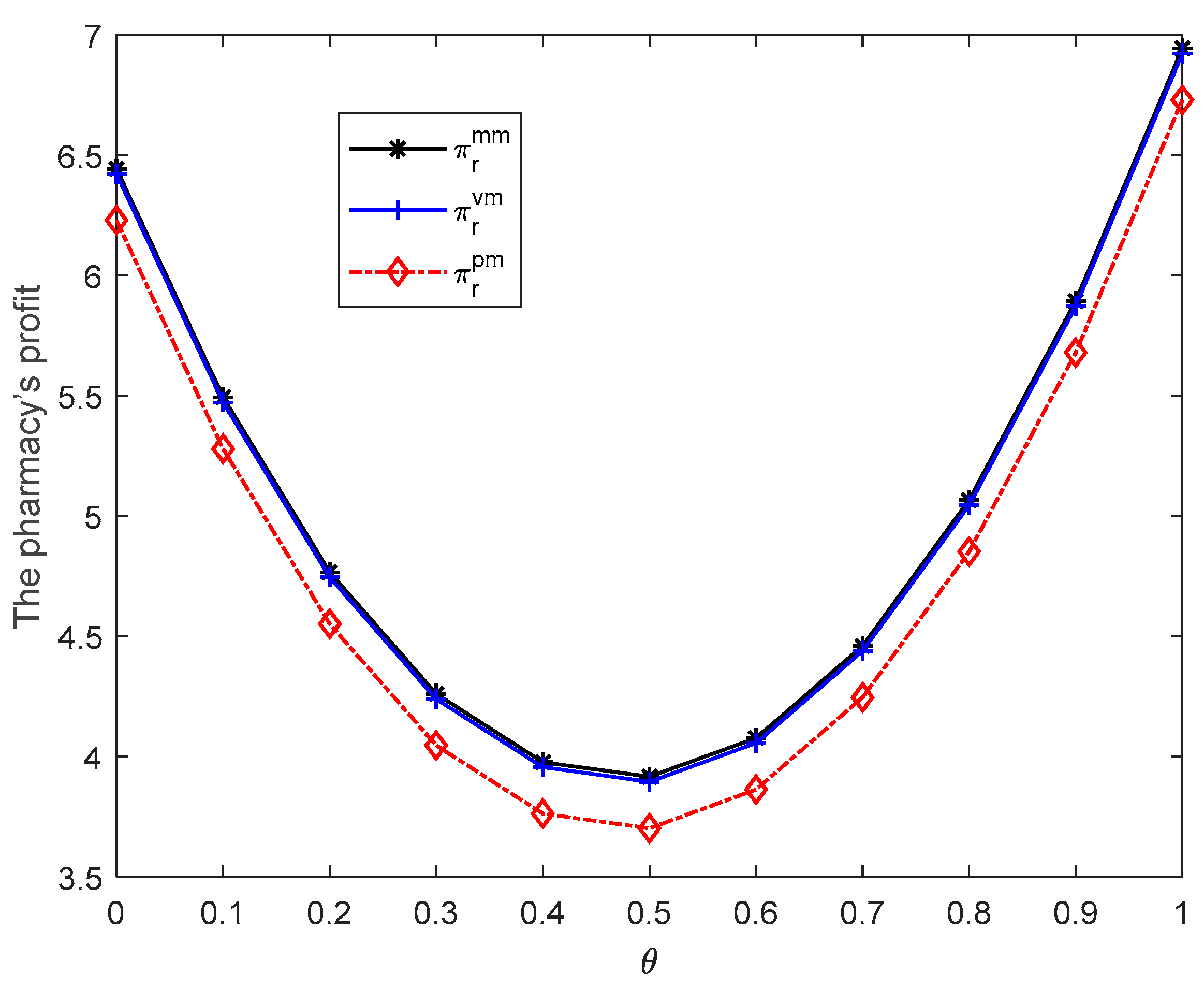
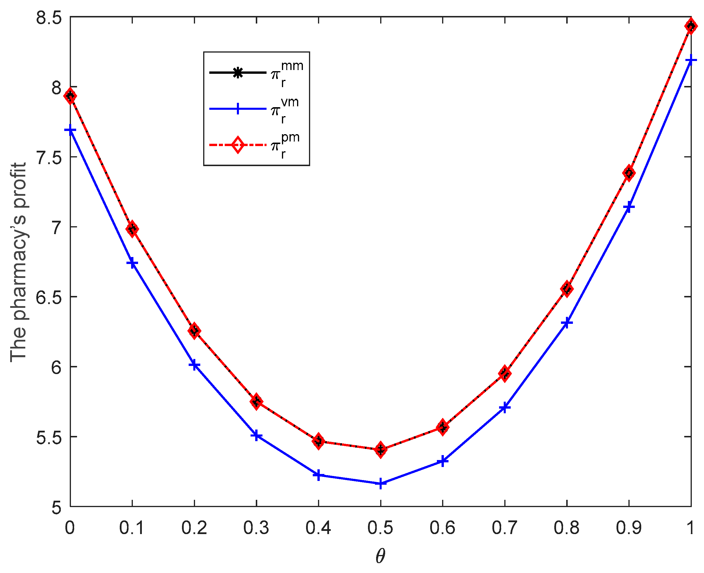
5.1. Effects of Power Structures on the Pricing and Performance

Proposition 1.

If$\overline{w}>w^{ms}$, then (i)$w^{mm}>w^{vm}>w^{pm}$,$p_1^{mm}=p_1^{pm}>p_1^{vm}$,$p_2^{mm}=p_2^{pm}{p}_2^{vm}$; (ii)${\pi }_m^{mm}>{\pi }_m^{vm}>{\pi }_m^{pm}$,${\pi }_r^{pm}>{\pi }_r^{vm}>{\pi }_r^{mm}$,${\pi }^{pm}={\pi }^{mm}<{\pi }^{vm}$.

This proposition shows that when the wholesale price cap is higher than the optimal wholesale price in the MS model ($\overline{w}>w^{ms}$), the influence of power structures on the drug supply chain will be consistent with previous research results [22,27]. Where there is no price cap regulation, pharmaceutical firms that have more power than other members will set higher prices for higher profits. However, the fierce market competition will improve the total profit of the supply chain.

Proposition 2.

If$w^{vn}<\overline{w}<w^{ms}$, then$w^{mm}>w^{vm}>w^{pm}$,$p_1^{pm}>p_1^{mm}>p_1^{vm}$,$p_2^{pm}>p_2^{mm}>p_2^{vm}$,${\pi }_m^{mm}>{\pi }_m^{vm}>{\pi }_m^{pm}$.

Proposition 2 shows that when the wholesale price cap is higher than the optimal wholesale price in the VN model and lower than the optimal wholesale price in the MS model ($w^{vn}<\overline{w}<w^{ms}$), the wholesale price will be restricted in the manufacturer-dominated market. The manufacturer’s prices and profits will be the highest in the manufacturer-dominant market. The optimal offline and online retail prices in the PM model will be higher than those in the MM model, which can be explained by the fact that the pharmaceutical manufacturer is constrained by a lower wholesale price in the MM model, so its retail prices are correspondingly reduced. Besides, the optimal offline and online retail prices in the VM model will be the lowest. In a world, when the wholesale price cap is relatively high, power structures have a more significant impact on the pharmaceutical supply chain than the price cap regulation.

Proposition 3.

If$w^{ps}<\overline{w}<w^{vn}$, then$w^{mm}=w^{vm}>w^{pm}$,$p_1^{pm}>p_1^{vm}>p_1^{mm}$,$p_2^{pm}>p_2^{vm}>p_2^{mm}$,${\pi }_m^{mm}>{\pi }_m^{vm}>{\pi }_m^{pm}$.

This proposition indicates that when the wholesale price cap is higher than the optimal wholesale price in the PS model and lower than the optimal wholesale price in the VN model ($w^{ps}<\overline{w}<w^{vn}$), the optimal wholesale price in the MM model will be equal to that in the VM model, higher than that in the PM model. The optimal offline and online retail prices will be the highest in the PM model, in the middle in the VM model, and lowest in the MM model. This is easy to explain the retail prices decrease correspondingly as the wholesale price is restricted in MM market and VM market. In addition, the pharmaceutical manufacturer’s optimal profit will be the highest in the MM model, in the middle in the VM model, and lowest in the PM model. It means that the pharmaceutical manufacturer gains more profit when it has more power in the market, which is consistent with the scenario when there is no price cap.

Proposition 4.

If$\overline{w}<w^{ps}$, then$w^{mm}=w^{vm}=w^{pm}$,$p_1^{pm}=p_1^{mm}<p_1^{vm}$,$p_2^{pm}=p_2^{mm}<p_2^{vm}$,${\pi }_m^{mm}={\pi }_m^{pm}>{\pi }_m^{vm}$.

According to this proposition, if the wholesale price is lower than the optimal wholesale price in the PS model ($\overline{w}<w^{ps}$), the wholesale prices in different power structures will be equal. The optimal offline and online retail prices in the PM model will equal that in the MM model, lower than that in the VM model. It indicates that the pharmacy sets higher offline and online retail prices in the balanced power structure, which is contrary to the conclusion when there is no price cap regulation. Moreover, the pharmaceutical manufacturer’s optimal profit in the MM model will equal that in the RM model, higher than that in the VM model. It shows that the pharmaceutical manufacturer gains more profit in the manufacturer Stackelberg and pharmacy Stackelberg markets.

The optimal profits of pharmacy are derived in Table 3. We use a numerical example to demonstrate the impact of power structures on the performance of the pharmacy when the government imposes a price cap on the pharmaceutical manufacturer. In the example, we set $\beta =3$,$\gamma =1.5$, $\alpha =10$, $c_1=0.1$,$c_2=0.2$,$c=0.01$. Figure 2, Figure 3, Figure 4 and Figure 5 show the profits of the pharmacy in different power structures. When $w^{vn}<\overline{w}<w^{ms}$, we set $\overline{w}=1.5$. When $w^{ps}<\overline{w}<w^{vn}$, we set $\overline{w}=0.9$. When $\overline{w}<w^{ps}$, we set $\overline{w}=0.5$.

Figure 2 shows that if $w^{vn}<\overline{w}<w^{ms}$, the pharmacy’s optimal profit will be the highest when the pharmacy is dominant in the market, in the middle when the pharmaceutical manufacturer and pharmacy are in a balanced market, and lowest when the pharmaceutical manufacturer has dominant power force. It means that the pharmacy still gains more profits when it has more power in the market in this situation.

Figure 3 illustrates that if $w^{ps}<\overline{w}<w^{vn}$, the pharmacy’s optimal profit will be the highest when the pharmaceutical manufacturer is the Stackelberg leader in the market; the pharmacy’s optimal profit will be in the middle when the pharmaceutical manufacturer and pharmacy are in a balanced market; and the pharmacy’s optimal profit will be the lowest when the pharmacy is dominant in the market. It means that the pharmacy’s dominant force in the market is not conducive to gain more profit in this case.

Figure 4 illustrates that if $\overline{w}<w^{ps}$, the pharmacy’s optimal profit in the PM model will equal that in the MM model, higher than that in a balanced market. Combining the above, the pharmaceutical manufacturer’s profit is also the lowest in a balanced market structure. It means that the price cap regulation may be harmful to the establishment of a fair market environment in this situation. Therefore, the government should take the power structure as an important consideration when formulating price cap regulations.

5.2. Effects of Power Structure on Social Welfare

In this subsection, we explore how power structures affect social welfare when the government imposes a price cap on the pharmaceutical manufacturer.

Proposition 5.

If$\overline{w}>w^{ms}$, then$W^{mm}=W^{pm}<W^{vm}$.

Proposition 5 shows that if the price cap regulation does not work, social welfare in pharmaceutical-manufacturer-dominated and pharmacy-dominated markets will be equal, rather lower than that in the balanced power structure. In other words, when there is no price cap, more intense competition drives the prices down and enhances social welfare.

When the wholesale price cap is lower than the optimal wholesale price in the MS model ($\overline{w}<w^{ms}$), social welfare in three different power structures is shown in Figure 5, Figure 6 and Figure 7.

Figure 5 shows that if the wholesale price cap is higher than the optimal wholesale price in the VN model and lower than the optimal wholesale price in the MS model ($w^{vn}<\overline{w}<w^{ms}$), the optimal social welfare will be the highest when the pharmaceutical manufacturer and pharmacy are in a balanced market, in the middle when the pharmaceutical manufacturer is dominant in the market and lowest when the pharmacy has dominant market power. Compared with Proposition 5, we find that social welfare in the manufacturer-dominated market increases. It can be explained that the wholesale price is restricted and the retail prices are correspondingly reduced, so social welfare is improved.

Figure 6 illustrates that if the wholesale price cap is higher than the optimal wholesale price in the PS model and lower than the optimal wholesale price in the VN model ($w^{ps}<\overline{w}<w^{vn}$), the optimal social welfare will be the highest when the pharmaceutical manufacturer is the leader in the market, the optimal social welfare will be in the middle when the pharmaceutical manufacturer and pharmacy are in a balanced market, and the optimal social welfare will be the lowest when the pharmacy is dominant in the market.

Figure 7 illustrates that if the wholesale price cap is lower than the optimal wholesale price in the PS model ($\overline{w}<w^{ps}$), the optimal social welfare in the PS model will be equal to that in the MM model, higher than the optimal social welfare when pharmaceutical supply chain members are in a balanced market. It means that when the wholesale price cap is very low, the fierce market competition leads to the decrease in social welfare, which is the opposite of a situation where there is no price cap regulation.

6. Effects of the Price Cap Regulation

In this section, we explore that how the price cap regulation affects the performance and social welfare of the pharmaceutical supply chain.

6.1. Effects of Price Cap Regulation on Performance

Proposition 6.

For the MM model, if$\overline{w}<w^{ms}$, then the pharmaceutical manufacturer’s profit will increase in$\overline{w}$andthe pharmacy’s profit will decrease in$\overline{w}$. For the PM model, if$\overline{w}<w^{ps}$, then the pharmaceutical manufacturer’s profit will increase in$\overline{w}$, the pharmacy’s profit will decrease in$\overline{w}$. For the VM model, if$\overline{w}<w^{vn}$,the pharmaceutical manufacturer’s profit will increase in$\overline{w}$, the pharmacy’s profit will decrease in$\overline{w}$.

Proposition 6 indicates that no matter what power structure the pharmaceutical supply chain is in, the higher the restricted wholesale price cap, the higher the profit of the pharmaceutical manufacturer. Conversely, when the restricted wholesale price cap is lower, the profit of the pharmacy is higher.

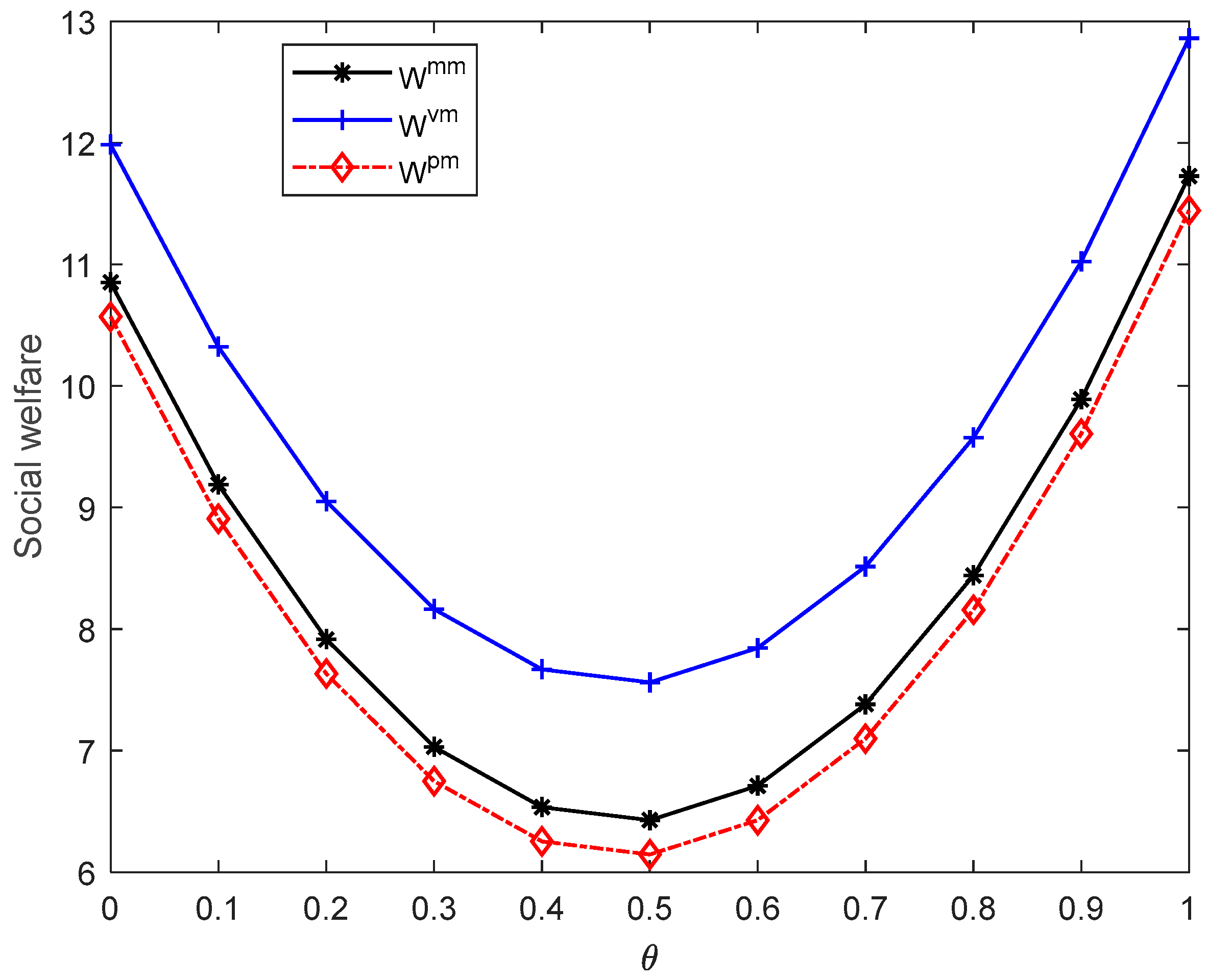
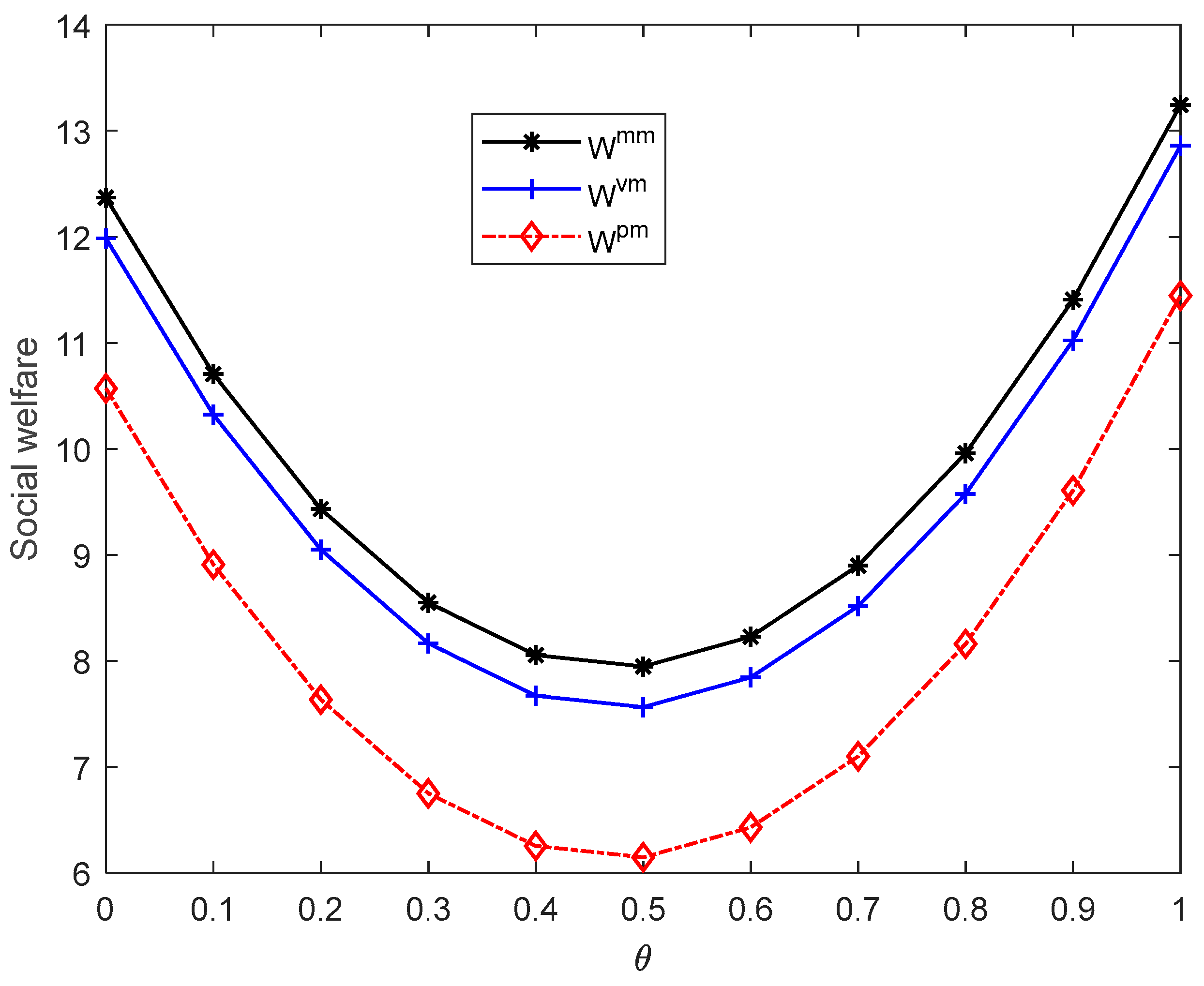
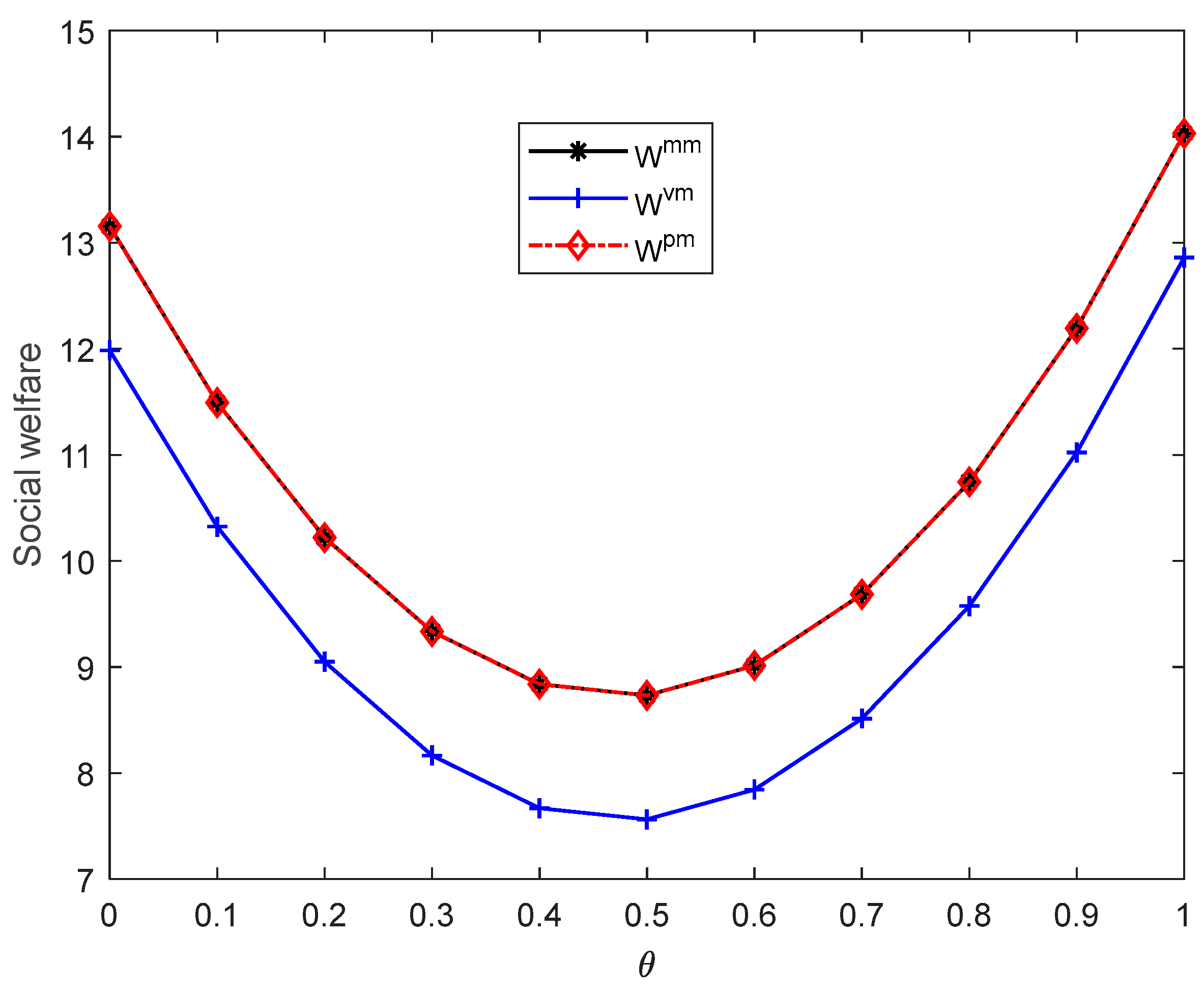
6.2. Effects of Price Cap Regulation on Social Welfare

In this subsection, we explore the impact of the price cap regulation on social welfare, and the proposition is presented below.

Proposition 7.

For the MM model, if$\overline{w}<w^{ms}$, then social welfare will decrease in$\overline{w}$. For the PM model, if$\overline{w}<w^{ps}$, then social welfare will decrease in$\overline{w}$. For the VM model, if$\overline{w}<w^{vn}$,the social welfare will be dependent on$\overline{w}$.

Proposition 7 shows that when the pharmaceutical manufacturer dominates the market or pharmacy dominates the market, the restricted wholesale price cap set by the government is negatively related to social welfare. Additionally, when the pharmaceutical firms are in a balanced market structure, the restricted price cap has no effect on social welfare. Price cap regulations aim to improve patient welfare and social welfare; in order to achieve this goal, the power structure should also be considered.

7. Conclusions and Future Research

In this paper, we studied a two-echelon regulated pharmaceutical supply chain consisting of a pharmaceutical manufacturer and a pharmacy with an O2O mixed channel. We defined three different supply chain power structures: Pharmaceutical Manufacturer-Stackelberg, Pharmacy Stackelberg and Nash equilibrium. Optimal pricing, profits and social welfare are derived in different power structures by game theory. Then we analyze the impacts of power relationship and price cap regulation on decision making, economic performance and social welfare of the pharmaceutical supply chain. The main findings are as follows:

(1)

When the price cap is in different ranges, the influence of the power structure on the economic and social benefits of the pharmaceutical supply chain is different. When the wholesale price cap is higher than the optimal wholesale price in the MS model, the price cap regulation will not work in the supply chain in three different power structures. The pharmaceutical manufacturer and pharmacy can gain more profits when they dominate the market, whereas the balanced power relationship between supply chain members can improve the total profit and social welfare. When the wholesale price cap is lower than the optimal price cap, the pharmaceutical manufacturer will still gain higher profits when it has more market power over other supply chain members. However, for pharmacies, market power cannot ensure that they can make more profits with the influence of the restricted wholesale price cap. Therefore, leading pharmacies may resist the price cap regulation; as a result, this increases the risk of policy failure. The government may consider subsidizing dominated pharmacies when implementing price cap regulation. When the price cap is very low, an interesting discovery is presented. Price cap regulation might harm financial performance and social welfare when pharmaceutical firms are in a balanced power structure. Thus, when the wholesale price cap is lower than a certain threshold, price cap regulation might be detrimental to creating a fair market environment for enterprises.

(2)

We find the wholesale price cap is an important parameter that affects financial performance and social welfare of the pharmaceutical supply chain. Regardless of the power structures, the pharmaceutical manufacturer’s profit is positively correlated with restricted wholesale price. The pharmacy’s profit is negatively correlated with the restricted wholesale price. In addition, social welfare in pharmaceutical manufacturer Stackelberg and pharmacy Stackelberg markets is negatively correlated with the restricted wholesale price, and social welfare in the balanced market is dependent on the restricted wholesale price.

(3)

Overall, this paper provides insights into the pricing decisions of pharmaceutical companies under different power structures. In addition, it also provides a decision-making basis for the government to make price limit policies in different power markets.

Similar to the existing literature, some research limitations exist in our work. For example, our model only discusses a supply chain consisting of one pharmaceutical manufacturer and one pharmacy with O2O channels. An important extension is to explore the complex pharmaceutical supply chain with multiple channels and multiple manufacturers and pharmacies [40,41]. Additionally, our model sets by using linear demand. Another important extension is to consider stochastic demand [22,25]. Finally, we consider pharmaceutical manufacturer price cap regulation. Future research will consider pharmacy price cap regulation and linkage price cap regulation [3]. Power relationships in the pharmaceutical supply chain with different price cap regulations may yield important insights for policymakers.

References

1. Abbott, T.A., III. Price regulation in the pharmaceutical industry: Prescription or placebo? J. Health Econ. 1995, 14, 551–565. [Google Scholar] [CrossRef]
2. Brekke, K.R.; Grasdal, A.L.; Holmås, T.H. Regulation and pricing of pharmaceuticals: Reference pricing or price cap regulation? Eur. Econ. Rev. 2006, 53, 170–185. [Google Scholar] [CrossRef]
3. Cai, G.; Zhang, Z.G.; Zhang, M. Game theoretical perspectives on dual-channel supply chain competition with price discounts and pricing schemes. Int. J. Prod. Econ. 2009, 117, 80–96. [Google Scholar] [CrossRef]
4. Chen, J.; Zhang, H.; Sun, Y. Implementing coordination contracts in a manufacturer Stackelberg dual-channel supply chain. Omega 2012, 40, 571–583. [Google Scholar] [CrossRef]
5. Chen, X.; Li, L.; Zhou, M. Manufacturer’s pricing strategy for supply chain with warranty period-dependent demand. Omega 2012, 40, 807–816. [Google Scholar] [CrossRef]
6. Chen, X.; Li, S.S.; Wang, X. Evaluating the effects of quality regulations on the pharmaceutical supply chain. Int. J. Prod. Econ. 2020, 230, 107770. [Google Scholar] [CrossRef]
7. Chen, X.; Luo, Z.; Wang, X.J. Impact of efficiency, investment, and competition on low carbon manufacturing. J. Clean. Prod. 2017, 143, 388–400. [Google Scholar] [CrossRef] [Green Version]
8. Chen, X.; Wang, X. Free or bundled: Channel selection decisions under different power structures. Omega 2015, 53, 11–20. [Google Scholar] [CrossRef]
9. Chen, X.; Wang, X.; Chan, H.K. Manufacturer and retailer coordination for environmental and economic competitiveness: A power perspective. Transp. Res. Part E Logist. Transp. Rev. 2017, 97, 268–281. [Google Scholar] [CrossRef] [Green Version]
10. Chen, X.; Wang, X.J.; Gong, K. The effect of bidimensional power structure on supply chain decisions and performance. IEEE Trans. Syst. Man Cybern. Syst. 2020, 50, 1095–1110. [Google Scholar] [CrossRef] [Green Version]
11. Chen, X.; Wang, X.J.; Jiang, X.K. The impact of power structure on the retail service supply chain with an O2O mixed channel. J. Oper. Res. Soc. 2016, 67, 294–301. [Google Scholar] [CrossRef]
12. Chen, X.; Yang, H.; Wang, X.J. Effects of price cap regulation on the pharmaceutical supply chain. J. Bus. Res. 2019, 97, 281–290. [Google Scholar] [CrossRef]
13. Choi, S.C. Price Competition in a Channel Structure with a Common Retailer. Mark. Sci. 1991, 10, 271–296. [Google Scholar] [CrossRef]
14. Choi, S.C. Price competition in a duopoly common retailer channel. J. Retail. 1996, 72, 117–134. [Google Scholar] [CrossRef]
15. Cowan, S. Welfare Consequences of Tight Price-Cap Regulation. Bull. Econ. Res. 1998, 50, 105–116. [Google Scholar] [CrossRef]
16. Danzon, P.; Towse, A.; Mestre-Ferrandiz, J. Value-Based Differential Pricing: Efficient Prices for Drugs in a Global Context. Health Econ. 2015, 24, 294–301. [Google Scholar] [CrossRef] [Green Version]
17. Danzon, P.M.; Chao, L.W. Does regulation drive out competition in pharmaceutical markets? J. Law Econ. 2000, 43, 311–358. [Google Scholar] [CrossRef]
18. Danzon, P.M.; Mulcahy, A.W.; Towse, A.K. Pharmaceutical pricing in emerging markets: Effects of income, competition, and procurement. Health Econ. 2015, 24, 238–252. [Google Scholar] [CrossRef] [Green Version]
19. Ekelund, M.; Persson, B. Pharmaceutical pricing in a regulated market. Rev. Econ. Stat. 2003, 85, 298–306. [Google Scholar] [CrossRef]
20. Han, S.; Liang, H.; Su, W.; Xue, Y.; Shi, L. Can price controls reduce pharmaceutical expenses? A case study of antibacterial expenditures in 12 Chinese hospitals from 1996 to 2005. Int. J. Health Serv. 2013, 43, 91–103. [Google Scholar] [CrossRef]
21. Hou, Y.H.; Wang, F.; Chen, Z.T.; Shi, V. Coordination of a Dual-Channel Pharmaceutical Supply Chain Based on the Susceptible-Infected-Susceptible Epidemic Model. Int. J. Environ. Res. Public Health 2020, 17, 3292. [Google Scholar] [CrossRef] [PubMed]
22. Jin, Y.N.; Wang, S.J.; Hu, Q.Y. Contract type and decision right of sales promotion in supply chain management with a capital constrained retailer. Eur. J. Oper. Res. 2015, 240, 415–424. [Google Scholar] [CrossRef]
23. Li, S.; Dan, B.; Li, H.; Zhang, H. Power Structure for Pharmaceutical Dual-channel Supply Chain under Price Cap Policy and Public Welfare. Manag. Rev. 2019, 31, 266–277. [Google Scholar] [CrossRef]
24. Li, S.Y.; Dan, B.; Zhou, M.S.; Wang, D. Pricing and coordination strategies in pharmaceutical dual-channel supply chain under the influence of price cap policy and public welfare. J. Ind. Eng. Eng. Manag. 2019, 33, 196–204. [Google Scholar] [CrossRef]
25. Luiza, V.L.; Chaves, L.A.; Silva, R.M.; Emmerick, I.C.M.; Chaves, G.C.; Araujo, S.C.F.; Moraes, E.L.; Oxman, A.D. Pharmaceutical policies: Effects of cap and co-payment on rational use of medicines. Cochrane Database Syst. Rev. 2015, 5, CD007017. [Google Scholar] [CrossRef] [PubMed] [Green Version]
26. Luo, Z.; Chen, X.; Chen, J.; Wang, X. Optimal pricing policies for differentiated brands under different supply chain power structures. Eur. J. Oper. Res. 2016, 259, 437–451. [Google Scholar] [CrossRef] [Green Version]
27. Mukhopadhyay, S.K.; Yao, D.Q.; Yue, X.H. Information sharing of value-adding retailer in a mixed channel hi-tech supply chain. J. Bus. Res. 2008, 61, 950–958. [Google Scholar] [CrossRef]
28. Pan, K.W.; Lai, K.K.; Leung, S.C.H.; Xiao, D. Revenue-sharing versus wholesale price mechanisms under different channel power structures. Eur. J. Oper. Res. 2010, 203, 532–538. [Google Scholar] [CrossRef]
29. Puig-Junoy, J. Impact of European Pharmaceutical Price Regulation on Generic Price Competition A Review. PharmacoEconomics 2010, 28, 649–663. [Google Scholar] [CrossRef]
30. Sana, S.S.; Chedid, J.A.; Navarro, K.S. A three layer supply chain model with multiple suppliers, manufacturers and retailers for multiple items. Appl. Math. Comput. 2014, 229, 139–150. [Google Scholar] [CrossRef]
31. Shi, R.X.; Zhang, J.; Ru, J. Impacts of power structure on supply chains with uncertain demand. Prod. Oper. Manag. 2013, 22, 1232–1249. [Google Scholar] [CrossRef]
32. Vogler, S. The impact of pharmaceutical pricing and reimbursement policies on generics uptake: Implementation of policy options on generics in 29 European countries—An overview. Gabi J.-Generics Biosimilars Initiat. J. 2012, 1, 93–100. [Google Scholar] [CrossRef] [Green Version]
33. Wang, C.; Chen, X. Option pricing and coordination in the fresh produce supply chain with portfolio contracts. Ann. Oper. Res. 2017, 248, 471–491. [Google Scholar] [CrossRef]
34. Yang, C.J.; Wu, L.N.; Cai, W.F.; Zhu, W.W.; Shen, Q.; Li, Z.J.; Fang, Y. Current Situation, Determinants, and Solutions to Drug Shortages in Shaanxi Province, China: A Qualitative Study. PLoS ONE 2016, 11, e0165783. [Google Scholar] [CrossRef] [PubMed]
35. Zhang, W.; Guh, D.; Sun, H.; Marra, C.A.; Lynd, L.D.; Anis, A.H. The Impact of Price-cap Regulations on Exit by Generic Pharmaceutical Firms. Med. Care 2016, 54, 884–890. [Google Scholar] [CrossRef] [PubMed]
36. Zheng, Y.; Liu, L.; Shi, V.; Liu, B.; Huang, W.X. Price Cap Models in Pharmaceutical Online-to-Offline Supply Chains. Complexity 2020, 2020, 7471948. [Google Scholar] [CrossRef]
37. Baron, D.P.; Roger, B.M. Regulating a Monopolist with Unknown Costs. Econometrica 1982, 50, 911–930. [Google Scholar] [CrossRef] [Green Version]
38. Xue, K.; Sun, G. Impacts of Supply Chain Competition on Firms’ Carbon Emission Reduction and Social Welfare under Cap-and-Trade Regulation. Int. J. Environ. Res. Public Health 2022, 19, 3226. [Google Scholar] [CrossRef]
39. Chen, S.; Su, J.; Wu, Y.; Zhou, F. Optimal production and subsidy rate considering dynamic consumer green perception under different government subsidy orientations. Comput. Ind. Eng. 2022, 168, 108073. [Google Scholar] [CrossRef]
40. Wang, M.; Liu, K.; Choi, T.-M.; Yue, X. Effects of Carbon Emission Taxes on Transportation Mode Selections and Social Welfare. IEEE Trans. Syst. Man Cybern. Syst. 2015, 45, 1413–1423. [Google Scholar] [CrossRef]
41. Wang, W.; Zhang, S.; Zhang, L.; Liu, Q. Government Subsidy Policies and Corporate Social Responsibility. IEEE Access 2020, 8, 112814–112826. [Google Scholar] [CrossRef]
Figure 1. The model illustration.
Sustainability 14 07420 g001
Figure 2. The pharmacy’s profit when w ¯ = 1.5 .
Sustainability 14 07420 g002
Figure 3. The pharmacy’s profit when w ¯ = 0.9 .
Sustainability 14 07420 g003
Figure 4. The pharmacy’s profit when w ¯ = 0.5 .
Sustainability 14 07420 g004
Figure 5. Social welfare when w ¯ = 1.5 .
Sustainability 14 07420 g005
Figure 6. Social welfare when w ¯ = 0.9 .
Sustainability 14 07420 g006
Figure 7. Social welfare when w ¯ = 0.5 .
Sustainability 14 07420 g007