Research on the Disaster Management of China’s Ethnic Minority Autonomous Regions in the Development of Modernization Construction—Taking Mabian Yi Autonomous County in Southern Sichuan as an Example

Abstract

Many ethnic minority autonomous regions in China, mainly in mountainous areas, have caused great harm to people’s life and property safety due to frequent geological disasters. Therefore, it has become an urgent task for the government to create a system for predicting, preventing and effectively responding to disasters, and to strengthen the ability of relevant regions to jointly resist disasters. This paper takes Mabian Yi Autonomous County as the research object, and studies the disaster management of Mabian Yi Autonomous County. The research focuses on geological disaster vulnerability evaluation, geological disaster hazard evaluation, geological disaster risk evaluation, and geological disaster carrying capacity evaluation. The two elements of geological disaster risk evaluation are vulnerability evaluation and hazard evaluation. The main element of geological disaster carrying capacity evaluation is risk evaluation. Through evaluation, it is found that the central and eastern regions of Mabian Yi Autonomous County can be used as population concentration areas and develop modern agriculture and tourism. The western and northeastern regions can be used as nature reserves. Based on the above evaluation results, the disaster management opinions of Mabian Yi Autonomous County are given. This makes the government have a certain reference basis in the preparation of regional construction policy planning. From the perspective of unique disaster management, this paper provides the government with a political governance model for ethnic minority areas through the harmonious development of man and nature, to achieve a goal of sustainable development.

1. Introduction

China is a multi-ethnic country. Based on the essential needs of the national development strategy, there are many highly autonomous ethnic minority autonomous regions. Due to the cultural differences between ethnic groups, the population distribution, economic development, farming, and animal husbandry in the autonomous regions are quite different from those in the non-autonomous regions. This has greatly increased the pressure on the economic development and natural environment protection in autonomous regions. Especially in mountainous autonomous regions, frequent geological disasters have led to extremely slow economic development and caused great damage to people s’ lives and property safety [1,2,3,4].

For the above areas, in order to better carry out regional construction and development, the government often invests in construction by formulating a five-year plan [5]. When formulating the five-year plan, the relevant departments need to accurately evaluate the region so as to achieve good development of the region. Governments in such areas often need to invest a lot of money in disaster management. Therefore, the government has invested a lot of government funds to carry out natural disaster census, in order to expect to have a full understanding of the natural disaster situation, mechanism, and law in the above areas to facilitate management. Therefore, many researchers have carried out a large number of relevant scientific research surveys to help the government make accurate decisions.

At present, the evaluation of geological disasters mainly includes comprehensive evaluation of vulnerability, hazard, carrying capacity, and risk [6,7,8,9]. In the 1970s and 1980s, many scholars began to actively carry out research related to hazard evaluation, but most of them were in the qualitative research stage. For example, Carrara [10] selected geology and topography as the main evaluation factors and used multivariable evaluation. The model evaluated the hazard in the mountainous areas of southern Italy; Brabb [11] proposed new methods and new ideas for hazard evaluation and zoning. In the 1990s, geographic information systems (GISs) began to develop rapidly and be widely used, and hazard evaluation research gradually transformed from a qualitative research stage to a quantitative research stage. The methods of hazard evaluation combined with GIS are mainly divided into two categories: The first type is to develop models based on GIS platform or simply use GIS technology to assess hazard. For example, Carrara A et al. [12] used the GIS development platform, created a statistical analysis model and used it for research on hazard evaluation; Gupta and Joshi [13] used the GIS platform to superimpose the landslide nominal hazard value obtained by superimposing the three layers of lithology, structure, and land use as indicators to evaluate the hazard of landslide geological disasters in the Ramganga catchment area of the Himalayas; Lee and Pradhan [14] used frequency ratio models and logistic regression models, respectively, combined with GIS technology to study the hazard of landslide disasters in Selangor, Malaysia. Finally, the differences in the evaluation results of the two models were compared and analyzed.

In the 1930s, some scholars began to conduct research and analysis on the risk of disasters, and Varnes [15] defined the concept of geological disaster risk. In 1991, the United Nations Department of Humanitarian Affairs defined natural disaster risk—which refers to the expected value of casualties, property losses and socioeconomic imbalances caused by natural disasters in a certain area within a certain period of time—and proposed a mathematical calculation of risk. The formula is Risk = Vulnerability × Hazard [16], which is currently widely used [17,18]. Early geological disaster risk evaluation research was still mainly qualitative analysis, and researchers usually relied on experience to subjectively judge risks. It was not until the 1980s that some innovative theories and methods were gradually proposed. At this time, geological disaster risk evaluation began to transform from qualitative analysis to quantitative analysis. Anbalagan and Singh [19] used weight superposition, information value, and gray correlation for landslide risk evaluation based on multi-source data and after detailed analysis and interpretation of topography, geomorphology, and geological formations of the study area, and drew the corresponding evaluation zoning map. At present, there are some new results on risk evaluation. Chang et al. [20] aimed at the problem that the construction of evaluation system indicators is often ignored in the multi-disaster risk evaluation of mines. They considered the susceptibility, hazard, and vulnerability of mining areas to disasters. Under the circumstances, a relatively complete multi-disaster risk evaluation index system is proposed.

The concepts of geological environment and geological environment carrying capacity were formed in the process of humankind’s deepening understanding of the impact of the earth’s environment. With the continuous development of human society, understanding of the earth’s environment is also deepening. At the beginning of the 20th century, people began to pay attention to the protection and sustainable development of the earth’s environment, and gradually became aware of the impact of human activities on the earth’s environment [21]. In the early 1990s, Vartanyan et al. [22] used an automated system to simulate and analyze groundwater, established a database and information system for groundwater resources, and studied the carrying capacity of the geological environment through groundwater analysis, computer simulation, and other methods. Arrow et al. [23] explored the relationship between economic growth and environmental capacity, focusing on the Earth’s carrying capacity, and proposed a research method based on ecological economics. Since then, the research on geological environmental carrying capacity has entered a new stage of development, but most research still focuses on resources and environmental carrying capacity, and there are still relatively few studies on geological environmental carrying capacity in the true sense. For example, Witten [24] investigated and analyzed the local natural and cultural environment, determined the impact of environmental and socioeconomic factors on the carrying capacity of the geological environment, and integrated these factors into a comprehensive model using GIS technology to complete the analysis evaluation of the carrying capacity of the geological environment. McKeon et al. [25] used multiple models to simulate the impact of climate change on grassland vegetation growth and soil moisture, and then predicted the carrying capacity of livestock production in grassland areas.

In summary, due to the differences in the natural and social environment where the carrier is located and its own geological conditions, it is difficult to make a comprehensive evaluation of geological disasters. Among them, it is difficult to establish a standard evaluation index system and evaluation method for vulnerability evaluation in mountainous areas. For hazard evaluation, it is also very difficult to select evaluation methods and models with higher accuracy and better applicability. In recent years, the application of remote sensing and geographic information systems has greatly promoted disaster risk evaluation research, but there are still many problems that need to be solved. For example, the data sources for geological disaster risk evaluation are mainly field surveys and remote sensing technology, but in some areas or for specific types of geological disasters, data acquisition and analysis are difficult, and insufficient data becomes a bottleneck for evaluation. In addition, related research on the geological environment carrying capacity mainly focuses on specific factors such as resources, tourism, and water resources. The evaluation of the geological environment carrying capacity is a multidisciplinary and comprehensive research field. Therefore, the evaluation of the geological environment carrying capacity is not comprehensive enough.

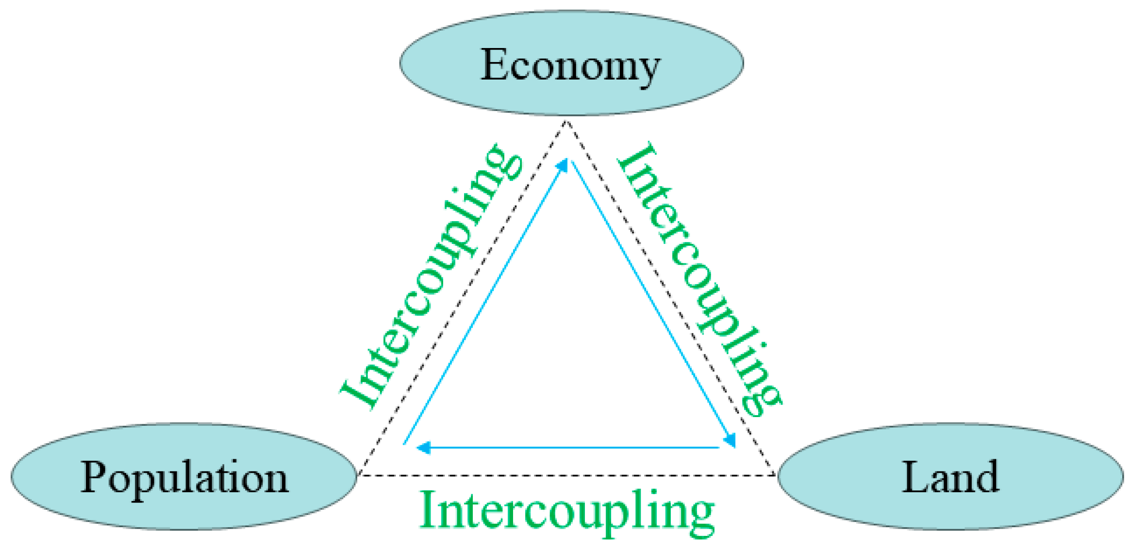
Mabian Yi Autonomous County in Sichuan Province is a typical basin edge mountain area with complex topography. Therefore, this paper takes Mabian Yi Autonomous County of Sichuan Province as the research object and evaluates the geological disasters in this area. Based on the current research results, the information method is used to evaluate the vulnerability of geological disasters in Mabian Yi Autonomous County. At the same time, three models, a support vector machine (SVM), geographically weighted regression (GWR), and multi-layer perceptron (MLP), were constructed to evaluate the hazard of geological disasters in the study area, and the evaluation accuracy of the above three models was compared. Through the two elements of vulnerability evaluation and hazard evaluation, a risk evaluation of geological disasters in the study area was carried out. Finally, the AHP-PCA combination weighting method was used to evaluate the geological environment carrying capacity of the study area. The above research results have great reference basis for the development of economy, population, farming, and animal husbandry and the rational development of geological resources in Mabian Yi Autonomous County. The relationship between the evaluation methods in this paper is shown in Figure 1.

2. Characteristics of Study Area

Mabian Yi Autonomous County is located in the southeast of Leshan City, Sichuan Province, in the mountainous area of southeastern Sichuan on the southern edge of the Sichuan Basin, as shown in Figure 2. As of now, Mabian Yi Autonomous County governs 12 towns and 3 townships. It borders Pingshan County, Yibin City to the east, Liangshan Yi Autonomous Prefecture to the west, and Ebian Yi Autonomous County to the northwest. The coordinates range from 103°14′40″ to 103°49′40″ east longitude, and 28°25′30″ to 29°04′14″ north latitude, with a maximum length of 60.5 km from north to south and a maximum width of 58 km from east to west, with an area of 2304 square kilometers.

The climate of Mabian Yi Autonomous County belongs to the junction of subtropical humid climate and mid-subtropical monsoon climate. The annual average temperature is 15.7 °C. The highest temperature occurs in July with an average of 25.4 °C. The lowest temperature occurs in January with an average of 5.3 °C. Precipitation is abundant, with an average annual precipitation of 976 mm. The main rainy season is from June to September, accounting for more than 70% of the annual precipitation. At the same time, because it is located in a mountainous area, the climate has obvious vertical climate zone characteristics. As the altitude increases, both temperature and precipitation show a decreasing trend. A histogram on precipitation in Mabian Yi Autonomous County from 2000 to 2021 is shown in Figure 3.

In terms of hydrology, Mabian Yi Autonomous County is located in the Minjiang River Basin of the upper reaches of the Yangtze River. There are many rivers in the territory, the water system is developed, and the river density is high. The county is rich in water resources, with an average annual runoff of 10.64 billion cubic meters. However, due to the steep terrain, Mabian Yi Autonomous County has serious soil erosion and poor soil retention capacity. In addition, the climate is relatively arid, and its groundwater resources are relatively scarce.

Mabian Yi Autonomous County is located on multiple fault zones. Most areas in the county are at an altitude of 1000–3500 m. According to statistics from the local emergency management bureau, there are a total of 208 hidden danger points for geological disasters such as debris flows, landslides, and collapses in the study area, as shown in Figure 4 and Figure 5. The main types of geological disasters are landslides and collapses, accounting for 97.6%, including 143 landslides, 60 collapses, and 5 debris flows. See

Table 1. Statistical Table of hidden danger points of geological disasters.

Type	Debris Flow	Landslide	Collapse
Quantity (place)	5	143	60
Proportion	2.40%	68.75%	28.85%

for details. The data of natural conditions such as topography and climate in the above study area are derived from Geospatial Data Cloud [26] and the China Meteorological Administration [27].

3. Methodology

3.1. Data Source

The data used in this study are mainly divided into basic geographic information and remote sensing data. ASTER GDEMV 30M digital elevation data and 30 m global surface coverage data come from geospatial data cloud and GlobeLand30. Water systems data were extracted from digital elevation data. Road data comes from the National Geographic Information Resources Directory Service System; other basic geological data including lithology, geological structure, average annual precipitation, and administrative divisions come from the National Geological Archives and the National Bureau of Statistics.

3.2. Vulnerability Evaluation Method

At present, the evaluation of geological disaster vulnerability has gradually shifted from qualitative evaluation to quantitative evaluation [28]. Among many methods, the information quantity method can quickly and accurately evaluate the information value of each evaluation factor and can be used in different types of comparison between information to quantitatively assess the risk value [29]. This study combines the actual situation of Mabian Yi Autonomous County and uses the information quantity method to evaluate the vulnerability of geological disasters.

3.2.1. Selection of Vulnerability Elements and Their Assessment Factors

The Chinese government takes land finance as the main income, but some ethnic minority areas are sparsely populated, and the economic sources mainly rely on planting, animal husbandry, and tourism. At the same time, the above areas are affected by religious beliefs, which makes the government mainly consider three main factors when implementing governance policies, population, economy, and land resources, which are intercoupled in the above areas (see Figure 6), and it is not comprehensive to discuss them simply from any angle [30,31].

Based on the distribution pattern of geological disasters in Mabian Yi Autonomous County and the basic characteristics of their carriers, this study selected three first-level vulnerability elements: population, economy, and land resources. Among them, population density was used as the population vulnerability evaluation factor, and farmer per capita income was used as the economic vulnerability evaluation factor; the distance from the road, the density of cultivated land, and the density of mineral points were used as land resource vulnerability elements to construct a geological disaster vulnerability evaluation system suitable for Mabian Yi Autonomous County. The details are shown in

Table 2. Vulnerability elements and data sources for evaluating the vulnerability to geological disasters.

Vulnerability Elements	Assessment Factors	Data Sources
Population	Population density	Mabian Yi Autonomous County Statistical Yearbook
Economic	Farmers’ per capita income	Mabian Yi Autonomous County Statistical Yearbook
Land resources	Distance from road	Google Earth remote sensing image
	Plowland density	Landsat-8 remote sensing image
	The density of mineral points	National mineral database

. The grading of each evaluation factor is shown in

Table 3. Grading of vulnerability assessment factors.

Assessment Factors	Grading
Population density	Lower, low, medium, high, higher
Farmers’ per capita income (CNY)	10,000–10,500, 10,500–11,000, 11,000–11,500, 11,500–12,000, >12,000
Distance from road (m)	0–400, 400–800, 800–1200, 1200–1600, >1600
Plowland density	Lower, low, medium, high, higher
The density of mineral points	Low, medium, high
Assessment factors	Grading

.

3.2.2. Evaluation Factor Collinearity Test

Multicollinearity testing can evaluate the correlation between two or more variables [32]. Its role is to help determine the independent variables that can be included in the regression model, as well as the independent variables that need to be eliminated or undergo special treatment; when there is a high degree of correlation between independent variables, the coefficient estimates of the independent variables become unreliable, and overfitting may occur, resulting in poor generalization ability of the model. Therefore, in order to ensure the independence between each evaluation factor, multicollinearity analysis was performed on the selected evaluation factors before evaluating the vulnerability of geological disasters.

Variance influence factor (VIF) and tolerance (TOL) are commonly used multicollinearity testing vulnerability elements, which can be used to evaluate the degree of increase in variance of each independent variable, such as in Equations (1) and (2). Specifically, when VIF > 10 or TOL < 0.1, it indicates that the vulnerability elements have high collinearity.

$$VIF={\displaystyle \frac{1}{1-R{i}^2}}$$

(1)

$$TOL={\displaystyle \frac{1}{VIF}}$$

(2)

Among them, $R_i$ is the coefficient of complex correlation of the ith independent variable with the other independent variables.

This study uses SPSS27 software to conduct multicollinearity analysis on the five selected evaluation factors—population density, per capita income of farmers, distance from roads, cultivated land density, and the density of mineral points—to ensure the accuracy and interpretability of the subsequent model construction. Statistical results of VIF and TOL for each evaluation factor are shown in

Table 4. Co-linearity diagnostics among evaluation factors.

Assessment Factors	VIF	TOL
Population density	2.630	0.380
Farmers’ per capita income	1.983	0.504
Distance from road	3.852	0.259
Plowland density	1.991	0.502
The density of mineral points	2.059	0.486

.

Generally, the smaller the VIF value, the lower the degree of collinearity between the independent variables, and the higher the accuracy and stability of the model. When the VIF value exceeds 10, you need to consider eliminating one or several of the independent variables to reduce the risk of multicollinearity influence. It can be seen from Table 4 that the VIF values of the five selected evaluation factors are all less than 10 and the TOL values are all greater than 0.1. The results meet the requirements of multicollinearity testing, so there is no need to eliminate any evaluation factors.

3.2.3. Information Evaluation Method

The specific calculation steps of the information quantity method are as follows:

(1).

Calculate the geological disaster information value $I\left(X_i,Y\right)$ of each evaluation factor $X_i$, as shown in Equation (3):

$$I\left(X_i,Y\right)=\ln {\displaystyle \frac{\left(N_i/N\right)}{\left(S_i/S\right)}}$$

(3)

Among them, $N_i$ represents the number of geological disaster points in each evaluation factor level, $N$ represents the total number of geological disaster hidden danger points in the study area, $S$ represents the total area of each evaluation factor, and $S_i$ represents the area of each level of each evaluation factor.

(2).

Calculate the total information value of geological disasters for each evaluation factor $I_i$, as shown in Equation (4):

$$I_i=I\left(X_i,Y\right)={\displaystyle \sum _{i=1}^p\ln \frac{\left(N_i/N\right)}{\left(S_i/S\right)}}$$

(4)

Among them, $p$ is the number of selected evaluation factors.

3.3. Hazard Evaluation Method

In recent years, commonly used evaluation methods for geological disaster hazard evaluation have included the analytic hierarchy process, information quantity method, comprehensive fuzzy analysis method, regression model, machine learning model, etc. Each method has different advantages and disadvantages [33]. Fully considering the influence of factors such as topography, geological background, and human engineering activities in Mabian Yi Autonomous County, two machine learning algorithms, support vector machine and multi-layer perceptron, and a multivariate statistical algorithm, namely, geographical weighted regression, were selected to evaluate and analyze the research area. Geological disaster hazard was assessed and compared against the accuracy of the evaluation results of the three methods, and finally the optimal evaluation result of the geological disaster hazard in Mabian Yi Autonomous County was obtained.

During the evaluation process, it is necessary to establish geological disaster hazard evaluation sample points in ArcGIS and use the random generation point tool to randomly generate an equivalent number of non-geological disaster points around the existing 208 geological disaster potential points. The obtained results that can be brought into the data samples of the model (i.e., 208 disaster points and 208 non-disaster sample points) are shown in Figure 7.

3.3.1. Selection and Classification of Hazard Evaluation Factors

The occurrence of geological disasters is the result of complex interactions between multiple influencing factors. Based on the selection principles of geological disaster hazard evaluation factors and the geological environment characteristics of the study area, this study selected topography, geological structures, vegetation coverage, meteorology, hydrology, and human activity. With these five first-level vulnerability elements, we established a geological disaster hazard evaluation system in Mabian Yi Autonomous County, as shown in Figure 8. NDVI is the normalized vegetation index, also known as biomass index change, which is a method used to measure remote sensing to derive an index of the degree of vegetation coverage in the image. The classification of each evaluation factor is shown in

Table 5. The range of the evaluation index interval.

Assessment Factors	Grading
Elevation (m)	499–900, 900–1350, 1350–1800, 1800–2800, >2800
Slope	0–10°, 10–20°, 20–30°, 30–40°, >40°
Slope aspect	East, northeast, southeast, north, south, west, northwest, southwest
RDLS (m)	0–30, 30–75, 75–300, 300–600, >600
Lithology	J2, K1, P1, P2, T1, T2, T3
Geological structure (m)	0–500, 500–1000, 1000–1500, 1500–2000, >2000
NDVI	−0.2–0, 0–0.2, 0.2–0.4, 0.4–0.6, 0.6–0.8, 0.8–1
Mean annual precipitation (mm)	<850, 850–855, 855–860, 860–865, >865
Distance from river (m)	0–300, 300–600, 600–900, 900–1200, >1200
Land use	Artificial surface, woodland, water body, shrubbery, cultivated land, grassland

.

3.3.2. Evaluation Factor Collinearity Test

SPSS software was used to conduct a collinearity test on the selected geological disaster hazard evaluation factors to ensure the independence between each evaluation factor. The test results are shown in

Table 6. Co-linearity diagnostics among evaluation factors.

Assessment Factors	VIF	TOL
Elevation	2.636	0.379
Slope	1.302	0.768
Slope aspect	1.164	0.859
RDLS	1.554	0.644
Lithology	2.985	0.335
Geological structure	1.088	0.919
NDVI	1.167	0.857
Mean annual precipitation	2.414	0.414
Distance from river	1.086	0.921
Land use	1.046	0.956

.

As can be seen from Table 6, the VIF values of the 10 selected geological disaster hazard evaluation factors are all less than 10 and the TOL values are all greater than 0.1, which all meet the multicollinearity test requirements, so no evaluation factors need to be eliminated.

3.3.3. Support Vector Machine Model Construction

Support vector machine (SVM) is a powerful machine learning algorithm commonly used for classification and regression problems [34]. The basic idea of SVM is to map samples to a high-dimensional space so that the samples can be linearly divided in the new space, thereby achieving the purpose of classification [35].

The support vector machine model establishment process is as follows:

(1).

Data processing: Randomly select 80% of the study area hazard evaluation sample data generated in ArcGIS as model training samples, and 20% as model testing samples.

(2).

Determine the hyperplane: On the training set, use the SVM algorithm to determine a hyperplane so that this hyperplane can maximize the margin of different categories of data points. Margin refers to the distance between the hyperplane and the data point closest to it. In order to achieve the objective function (5), the SVM algorithm uses the minimization loss function as an optimization method while satisfying the constraint of interval maximization (6).

$$\mathrm{minsize}:{\displaystyle \frac{1}{2}}\parallel \omega {\parallel }^2$$

(5)

$$y_i({\omega }^T{x}_i+b)\ge 1,(i=1\sim N)$$

(6)

Among them, $\omega$ and $b$ are the linear hyperplane parameters for determining the optimal divisibility, $x_i$ represents the training samples, and $y_i$ represents the type of sample $x_i$. In order to solve the conclusion that minimizing $\parallel \omega {\parallel }^2$ has no solution, it is necessary to introduce slack variables ${\delta }_i$ and penalty coefficients C to the objective function Formula (7), and the slack variables and penalty coefficients constraints are given in Equation (8), which leads to the nonlinear mapping $\phi \left(X_i\right)$.

$$\mathrm{minsize}:{\displaystyle \frac{1}{2}}\parallel \omega {\parallel }^2+C{\displaystyle {\sum }_{i=1}^N{\delta }_i}$$

(7)

$$y_i[{\omega }^T\phi (X_i)+b]\ge 1-{\delta }_i,(i=1\sim N)$$

(8)

(3).

Determine the kernel function: Commonly used kernel functions include the linear kernel function, polynomial kernel function, and Gaussian radial basis kernel function. The radial kernel function (RBF) can map data in low-dimensional space to high-dimensional space, thereby improving the classification accuracy of the model. It has good positive certainty, allowing for the SVM model to be better optimized [36,37]. Therefore, the radial kernel function (Equation (9)) is selected as the kernel function in this support vector machine algorithm.

$$K(x_i, y_j)=e^{{\displaystyle \frac{\parallel x_i-y_i{\parallel }^2}{-{\sigma }^2}}}$$

(9)

In the formula, $\sigma$ represents the width parameter, and the smoothness of the hyperplane of the support vector machine can be optimized by adjusting the $\sigma$ value.

(4).

Hyperparameter optimization: There are some hyperparameters in the SVM algorithm that need to be optimized to obtain the best classification performance. Common hyperparameters include the penalty coefficient C, the width parameter $\sigma$, etc., and the cross-validation technique can usually be used to select the best hyperparameter values. According to the exponentially growing C and γ sequences ($C=2^{-5},2^{-3},\dots ,2^{15},\gamma =2^{-15},2^{-13,}\dots ,2^3$), the parameter C with the highest accuracy rate is finally verified to be 5.021, and the γ is 0.195, which is calculated as Equation (10):

$$\gamma ={\displaystyle \frac{1}{{\sigma }^2}}$$

(10)

(5).

Model evaluation: Use the test set to evaluate the classification performance of the SVM model. At this time, the classification accuracy of the SVM model for the test sample is 85.20%.

3.3.4. Geographically Weighted Regression Model Construction

The specific expression of the geographically weighted regression model is shown Equation (11):

$$y(\mu )={\beta }_0(\mu )+{\displaystyle \sum _{k=1}^p{\beta }_k(\mu )x_k}(\mu )+\epsilon (\mu )$$

(11)

Among them, ${\beta }_0\left(\mu \right)$ represents the intercept, ${\beta }_k\left(\mu \right)$ represents the coefficient of each evaluation factor, $\epsilon \left(\mu \right)$ represents the error.

The core of the geographically weighted regression model is the spatial weight function. The choice of weight function is crucial to the performance and accuracy of the model. Currently, commonly used weight functions include the Gaussian weight function and quadratic weight function. The quadratic weight function has good results when dealing with smooth and non-smooth data but may cause overfitting problems for sparse data; the Gaussian weight function, on the other hand, can model the relationship between distance and weight by means of a Gaussian kernel function, so that weights can be assigned to the relevant data; this method can effectively solve the problem of discontinuous estimates, and can also provide smooth estimates in space [38]. In summary, this study selected the Gaussian weight function based on the nature of the research and the type of data, and its formula is Equation (12).

$$W_{ij}=e^{\left[-{\displaystyle \frac{1}{2}}{\left({\displaystyle \frac{d_{ij}}{r}}\right)}^2\right]}$$

(12)

In the formula, $r$ represents the Gaussian weight function bandwidth, $W$ represents the weighting factor, and $d_{ij}$ represents the distance from observation point j to point i to be measured.

We used the multi-value extraction to point tool in ArcGIS to select the 10 selected evaluation factor values of elevation, slope, aspect, terrain relief, stratum lithology, NDVI, distance from rivers, precipitation, distance from faults, and land use. Geological disaster hazard points and randomly generated sample points were extracted, and a geographically weighted regression model was used to perform geographically weighted regression analysis on all sample points. The coefficients of each evaluation factor are shown in Figure 9. The evaluation factors are superimposed in ArcGIS to finally obtain the geological disaster hazard evaluation results of Mabian Yi Autonomous County.

3.3.5. Multi-Layer Perceptron Model Construction

Multi-layer perceptron (MLP) is a common artificial neural network model with multi-layer nonlinear transformation units and is often used to solve problems such as classification, regression, and pattern recognition [39,40].

This study divided geological disaster hazard point samples and randomly generated sample points into training samples and test samples in a ratio of 7:3, and built a multi-layer perceptron model based on SPSS to combine elevation, slope, aspect, terrain relief, etc. The 10 evaluation factors are set as independent variables, that is, the input layer, and the dependent variable is the geological disaster hazard, that is, the output layer.

The selection of the number of neurons in the hidden layer in the multi-layer perceptron model is very important. It can usually be solved by Equation (13). After continuous calculation and adjustment, it can be concluded that when the number of neurons in the hidden layer is 16, the model verification sample is accurate at the highest rate.

$$N=\sqrt{A+B}+k, (0\le k\le 10)$$

(13)

In the formula, $N$ represents the number of neurons in the hidden layer, $A$ represents the number of neurons in the input layer, $B$ represents the number of neurons in the output layer, $k$ is the empirical coefficient.

In the multi-layer perceptron model, the activation function is a very important component. The function of the activation function is to map the weighted sum of nodes to a certain range to introduce nonlinear properties, thereby improving the expression ability and performance of the model. Common activation functions include the Tanh function, ReLU function, LeakyReLU function, Softmax function, etc. The ReLU function outputs the input value itself in the positive range and outputs 0 in the negative range. It has a simple and efficient calculation method and eliminates gradient disappearance due to the characteristics of the problem [41]—it is widely used. The expression of the ReLU function is given in Equation (14).

$$f(x)=\left\{\begin{array}{c}x, x>0\\ 0, x\le 0\end{array}\right.$$

(14)

The output layer loss function is cross-entropic, and the learning rate init (LRI) was finally determined to be 0.0095 through testing.

3.4. Risk Evaluation Method

The expressions of commonly used disaster risk evaluation models are shown in

Table 7. Risk evaluation model of natural disaster.

Researchers or Institutions	Risk Model Expression
Andrew [42]	Risk = Danger × Vulnerability/Coping capacity
Smith [43]	Risk = Probability × Damage
Stenchion [44]	Risk = Probability + Vulnerability
UNDRO [45]	Risk = Danger × Vulnerability

.

Through comprehensive analysis, the expression of geological disaster risk evaluation function in this paper was determined as follows:

$$\left\{\begin{array}{l}Risk evaluation=f(Hazard evaluation, Carrying capacity evaluation)\\ Vulnerability evaluation=f(Risk evaluation)\end{array}\right.$$

(15)

3.5. Carrying Capacity Evaluation Method

The geological environment carrying capacity refers to the ability of the rocks, soil, hydrogeology, etc., on the Earth’s surface to withstand natural or humanmade factors [46]. It is related to natural disasters, environmental pollution, resource development, etc., and reflects the stability and sustainability in the geological environment. Geological environment carrying capacity evaluation is a process of quantitative or semi-quantitative analysis and evaluation of geological environment carrying capacity. Its purpose is to identify and describe potential geological environmental problems and provide scientific basis for environmental protection and sustainable development.

3.5.1. Selection of Evaluation Indicators for Geological Environment Carrying Capacity

When selecting evaluation factors, the geological environment, social environment, and ecological environment characteristics of Mabian Yi Autonomous County must be fully considered, and the interaction between the geology, ecology, and social environment must be comprehensively considered. Based on the collected data and the actual geological environment of the study area, this study finally selected geological environment: elevation, slope, distance from faults, geological disaster risk; social environment: population density, cultivated land density, distance from roads; ecological environment: eleven evaluation indicators, including average annual precipitation, land use type, distance from rivers, and NDVI, used to construct an evaluation system for the geological environment carrying capacity of Mabian Yi Autonomous County, as shown in Figure 10. The classification of each evaluation index is shown in

Table 8. The range of the evaluation index interval.

Indexes	Grading
Elevation (m)	499–900, 900–1350, 1350–1800, 1800–2800, >2800
Slope	0–10°, 10–20°, 20–30°, 30–40°, 40–50°, 50–60°, >60°
Distance from fault (m)	0–500, 500–1000, 1000–1500, 1500–2000, >2000
Geological disaster risk	Low, medium, high, very high
Population density	Lower, low, medium, high, very high
Plowland density	Lower, low, medium, high, very high
Distance from road (m)	0–400, 400–800, 800–1200, 1200–1600, >1600
Mean annual precipitation (mm)	<850, 850–855, 855–860, 860–865, >865
Land use	Artificial surface, forest land, water body, shrub land, cultivated land, grassland
Distance from river (m)	0–300, 300–600, 600–900, 900–1200, >1200
NDVI	−0.2–0, 0–0.2, 0.2–0.4, 0.4–0.6, 0.6–0.8, 0.8–1

.

3.5.2. AHP-PCA Combination Weighting Method

The combination weighting method is a commonly used comprehensive evaluation method. Its basic idea is to weight a combination of various indicators, comprehensively considering the importance and mutual influence between each indicator, and finally obtain the evaluation results [47].

Based on the principle of combined weighting method, this study uses the analytic hierarchy process (AHP) and principal component analysis (PCA) to combine the subjective and objective weighting methods to assign values to the 11 selected evaluation indicators.

According to the steps of the AHP method, first, the 3 first-level evaluation indicators of geological environment, social environment, and ecological environment were compared in pairs using the 1 to 9 scaling method, and the corresponding judgment matrix was constructed. After calculating the weight vector, we performed a consistency check and calculated the maximum feature vector: ${\lambda }_{\max }=3.104$, $CI=0.052$, $RI=0.58$, $CR=0.089$. The consistency test result was positive. We calculated the weight of the first-level evaluation indicators, and the results are shown in

Table 9. Calculation results of weight for primary evaluation indicators.

Name	1	2	3	Weight
Geological environment	1	5	3	0.637
Social environment	1/5	1	1/3	0.105
Ecological environment	1/3	3	1	0.258

.

Based on the weight calculation results of the first-level evaluation indicators, the weights of the second-level indicators under the geological environment, social environment, and ecological environment indicators were calculated, respectively. The results are shown in

Table 10. Calculation results of weight for geological environment category.

Indexes	1	2	3	4	Weight
Elevation	1	1/2	1/3	1/4	0.122
Slope	2	1	1/2	1/3	0.277
Distance from fault	3	2	1	1/2	0.276
Geological disaster risk	4	3	2	1	0.325

,

Table 11. Calculation results of weight for social environment.

Indexes	1	2	3	Weight
Population density	1	2	4	0.679
Plowland density	1/2	1	2	0.340
Distance from road	1/4	1/2	1	0.080

and

Table 12. Calculation results of weight for ecological environment.

Indexes	1	2	3	4	Weight
Mean annual precipitation	1	1/3	1/2	1	0.148
Land use	3	1	1/3	1/2	0.308
Distance from river	2	2	1	1/3	0.395
NDVI	1	3	2	1	0.148

. Combining the weight results of the first-level evaluation indicators with the second-level indicators under each category, the final weight of each second-level evaluation indicator was calculated, see

Table 13. Calculation results of weight for geological environment category.

Indexes	Geological Environment	Social Environment	Ecological Environment	Final Weight
	0.637	0.105	0.258
Elevation	0.122	0	0	0.078
Slope	0.277	0	0	0.176
Distance from fault	0.276	0	0	0.176
Geological disaster risk	0.325	0	0	0.207
Population density	0	0.679	0	0.071
Plowland density	0	0.340	0	0.034
Distance from road	0	0.080	0	0.008
Mean annual precipitation	0	0	0.148	0.038
Land use	0	0	0.308	0.072
Distance from river	0	0	0.395	0.102
NDVI	0	0	0.148	0.038

.

The general steps for PCA empowerment are as follows:

• Standardize the original data to have a mean of 0 and a variance of 1 for easy processing;
• Based on the standardized data, calculate its covariance matrix;
• Perform eigenvalue decomposition on the covariance matrix to obtain eigenvalues and corresponding eigenvectors;
• According to the size of the eigenvalues, select the largest k eigenvectors as the principal components;
• Multiply the original data by the selected principal component matrix to finally obtain the dimensionally reduced data.

After standardizing the word list data, SPSS was used to construct a principal component matrix, and the objective weights of these 11 evaluation indicators were calculated. In order to comprehensively consider the importance of subjective and objective weights, the calculation coefficient of subjective weights was set to 0.4. The calculation coefficient of the objective weight was set to 0.6. Finally, the two calculation results were superimposed to obtain the combined weight of each evaluation index, as shown in

Table 14. Calculation results of weight for geological environment category.

Indexes	Subjective Weight	Calculation Coefficient	Objective Weight	Calculation Coefficient	Combination Weight
Elevation	0.078	0.4	0.024	0.6	0.0564
Slope	0.176		0.018		0.1128
Distance from fault	0.176		0.022		0.1144
Geological disaster risk	0.207		0.288		0.2394
Population density	0.071		0.148		0.1018
Plowland density	0.034		0.153		0.0816
Distance from road	0.008		0.097		0.0436
Mean annual precipitation	0.038		0.195		0.1008
Land use	0.072		0.019		0.0508
Distance from river	0.102		0.016		0.0676
NDVI	0.038		0.020		0.0308

.

4. Results and Discussion

4.1. Vulnerability Evaluation

According to the calculation steps of the information quantity evaluation method, the information quantity values were calculated for the five selected evaluation factors: population density, per capita income of farmers, distance from roads, cultivated land density, and the density of mineral points. The calculation results are shown in

Table 15. Evaluation factor information value.

Indexes	Grading	Information Magnitude
Population density	Lower	−0.911099
	Low	−0.601309
	Medium	0.175625
	High	0.152425
	Higher	2.292625
Farmers’ per capita income (CNY)	10,000–10,500	−0.423741
	10,500–11,000	−0.162348
	11,000–11,500	−0.160399
	11,500–12,000	0.371094
	>12,000	−0.159291
Distance from road (m)	0–400	0.973748
	400–800	0.910941
	800–1200	0.673695
	1200–1600	0.598538
	>1600	−0.761114
Plowland density	Lower	−1.904801
	Low	0.564881
	Medium	−0.538755
	High	0.712787
	Higher	0.913816
The density of mineral points	Low	−0.123275
	Medium	0.480933
	High	2.306124

.

According to the principle of information quantity model, the higher the information quantity value of an evaluation factor, the greater the probability of geological disasters occurring in the evaluation factor, that is, the evaluation factor is positively correlated with the contribution of geological disaster vulnerability. It can be seen from the calculation results that the evaluation factors with higher information value are classified into high population density range, farmer per capita income in the range of CNY 11,500–12,000, high cultivated land density range, and high mineral point density range.

In ArcGIS, the raster calculator was used to superimpose the information of each evaluation factor to obtain the evaluation results of the vulnerability of geologic disasters in Mabian Yi Autonomous County, and the evaluation results were classified into four grades—low, medium, high, and very high vulnerability—by using the method of natural breakpoints, as shown in Figure 11.

It can be seen from the geological disaster vulnerability zoning map of the study area that Mabian Yi Autonomous County is dominated by highly vulnerable areas, covering an area of approximately 804.12 km², accounting for 33.73% of the area, and is mainly distributed in Suba Town, Sanhekou Town, Xuekoushan Town, and Gaozhuoying Town; the low-vulnerability area covers an area of approximately 782.06 km², accounting for 32.80% of the area, mainly distributed in Qiaoba Town, Dazhubao Town, Yanfeng Town, and Yonghong Town; the medium-vulnerability area is about 372.88 km², accounting for 15.64% of the area, mainly distributed in Meilin Town and Minzhu Town; the very high vulnerability area is about 425.27 km², accounting for 17.84% of the area, mainly distributed in Rongding Town, Xiaxi Town, Minjian Town, Jianshe Town, and areas with dense mining sites in the county.

4.2. Hazard Evaluation

(1).

Support vector machine evaluation model

The test set was used to evaluate the classification performance of the SVM model. Here, the classification accuracy of the SVM model for the test samples is 85.20%.

In ArcGIS, the geological disaster hazard results of the study area calculated by the SVM model were divided into four levels—low hazard, medium hazard, high hazard, and very high hazard—according to the natural breakpoint method, as shown in Figure 12. The area of each dangerous zone and the number of geological disaster hazard points in each zone were calculated through the ArcGIS field calculator. As shown in

Table 16. Geological disaster hazard zoning and density statistics of geological disaster points (SVM).

Hazard Zoning	Area Proportion (%)	Disaster Site Density (Place/km2)
Low	20.62	0.039
Medium	35.46	0.057
High	27.67	0.115
Very high	16.25	0.168

, the area of very high hazard areas accounts for 16.25%, and the density of geological disaster hazard points is 0.168. place/km²; it can be seen that as the geological disaster hazard level increases, the density of geological disaster hidden danger points also gradually increases, which is consistent with the prediction results.

(2).

Geographically weighted regression evaluation model

The above evaluation factors were superimposed in ArcGIS to finally obtain the geological disaster hazard evaluation results of Mabian Yi Autonomous County, and the natural breakpoint method was used to divide them into low hazard, medium hazard, high hazard, and very high hazard, as shown in Figure 13. The area of each dangerous zone and the number of geological disaster hazard points in each zone were calculated through the ArcGIS field calculator, see

Table 17. Geological disaster hazard zoning and density statistics of geological disaster points (GWR).

Hazard Area	Area Proportion (%)	Disaster Site Density (Place/km2)
Low	5.77	0.091
Medium	18.75	0.074
High	47.60	0.080
Very high	27.88	0.105

; the very high-hazard areas account for 27.88%, and the density of geological disaster points is 0.105 place/km²; the proportion of high-hazard areas is 47.60%, and the density of geological disaster points is 0.080 place/km²; the area proportion of medium-hazard areas is 18.75%, and the density of geological disaster points is 0.074 place/km²; the area proportion of low-hazard areas is 5.77%, and the density of geological disaster points is 0.091 place/km². It can be clearly seen that as the geological disaster hazard level increases, the density of geological disaster points also gradually increases, which is consistent with the prediction results.

(3).

Multi-layer perceptron model construction

After continuous iterative calculations, the trained model was obtained and used to predict test samples. The prediction accuracy of the multi-layer perceptron model was 87.5%. In ArcGIS, the geological disaster hazard results of the study area evaluated by the multi-layer perceptron model were divided into four levels—low hazard, medium hazard, high hazard, and very high hazard—using the natural breakpoint method, as shown in Figure 14.

We used the ArcGIS field calculator to calculate the area of each dangerous zone and the number of geological disaster points in each zone. As shown in

Table 18. Geological disaster hazard zoning and density statistics of geological disaster points (MLP).

Hazard Zoning	Area Proportion (%)	Disaster Site Density (Place/km2)
Low	16.03	0.032
Medium	30.00	0.051
High	35.87	0.065
Very high	18.10	0.246

, the area of low-hazard areas accounts for 16.03%, the area of medium-hazard areas accounts for 30.00%, and the area of high-hazard areas the proportion is 35.87%, and the area of very high-hazard areas accounts for 18.10%. Among them, the density of geological disaster points in very high-hazard areas is the highest, 0.246 place/km². It can be clearly seen that as the hazard level increases, the number of disaster points increases. The distribution density gradually increases, and the predicted results can be obtained, consistent with the actual situation.

(4).

Comparison of model evaluation results

In terms of area, the area proportion of very high-hazard areas in the SVM model evaluation results is 16.25%, the area proportion of very high-hazard areas in the GWR model evaluation results is 27.88%, and the area proportion of very high-hazard areas in the MLP model evaluation results is 18.10%. Among them, the very high-hazard area is the largest in the GWR model evaluation results, and the very high-hazard area is the smallest in the SVM model evaluation results. In the SVM model evaluation results, the elevation factor has a significant impact on the geological disaster hazard of the study area. The GWR model in the evaluation results, the factors of elevation, and distance from the river have a greater impact on the hazard of geological disasters in the study area. In the evaluation results of the MLP model, the factor of distance from the river has a more prominent impact on the hazard of geological disasters in the study area. Therefore, the evaluation results of the SVM and MLP models’ medium- and very high-hazard areas are scattered, while GWR is relatively more concentrated. For the density of geological disaster points in very high-hazard areas, the MLP model evaluation result is the largest, and the GWR model evaluation result is the smallest.

In order to quantitatively evaluate the performance of the model, this study uses the ROC curve for evaluation, which is the receiver operating characteristic curve, a tool often used to evaluate the performance of classifiers [48]. The advantage is that it is not affected by the imbalance of positive and negative samples. In practical applications, the ratio of positive and negative samples may be very different, and the ROC curve can show the performance of the classifier under different category ratios. It is affected by changes in the ratio of positive and negative samples and can provide an intuitive trade-off solution. The AUC (area under the curve) value in the ROC curve refers to the area under the ROC curve, and its value range is between 0.0 and 1.0. Specifically, the higher the AUC value, the better the accuracy of the model. Therefore, the ROC curve was used to test the accuracy of the SVM, GWR, and MLP models for the geological disaster hazard evaluation results in the study area, as shown in Figure 15. The AUC value of the SVM model is 0.852, the AUC value of the GWR model is 0.911, and for the MLP model, the AUC value is 0.857. The results show that the geographically weighted regression model has the highest value AUC, which means that the geographically weighted model is the most accurate in assessing geological disaster hazard in the study area.

4.3. Risk Evaluation

In this study, Equation (15) was used to calculate and evaluate the risk of Mabian Yi Autonomous County. The vulnerability evaluation results calculated by the information volume model and the geographically weighted regression model were used in ArcGIS. The risk evaluation results were multiplied by raster operations to finally obtain the geological disaster risk evaluation results of the study area. The natural breakpoint method was used to divide the geological disaster risk evaluation results into low risk, medium risk, high risk and very high risk, as shown in Figure 16.

Using ArcGIS field calculator statistical analysis, it can be clearly seen that the very high-risk areas in Mabian Yi Autonomous County cover an area of 564.88 km², accounting for 23.90%, and are mainly distributed in Xiaxi Town, Sanhekou Town, Jianshe Town, Minjian Town, Rongding Town, the northeastern part of Suba Town, and Yanfeng Town, areas where mineral points are densely distributed.

The high-risk areas cover 909.29 km², accounting for 38.47%, and are mainly distributed in Meilin Town, southern Suba Town, and western Minzhu Town.

The medium-risk areas cover an area of 637.52 km², accounting for 26.97%, and are mainly distributed in the northern part of Dazhubao Township, Yonghong Township, and the western part of Yanfeng Town, with a few remaining areas in the northeastern part of Minzhu Town.

The low-risk areas cover an area of 251.89 km², accounting for 10.66%, and are mainly distributed in Qiaoba Town, eastern Yonghong Town, and southern Dazhubao. Statistics on the distribution of geological disaster points in areas with various risk levels are shown in

Table 19. Statistical table of risk zonation of geological disasters.

Risk Zoning	Area Proportion (%)	Disaster Site Density (Place/km2)
Low	10.66	0.0437
Medium	26.97	0.0753
High	38.47	0.0968
Very high	23.90	0.1079

. It can be seen that the density of geological disaster points in very high-risk areas is the highest, at 0.1079 place/km².

4.4. Carrying Capacity Evaluation

ArcGIS tools were used to superimpose the 11 factor weights, and finally the geological environment carrying capacity evaluation results of Mabian Yi Autonomous County were obtained. The natural breakpoint method was used to divide the geological environment carrying capacity results into four levels: low carrying capacity, medium carrying capacity, high carrying capacity, and very high carrying capacity, as shown in Figure 17.

We statistically analyzed the area of each bearing capacity level and the distribution of geological disaster points in areas with different bearing capacity levels, as shown in

Table 20. Statistical analysis of geological environment carrying capacity zoning in study area.

Geological Environment Carrying Capacity Level	Area Proportion (%)	Disaster Site Density (Place/km2)
Low	23.74	0.1565
Medium	25.66	0.0559
High	13.66	0.1391
Very high	36.94	0.0469

. The very high carrying capacity area is 875.04 km², accounting for 36.94% of the area, and is mainly distributed in Dazhubao Township, Qiaoba Town, Yonghong Township, and the western part of Yanfeng Town.

The area of high bearing capacity is 323.61 km², accounting for 13.66% of the area, and the density of local disaster points is 0.1391 place/km². It is mainly distributed in the west of Minzhu Town, the east of Suba Town, and a few in the south of Xuekoushan Town.

The area with medium carrying capacity is 607.68 km², accounting for 25.66% of the area, and the density of disaster points is 0.0559 place/km² It is mainly distributed in Meilin Town, the east of Laodong Town, the boundary of Sanhekou Town, and the northwest of Minzhu Town.

The area of low bearing capacity is 562.27 km², accounting for 23.74% of the area. The density of geological disaster points is 0.1565 place/km². It is mainly distributed in Xiaxi Town and Rongding Town. Minjian Town, Jianshe Town, and Yanfeng Town have a higher mineral density; the central part of Sanhekou Town also covers a wide area.

5. Conclusions

This article conducted research on the vulnerability, hazard, risk, and geological environment carrying capacity of geological disasters in Mabian Yi Autonomous County, Sichuan, a mountainous area. The specific conclusions are as follows:

• The study area is dominated by high-vulnerability areas, and through comparison, it was found that the evaluation results of the geographically weighted regression model are more accurate. The evaluation results of the environmental carrying capacity of geological disasters in Mabian Yi Autonomous County were obtained by calculation. The area of very high carrying capacity is 875.04 km², accounting for 36.94%, mainly distributed in Dazhubao Township, Qiaoba Town, Yonghong Township, and the west of Yanfeng Town. The area of high carrying capacity is 323.61 km², accounting for 13.66%. It is mainly distributed in the west of Minzhu Town and the east of Suba Town, and a little in the south of Xuekoushan Town. The area of medium carrying capacity is 607.68 km², accounting for 25.66% of the total area. It is mainly distributed in the eastern part of Meilin Town, Laodong Town, the boundary of Sanhekou Town, and the northwest of Minzhu Town. The area of low carrying capacity is 562.27 km², accounting for 23.74%. It is mainly distributed in Xiaxi Town, Rongding Town, Minjian Town, Jianshe Town, Yanfeng Town, and the middle of Sanhekou Town;
• The hazard of geological disasters in Dazhubao Town, Xuekoushan Town, Minjian Town, Jianshe Town, Suba Town, Qiaoba Town, and Minzhu Town is low. Therefore, in order to reduce the threat of natural disasters, the abovementioned areas can be considered as population concentration areas, meaning that the population in high-hazard areas and very high-hazard areas of geological disasters need to be relocated;
• When considering the development plan of economic construction, low-hazard areas such as Sanhekou Town, Meilin Town, Yanfeng Town, Gaozhuoying Township, Yonghong Township, Xiaxi Town, Rongding Town, and Laodong Town can be used as nature reserves to rationally develop animal husbandry and reduce mining. Dazhubao Town, Xuekoushan Town, Minjian Town, Jianshe Town, Suba Town, Qiaoba Town, and Minzhu Town can reasonably develop modern agriculture and tourism;
• The concentration of population and the development of tourism will inevitably increase the vulnerability and risk of geological disasters in related areas. Therefore, it is necessary to strengthen the infrastructure in Dazhubao Township, Xuekoushan Town, Minjian Town, Jianshe Town, Suba Town, Qiaoba Town, and Minzhu Town, so as to enhance the ability of the above areas to resist geological disasters via dam reinforcement, house reinforcement, strengthening drainage facilities, etc. At the same time, the construction of the monitoring, early warning, and forecasting systems should be strengthened to improve the early detection of geological disasters. It is suggested to carry out social publicity and education activities to strengthen the public’s self-disaster prevention awareness and coping ability, and to strictly limit the development and utilization of, as well as reduce the impact of human activities on, the natural environment;
• There are still many shortcomings in this study. This paper does not carry out a detailed analysis of a single factor and establish a mathematical model, and there are not enough observation samples to verify the correctness of the inference. Therefore, in a follow-up study, we will continue to monitor the changes in geological disasters in the study area, making the disaster management research in Mabian Yi Autonomous County more and more perfect.

References

1. Wang, H.F.; Cao, H.L.; Kai, Y.; Bai, H.C.; Chen, X.F.; Yang, Y.; Xing, L.; Zhou, C.J. Multi-Source Remote Sensing Intelligent Characterization Technique-Based Disaster Regions Detection in High-Altitude Mountain Forest Areas. IEEE Geosci. Remote Sens. Lett. 2022, 19, 3512905. [Google Scholar] [CrossRef]
2. Yong, Y.; Xin, G.; Zhang, S.C. Multimedia based risk forecasting model for frequent natural disasters. Multimed. Tools Appl. 2020, 79, 35463–35474. [Google Scholar] [CrossRef]
3. Cao, F.F.; Wang, H.Y.; Zhang, C.L.; Kong, W.B. Social Vulnerability Evaluation of Natural Disasters and Its Spatiotemporal Evolution in Zhejiang Province, China. Sustainability 2023, 15, 6400. [Google Scholar] [CrossRef]
4. Yang, J.M.; Hou, H.P.; Hu, H.Q. Exploring the Intelligent Emergency Management Mode of Rural Natural Disasters in the Era of Digital Technology. Sustainability 2024, 16, 2366. [Google Scholar] [CrossRef]
5. Poo, M.M. Innovation and reform: China’s 14th Five-Year Plan unfolds. Natl. Sci. Rev. 2021, 8, nwaa294. [Google Scholar] [CrossRef] [PubMed]
6. Hou, J.; Lv, J.; Chen, X.; Yu, S. China’s regional social vulnerability to geological disasters: Evaluation and spatial characteristics analysis. Nat. Hazards 2016, 84, S97–S111. [Google Scholar] [CrossRef]
7. He, Z.; Yu, M.; Li, J. Evaluation of geological hazard susceptibility in loess disaster area based on gis technology. Fresenius Environ. Bull. 2022, 31, 10708–10715. [Google Scholar]
8. Wang, T.; Zhou, D.; Wang, L.; Wu, J. Urban Spatial Carrying Capacity and Sustainable Urbanization in the Middle-east Section of North Slope of Kunlun Mountains in Xinjiang, China. Chin. Geogr. Sci. 2023, 33, 426–440. [Google Scholar] [CrossRef]
9. Wu, X.; Hu, F. Analysis of ecological carrying capacity using a fuzzy comprehensive evaluation method. Ecol. Indic. 2020, 113, 106243. [Google Scholar] [CrossRef]
10. Carrara, A. A multivariate model for landslide hazard evaluation. J. Int. Assoc. Math. Geol. 1983, 15, 403–426. [Google Scholar] [CrossRef]
11. Brabb, E.E. Innovative approaches to landslide hazard mapping. In Proceedings of the 4th International Symposium on Landslides, Toronto, ON, Canada, 16–21 September 1984; pp. 307–324. [Google Scholar]
12. Carrara, A.; Cardinali, M.; Detti, R.; Guzzetti, F.; Pasqui, V.; Reichenbach, P. GIS techniques and statistical models in evaluating landslide hazard. Earth Surf. Process. Landf. 1991, 16, 427–445. [Google Scholar] [CrossRef]
13. Gupta, R.P.; Joshi, B.C. Landslide Hazard Zoning Using the GIS Approach—A case Study from the Ramganga Catchment, Himalayas. Eng. Geol. 1990, 28, 119–131. [Google Scholar] [CrossRef]
14. Lee, S.; Pradhan, B. Landslide hazard mapping at Selangor, Malaysia using frequency ratio and logistic regression models. Landslides 2007, 4, 33–41. [Google Scholar] [CrossRef]
15. Varnes, D.J. Landslide hazard zonation: A review of principles and practice. Nat. Hazards 1984, 3, 63. [Google Scholar] [CrossRef]
16. Niu, Q.; Cheng, W.; Liu, Y.; Xie, Y.; Lan, H.; Cao, Y. Risk assessment of secondary geological disasters induced by the Yushu earthquake. J. Mt. Sci. 2012, 9, 232–242. [Google Scholar] [CrossRef]
17. Hearn, G.J. Landslide and erosion hazard mapping of Ok Tedi copper mine, Papua New Guinea. Q. J. Eng. Geol. 1995, 28, 47–60. [Google Scholar] [CrossRef]
18. Xu, F.-g.; Ou, Y.-h.; Wang, F.; Wei, B.-w.; Ruokun, N. Risk assessment of geological disasters in Beichuan County after the Wenchuan earthquake based on ArcGIS. Bull. Eng. Geol. Environ. 2023, 82, 416. [Google Scholar] [CrossRef]
19. Anbalagan, R.; Singh, B. Landslide hazard and risk assessment mapping of mountainous terrains—A case study from Kumaun Himalaya, India. Eng. Geol. 1996, 43, 237–246. [Google Scholar] [CrossRef]
20. Chang, M.; Dou, X.; Tang, L.; Xu, H. Risk assessment of multi-disaster in Mining Area of Guizhou, China. Int. J. Disaster Risk Reduct. 2022, 78, 103128. [Google Scholar] [CrossRef]
21. William, R.D. Systems Agriculture: Inquiry and Action for Global Applications: Proceedings of a symposium sponsored by The International Affairs Committee of the Weed Science Society of America February 7, 1991, Louisville, Kentucky. Weed Technol. 1992, 6, 451. [Google Scholar] [CrossRef]
22. Vartanyan, G.S.; Kurennoy, V.; Sychev, K. Regional cooperation of the european socialist countries in developing the fundamentals for an automated system of groundwater assessment. IAHS-AISH Publ. 1990, 173, 93–97. [Google Scholar]
23. Arrow, K.; Bolin, B.; Costanza, R.; Dasgupta, P.; Folke, C.; Holling, C.S.; Jansson, B.O.; Levin, S.; Maler, K.G.; Perrings, C.; et al. Economic growth, carrying capacity, and the environment. Science 1995, 268, 520–521. [Google Scholar] [CrossRef] [PubMed]
24. Witten, J.D. Carrying Capacity and the Comprehensive Plan: Establishing and Defending Limits to Growth. Boston Coll. Environ. Aff. Law Rev. 2001, 28, 147–156. [Google Scholar]
25. McKeon, G.M.; Stone, G.S.; Syktus, J.I.; Carter, J.O.; Flood, N.R.; Ahrens, D.G.; Bruget, D.N.; Chilcott, C.R.; Cobon, D.H.; Cowley, R.A.; et al. Climate change impacts on northern Australian rangeland livestock carrying capacity: A review of issues. Rangel. J. 2009, 31, 1–29. [Google Scholar] [CrossRef]
26. Geospatial Data Cloud. Available online: https://www.gscloud.cn/ (accessed on 24 July 2024).
27. China Meteorological Administration. Available online: https://weather.cma.cn/ (accessed on 24 July 2024).
28. Li, M.; Lv, J.; Chen, X.; Jiang, N. Provincial evaluation of vulnerability to geological disaster in China and its influencing factors: A three-stage DEA-based analysis. Nat. Hazards 2015, 79, 1649–1662. [Google Scholar] [CrossRef]
29. Xiong, J.; Wu, J. Construction of information network vulnerability threat assessment model for CPS risk assessment. Comput. Commun. 2020, 155, 197–204. [Google Scholar] [CrossRef]
30. Chen, L.; Yu, L.S.; Yin, J.B.; Xi, M.J. Impact of Population Density on Spatial Differences in the Economic Growth of Urban Agglomerations: The Case of Guanzhong Plain Urban Agglomeration, China. Sustainability 2023, 15, 14601. [Google Scholar] [CrossRef]
31. Zhang, X.; Luo, H.; Zeng, X.Y.; Zhou, C.Y.; Shu, Z.L.; Li, H.Y.; Fei, Z.; Liu, G.C. Research on regional economic development and natural disaster risk assessment under the goal of carbon peak and carbon neutrality: A case study in Chengdu-Chongqing economic circle. Land Use Policy 2024, 143, 107206. [Google Scholar] [CrossRef]
32. Graham, M.H. Confronting multicollinearity in ecological multiple regression. Ecology 2003, 84, 2809–2815. [Google Scholar] [CrossRef]
33. Shao, M.; Hou, S.; Gao, J. Using the Information Quantity Method to Assess the Regional Risk of Highway Slope to Improve the Level of Risk Management. Adv. Civ. Eng. 2023, 2023, 9118355. [Google Scholar] [CrossRef]
34. Jain, S.; Rastogi, R. Parametric non-parallel support vector machines for pattern classification. Mach. Learn. 2022, 113, 1567–1594. [Google Scholar] [CrossRef]
35. Ramirez-Morales, A.; Salmon-Gamboa, J.U.; Li, J.; Sanchez-Reyna, A.G.; Palli-Valappil, A. Boosted support vector machines with genetic selection. Appl. Intell. 2023, 53, 4996–5012. [Google Scholar] [CrossRef]
36. Almaiah, M.A.; Almomani, O.; Alsaaidah, A.; Al-Otaibi, S.; Bani-Hani, N.; Al Hwaitat, A.K.; Al-Zahrani, A.; Lutfi, A.; Awad, A.B.; Aldhyani, T.H.H. Performance Investigation of Principal Component Analysis for Intrusion Detection System Using Different Support Vector Machine Kernels. Electronics 2022, 11, 3571. [Google Scholar] [CrossRef]
37. Yalsavar, M.; Karimaghaee, P.; Sheikh-Akbari, A.; Khooban, M.-H.; Dehmeshki, J.; Al-Majeed, S. Kernel Parameter Optimization for Support Vector Machine Based on Sliding Mode Control. IEEE Access 2022, 10, 17003–17017. [Google Scholar] [CrossRef]
38. Mardalena, S.; Purhadi, P.; Purnomo, J.D.T.; Prastyo, D.D. The Geographically Weighted Multivariate Poisson Inverse Gaussian Regression Model and Its Applications. Appl. Sci. 2022, 12, 4199. [Google Scholar] [CrossRef]
39. Moustafa, E.B.; Elsheikh, A. Predicting Characteristics of Dissimilar Laser Welded Polymeric Joints Using a Multi-Layer Perceptrons Model Coupled with Archimedes Optimizer. Polymers 2023, 15, 233. [Google Scholar] [CrossRef]
40. Shahriyari, M.; Safari, A.; Quteishat, A.; Afsharirad, H. A short-term voltage stability online assessment based on multi-layer perceptron learning. Electr. Power Syst. Res. 2023, 223, 109562. [Google Scholar] [CrossRef]
41. Krizhevsky, A.; Sutskever, I.; Hinton, G. ImageNet Classification with Deep Convolutional Neural Networks. Commun. ACM 2017, 60, 84–90. [Google Scholar] [CrossRef]
42. Andrew, M. Disaster Mitigation: A Community Based Approach; Oxfam GB: Oxford, UK, 1989; pp. 1–100. [Google Scholar]
43. Smith, K. Environmental Hazard—Assessing Risk and Reducing Disaster. Geogr. J. 1997, 159, 349. [Google Scholar] [CrossRef]
44. Stenchion, P. Development and disaster management. Aust. J. Emerg. Manag. 1997, 12, 40–44. [Google Scholar] [CrossRef]
45. UNDRO. Mitigating Natural Disasters Phenomena Effects and Options a Manual for Policy Makers and Planners; UNDRO: New York, NY, USA, 1991. [Google Scholar]
46. Wang, Z.; He, X.; Zhang, C.; Xu, J.; Wang, Y. Evaluation of Geological and Ecological Bearing Capacity and Spatial Pattern along Du-Wen Road Based on the Analytic Hierarchy Process (AHP) and the Technique for Order of Preference by Similarity to an Ideal Solution (TOPSIS) Method. Isprs Int. J. Geo-Inf. 2020, 9, 237. [Google Scholar] [CrossRef]
47. Zhou, J.-L.; Xu, Q.-Q.; Zhang, X.-Y. Water Resources and Sustainability Assessment Based on Group AHP-PCA Method: A Case Study in the Jinsha River Basin. Water 2018, 10, 1880. [Google Scholar] [CrossRef]
48. Jiang, W.; Rao, P.; Cao, R.; Tang, Z.; Chen, K. Comparative evaluation of geological disaster susceptibility using multi-regression methods and spatial accuracy validation. J. Geogr. Sci. 2017, 27, 439–462. [Google Scholar] [CrossRef]
Figure 1. Research idea.
Sustainability 16 07170 g001
Figure 2. Geographical location of the study area.
Sustainability 16 07170 g002
Figure 3. Distribution of rainfall in Mabian Yi Autonomous County for the period 2000–2021.
Sustainability 16 07170 g003
Figure 4. Distribution of hidden geological disaster points in study area.
Sustainability 16 07170 g004
Figure 5. Hidden danger points of geological disasters in Mabian Yi Autonomous County.
Sustainability 16 07170 g005
Figure 6. The relationship between population, economy, and land resources.
Sustainability 16 07170 g006
Figure 7. Sample data of geological disaster hazard evaluation in study area.
Sustainability 16 07170 g007
Figure 8. Geological disaster hazard evaluation index system in study area (relief degree of land Surface, RDLS).
Sustainability 16 07170 g008
Figure 9. (a) Coefficients of NDVI; (b) coefficients of slope gradient; (c) coefficients of elevation; (d) coefficients of altitude; (e) coefficients of lithology; (f) coefficients of appearance; (g) coefficients of land use type; (h) coefficients of river distance; (i) coefficients of fault distance; (j) coefficients of annual rainfall.
Sustainability 16 07170 g009
Figure 10. Geological environment carrying capacity evaluation index system in study area.
Sustainability 16 07170 g010
Figure 11. Geological disaster vulnerability zonation map.
Sustainability 16 07170 g011
Figure 12. Geological disaster hazard evaluation zoning map (SVM).
Sustainability 16 07170 g012
Figure 13. Geological disaster hazard evaluation zoning map (GWR).
Sustainability 16 07170 g013
Figure 14. Geological disaster hazard evaluation zoning map (MLP).
Sustainability 16 07170 g014
Figure 15. Receiver operating characteristic curve of three models (Invalid curve: Represents the result of random guessing, and the lower part of the invalid curve indicates that the model has no recognition ability).
Sustainability 16 07170 g015
Figure 16. Geological disaster risk zoning map.
Sustainability 16 07170 g016
Figure 17. Zoning map for geological environment carrying capacity.
Sustainability 16 07170 g017