Understanding the Relationship between Urban Form and Urban Shrinkage among Medium-Sized Cities in Poland and Its Implications for Sustainability


Abstract
1. Introduction
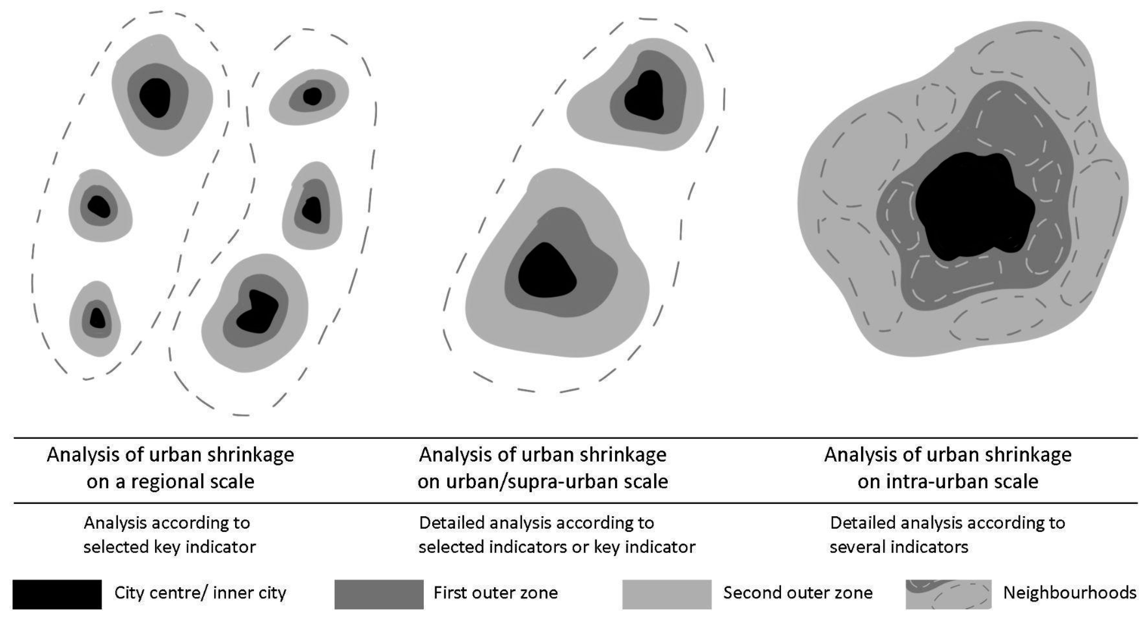
2. Spatial Patterns of Urban Shrinkage
2.1. State of Research on Spatial Patterns of Urban Shrinkage
2.1.1. Regional or Inter-Urban Scale
2.1.2. Urban and Supra-Urban Scale
2.1.3. Intra-Urban Scale
2.2. Polish Urban Shrinkage Context
2.3. Compactness
3. Materials and Methods
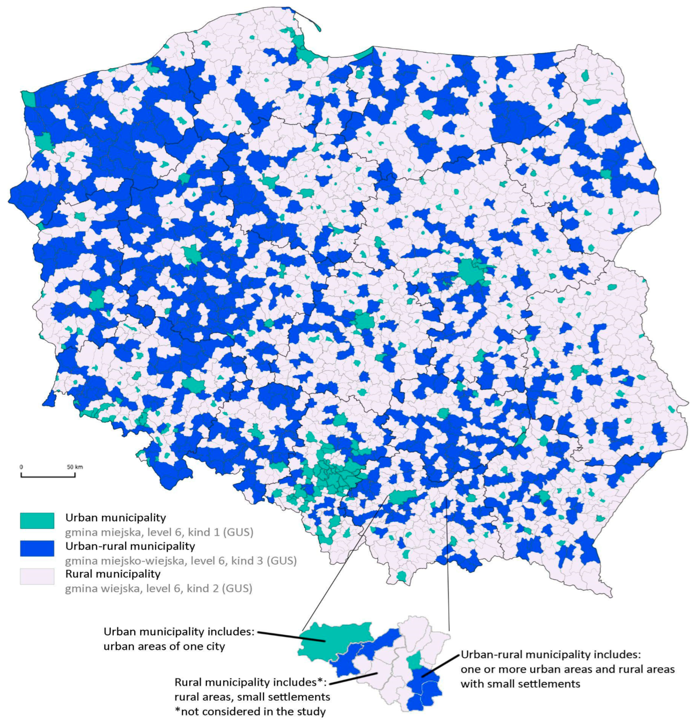
3.1. Subjects
- -
- urban area in the urban municipality (6, 1),
- -
- an urban area in the urban-rural municipality (6, 3), including a city and small settlements.
3.2. Timeframe
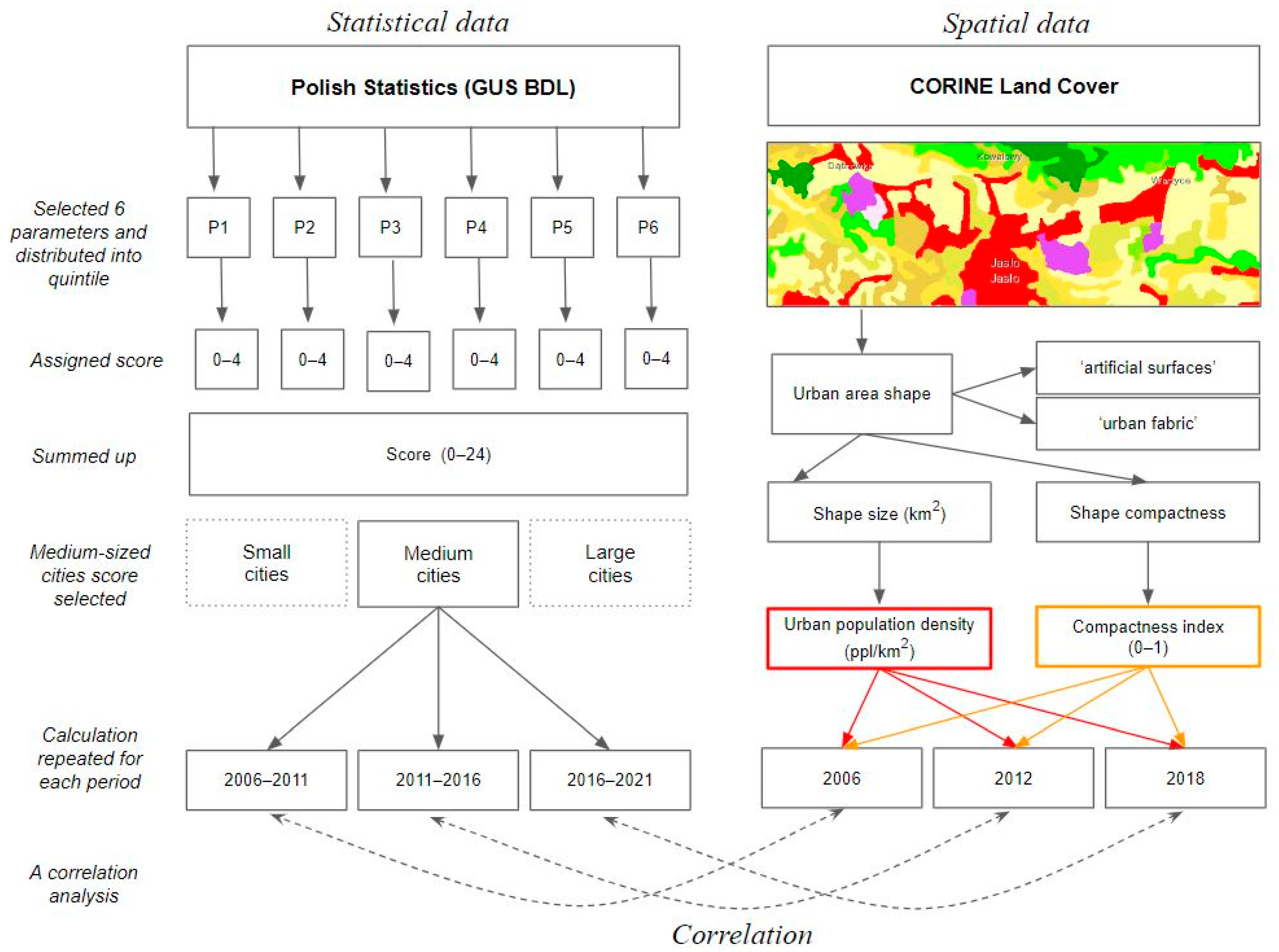
3.3. Statistical Data
3.4. Spatial Data
- Artificial surfaces—built-up areas, including residential areas, commercial and industrial areas, mines, and green urban spaces.
- Agricultural areas—arable land, permanent crops, meadows, pastures, and land principally occupied by agriculture with significant areas of natural vegetation.
- Forests and semi-natural areas—forests, shrubs, and open areas with little or no vegetation.
- Wetlands—inland marshes, peat bogs, salt marshes, salines, and intertidal flats.
- Water bodies—inland waters and marine waters.
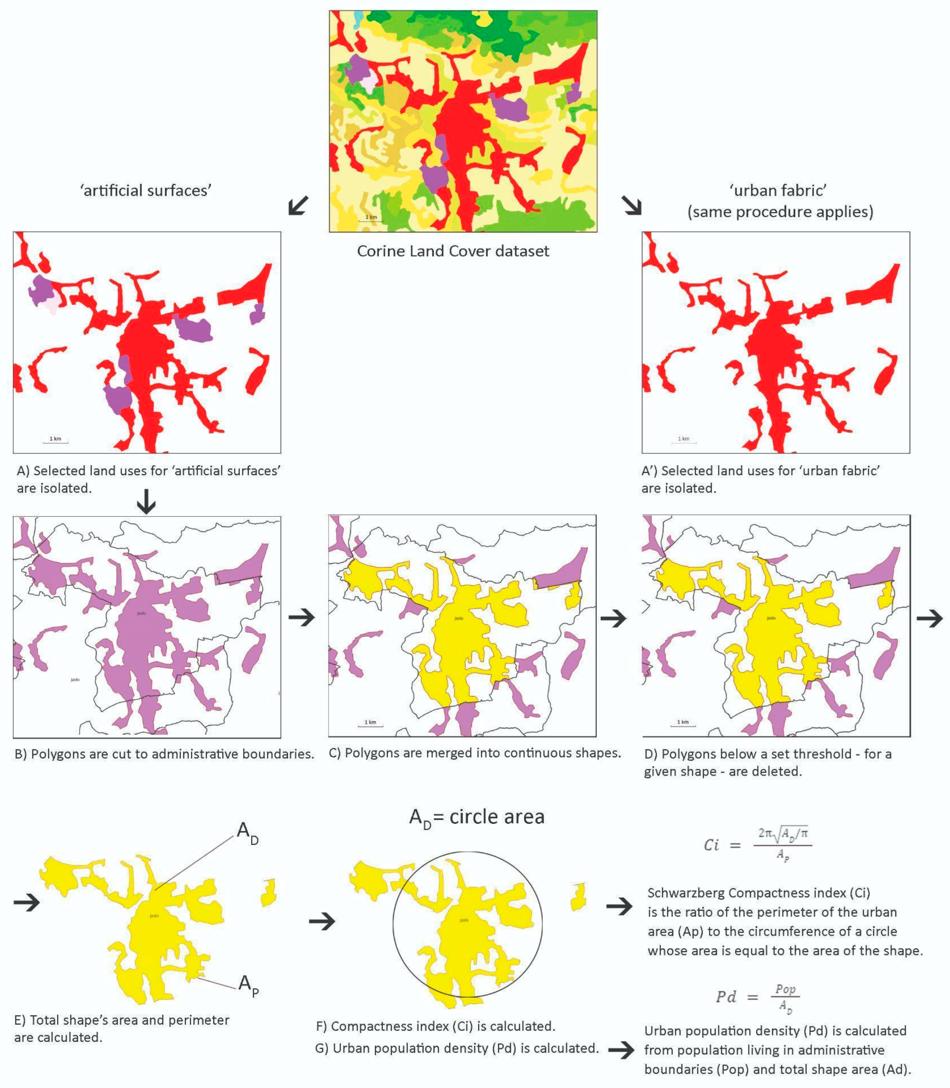
3.5. Defining Urban Compactness
- Isolation of selected land use classes;
- A cut of land-use polygons with city administrative boundaries;
- Merge polygons into continuous shapes;
- Delete polygons below a set threshold for a particular shape;
- Calculate the shape’s area and perimeter;
- Calculate the compactness index;
- Calculate the urban population density.
3.5.1. Spatial Measures
| AD | Urban area |
| AP | Urban area perimeter length |
| Ci | Compactness index |
| Pop | Urban population |
| Pd | Urban population density |
Compactness Index Calculation
Urban Population Density Calculation
3.5.2. Statistical Correlation Analysis between Spatial Measures and Urban Shrinkage
3.6. Tools
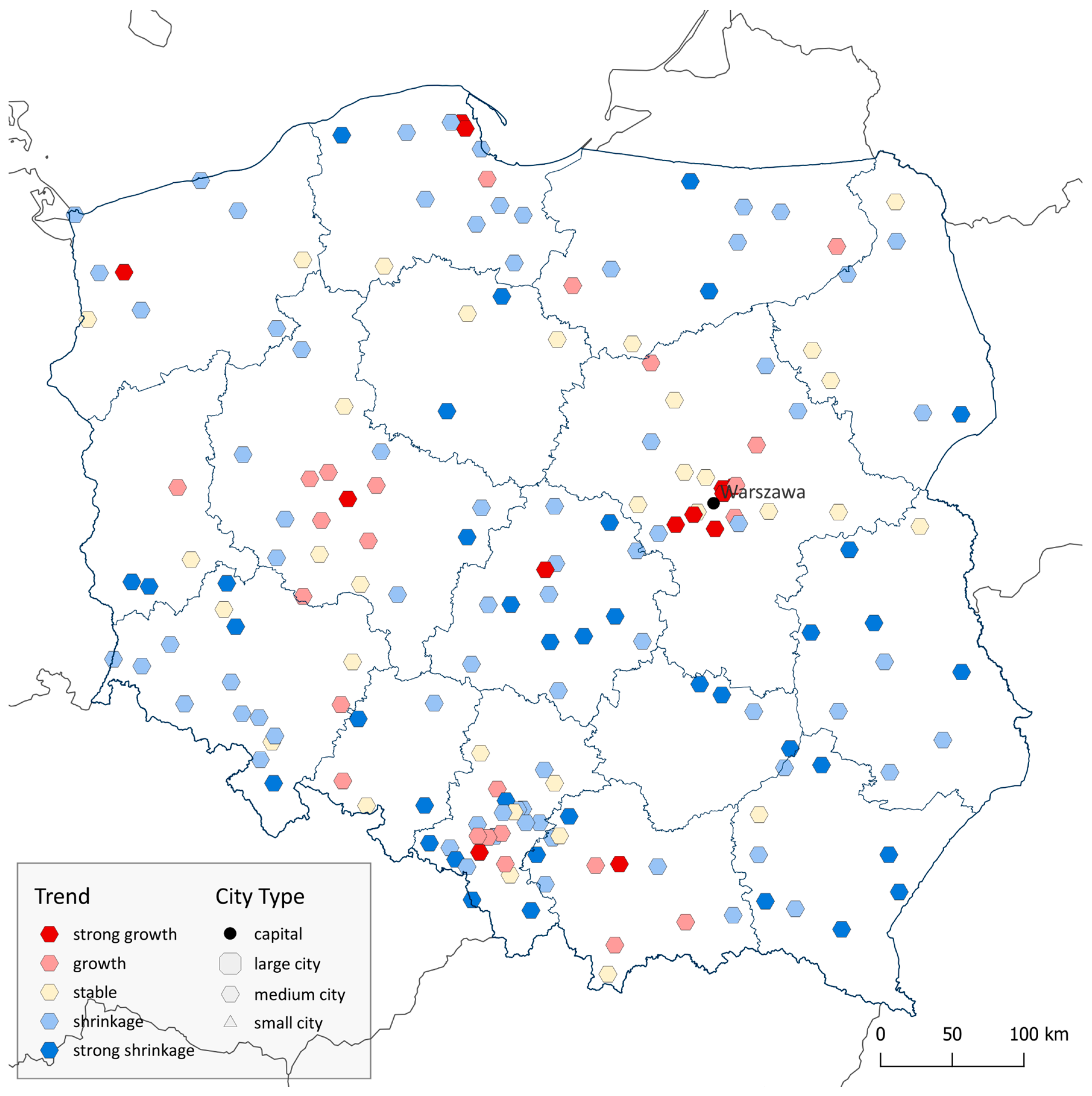
4. Results
4.1. Spatial Measures Calculation Outcomes
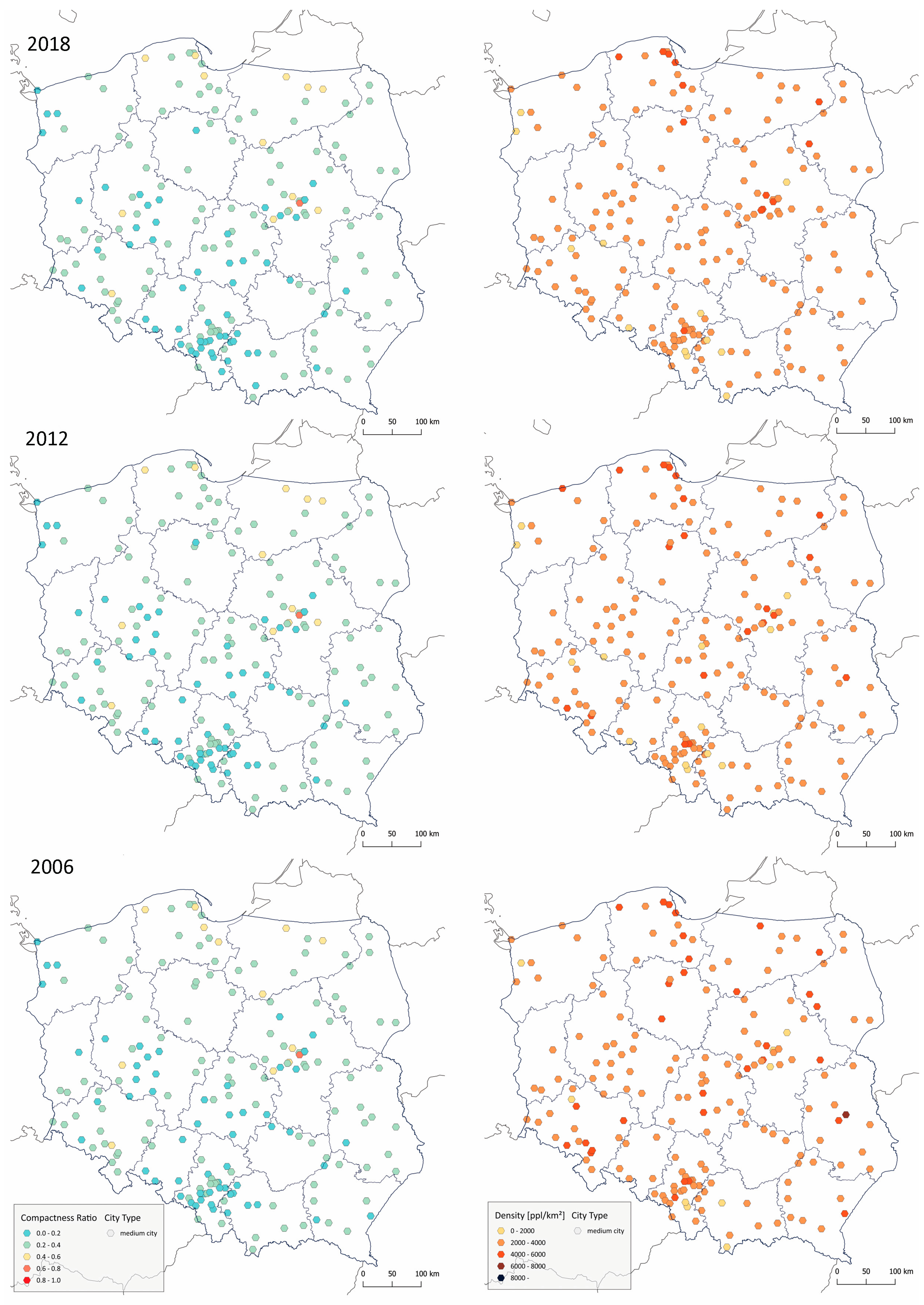
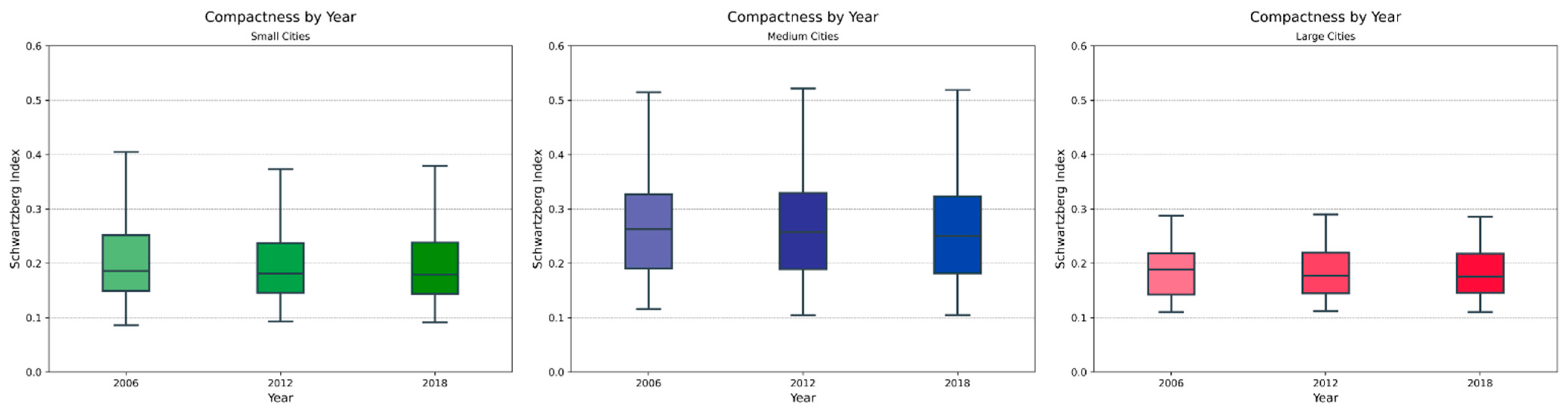
4.1.1. Compactness Index
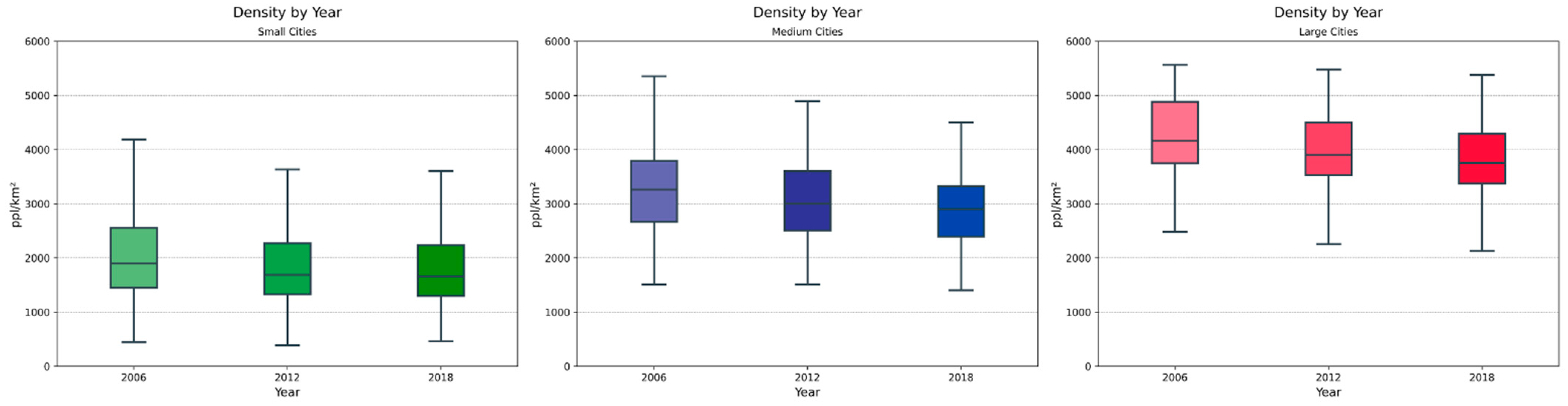
4.1.2. Urban Population Density
4.2. Correlation Analysis
4.2.1. Correlation between the Shrinkage/Growth Score and Compactness Index
4.2.2. Correlation between the Shrinkage/Growth Score and Urban Population Density
5. Findings and Discussion
- Addressing H1. There is a statistically significant correlation between compactness and shrinkage of medium-sized Polish cities.
- Addressing H2. There is a statistically significant correlation between urban population density and shrinkage of medium-sized Polish cities.
- Addressing H3. The trend persists within the analysed timeframe.
5.1. Urban Shape Compactness and Urban Shrinkage
5.2. Urban Population Density and Urban Shrinkage
5.3. Changes in Time
5.4. Planning Implications
5.5. Research Limitations
5.6. Implications for Further Research
6. Conclusions
Supplementary Materials
Author Contributions
Funding
Institutional Review Board Statement
Informed Consent Statement
Data Availability Statement
Conflicts of Interest
Appendix A
Appendix A.1. Shrinking Score

| Parameter Id | Description |
|---|---|
| P1 | Total population of municipality |
| P2 | Inward and outward migration |
| P3 | Population in working age |
| P4 | Employed persons in municipality |
| P5 | Registered unemployed persons |
| P6 | Municipality’s own revenue |
| Unit Id | Teryt Id | Name | Level | Kind | Year | Population |
|---|---|---|---|---|---|---|
| 011212161011 | 1261011 | Kraków | 6 | 1 | 2006 | 756,267 |
| 011212161011 | 1261011 | Kraków | 6 | 1 | 2007 | 756,583 |
| 011212161011 | 1261011 | Kraków | 6 | 1 | 2008 | 754,624 |
| 011212161011 | 1261011 | Kraków | 6 | 1 | 2009 | 755,000 |
| 011212161011 | 1261011 | Kraków | 6 | 1 | 2010 | 757,740 |
| 011212161011 | 1261011 | Kraków | 6 | 1 | 2011 | 759,137 |
| 011212161011 | 1261011 | Kraków | 6 | 1 | 2012 | 758,334 |
| 011212161011 | 1261011 | Kraków | 6 | 1 | 2013 | 758,992 |
| 011212161011 | 1261011 | Kraków | 6 | 1 | 2014 | 761,873 |
| 011212161011 | 1261011 | Kraków | 6 | 1 | 2015 | 761,069 |
| 011212161011 | 1261011 | Kraków | 6 | 1 | 2016 | 765,320 |
| 011212161011 | 1261011 | Kraków | 6 | 1 | 2017 | 767,348 |
| 011212161011 | 1261011 | Kraków | 6 | 1 | 2018 | 771,069 |
| 011212161011 | 1261011 | Kraków | 6 | 1 | 2019 | 779,115 |
| 011212161011 | 1261011 | Kraków | 6 | 1 | 2020 | 779,966 |
| 011212161011 | 1261011 | Kraków | 6 | 1 | 2021 | 782,137 |
| Teryt Id | Year | Population | Difference | Rate | Mean | Score |
|---|---|---|---|---|---|---|
| 1261011 | 2006 | 756,267 | −362 | −0.000480 | −0.000440 | 2 |
| 1261011 | 2007 | 756,583 | 316 | 0.000418 | −0.000250 | 2 |
| 1261011 | 2008 | 754,624 | −1959 | −0.002590 | −0.000810 | 2 |
| 1261011 | 2009 | 755,000 | 376 | 0.000498 | −0.000640 | 2 |
| 1261011 | 2010 | 757,740 | 2740 | 0.003629 | 0.000293 | 3 |
| 1261011 | 2011 | 759,137 | 1397 | 0.001844 | 0.000758 | 3 |
| 1261011 | 2012 | 758,334 | −803 | −0.001060 | 0.000462 | 3 |
| 1261011 | 2013 | 758,992 | 658 | 0.000868 | 0.001155 | 3 |
| 1261011 | 2014 | 761,873 | 2881 | 0.003796 | 0.001814 | 3 |
| 1261011 | 2015 | 761,069 | −804 | −0.001060 | 0.000877 | 3 |
| 1261011 | 2016 | 765,320 | 4251 | 0.005586 | 0.001624 | 3 |
| 1261011 | 2017 | 767,348 | 2028 | 0.002650 | 0.002366 | 3 |
| 1261011 | 2018 | 771,069 | 3721 | 0.004849 | 0.003162 | 3 |
| 1261011 | 2019 | 779,115 | 8046 | 0.010435 | 0.004486 | 4 |
| 1261011 | 2020 | 779,966 | 851 | 0.001092 | 0.004917 | 4 |
| 1261011 | 2021 | 782,137 | 2171 | 0.002783 | 0.004357 | 4 |
| Teryt Id | Start | End | P1 | P2 | P3 | P4 | P5 | P6 | Total | Type |
|---|---|---|---|---|---|---|---|---|---|---|
| 1261011 | 2006 | 2011 | 3 | 3 | 0 | 2 | 2 | 2 | 12 | C |
| 1261011 | 2007 | 2012 | 3 | 3 | 0 | 2 | 0 | 2 | 10 | D |
| 1261011 | 2008 | 2013 | 3 | 3 | 0 | 2 | 0 | 2 | 10 | D |
| 1261011 | 2009 | 2014 | 3 | 3 | 0 | 2 | 0 | 2 | 10 | D |
| 1261011 | 2010 | 2015 | 3 | 3 | 0 | 2 | 0 | 2 | 10 | D |
| 1261011 | 2011 | 2016 | 3 | 3 | 1 | 3 | 0 | 2 | 12 | C |
| 1261011 | 2012 | 2017 | 3 | 4 | 1 | 3 | 1 | 2 | 14 | B |
| 1261011 | 2013 | 2018 | 3 | 4 | 1 | 3 | 1 | 2 | 14 | B |
| 1261011 | 2014 | 2019 | 4 | 4 | 2 | 3 | 2 | 2 | 17 | B |
| 1261011 | 2015 | 2020 | 4 | 4 | 3 | 3 | 1 | 2 | 17 | B |
| 1261011 | 2016 | 2021 | 4 | 4 | 3 | 3 | 0 | 2 | 16 | B |
Appendix A.2. Spatial Indexes
| Teryt Id | Year | District | |
|---|---|---|---|
| Area (km²) | Perimeter (km) | ||
| 1261011 | 2006 | 151,538,463 | 361,537 |
| 1261011 | 2012 | 167,952,975 | 317,358 |
| 1261011 | 2018 | 169,016,958 | 317,574 |
| Teryt Id | Year | Ci (Schwartzberg) |
|---|---|---|
| 1261011 | 2006 | 0.120702 |
| 1261011 | 2012 | 0.144760 |
| 1261011 | 2018 | 0.145119 |
| Teryt Id | Start | End | Population | CLC Year | District Area (km²) | Density (people/km²) |
|---|---|---|---|---|---|---|
| 1261011 | 2003 | 2008 | 757,685 | 2006 | 151,538,462 | 4999.95 |
| 1261011 | 2004 | 2009 | 757,430 | 2006 | 151,538,462 | 4998.26 |
| 1261011 | 2005 | 2010 | 756,629 | 2006 | 151,538,462 | 4992.98 |
| 1261011 | 2006 | 2011 | 756,267 | 2006 | 151,538,462 | 4990.59 |
| 1261011 | 2007 | 2012 | 756,583 | 2012 | 167,952,975 | 4504.73 |
| 1261011 | 2008 | 2013 | 754,624 | 2012 | 167,952,975 | 4493.06 |
| 1261011 | 2009 | 2014 | 755,000 | 2012 | 167,952,975 | 4495.30 |
| 1261011 | 2010 | 2015 | 757,740 | 2012 | 167,952,975 | 4511.62 |
| 1261011 | 2011 | 2016 | 759,137 | 2012 | 167,952,975 | 4519.93 |
| 1261011 | 2012 | 2017 | 758,334 | 2012 | 167,952,975 | 4515.15 |
| 1261011 | 2013 | 2018 | 758,992 | 2018 | 169,016,958 | 4490.62 |
| 1261011 | 2014 | 2019 | 761,873 | 2018 | 169,016,958.1 | 4507.672 |
| 1261011 | 2015 | 2020 | 761,069 | 2018 | 169,016,958.1 | 4502.915 |
| 1261011 | 2016 | 2021 | 765,320 | 2018 | 169,016,958.1 | 4528.066 |
Appendix A.3. Correlation Analysis
| Teryt Id | Name | Start | End | Score | Density (People/km²) | Ci (Schwartzberg) |
|---|---|---|---|---|---|---|
| 1261011 | Kraków | 2006 | 2011 | 12 | 4990.59 | 0.120702 |
| 1261011 | Kraków | 2011 | 2016 | 12 | 4519.93 | 0.144760 |
| 1261011 | Kraków | 2016 | 2021 | 16 | 4528.06 | 0.145119 |
References
- Haussermann, H.; Siebel, W. Die Schrumpfende Stadt und Die Stadtsoziologie; Springer: Berlin/Heidelberg, Germany, 1988; pp. 1–10. [Google Scholar]
- UN-HABITAT. Envisaging the Future of Cities. 2022. Available online: https://unhabitat.org/wcr/ (accessed on 20 March 2024).
- Pallagst, K.; Aber, J.; Audirac, I.; Cunningham-Sabot, E.; Fol, S.; Martinez-Fernandez, C.; Moraes, S.; Mulligan, H.; Vargas-Hernandez, J.; Wiechmann, T.; et al. The Future of Shrinking Cities: Problems, Patterns and Strategies of Urban Transformation in a Global Context; University of California: Berkeley, CA, USA, 2009. [Google Scholar]
- Wang, Y.; Liu, Y.; Zhou, G.; Ma, Z.; Sun, H.; Fu, H. Coordinated Relationship between Compactness and Land-Use Efficiency in Shrinking Cities: A Case Study of Northeast China. Land 2022, 11, 366. [Google Scholar] [CrossRef]
- Cunningham-Sabot, E.; Jaroszewska, E.; Fol, S.; Roth, H.; Stryjakiewicz, T.; Wiechmann, T. Processus de de’ croissance urbaine. In Villes et Régions Européennes en de’Croissance, Maintenir la Cohésion Territorial; Baron, M., Cunningham-Sabot, E., Grasland, C., Riviere, D., Van Hamme, G., Eds.; Editions Hermé: Barcelona, Spain, 2010. [Google Scholar]
- Martinez-Fernandez, M.C.; Wu, C.T. Shrinking cities in Australia. In Proceedings of the 3rd State of Australian Cities National Conference, Adelaide, Australia, 28–30 November 2007; pp. 28–30. [Google Scholar]
- Hollander, J.B. Polluted and Dangerous: America’s Worst Abandoned Properties and What Can Be Done about Them; University of Vermont Press: Burlington, ON, Canada, 2009. [Google Scholar]
- Koziol, M. Folgen des demographischen Wandels für die kommunale Infrastruktur, Deutsche Zeitschrift für Kommunalwissenschaften. Heft 2004, 43, 69–83. [Google Scholar]
- Pallagst, K.; Fleschurz, R.; Nothof, S.; Uemura, T. Shrinking cities: Implications for planning cultures? Artic. Urban Stud. 2021, 58, 164–181. [Google Scholar] [CrossRef]
- Reckien, D.; Martinez-Fernandez, C. Why do cities shrink? Eur. Plan. Stud. 2011, 19, 1375–1397. [Google Scholar] [CrossRef]
- Alves, D.; Barreira, A.P.; Guimarães, M.H.; Panagopoulos, T. Historical trajectories of currently shrinking Portuguese cities: A typology of urban shrinkage. Cities 2016, 52, 20–29. [Google Scholar] [CrossRef]
- Reis, J.P.; Silva, E.A.; Pinho, P. Spatial metrics to study urban patterns in growing and shrinking cities. Urban Geogr. 2016, 37, 246–271. [Google Scholar] [CrossRef]
- Rink, D.; Haase, A.; Bernt, M.; Großmann, K. Addressing Urban Shrinkage Across Europe—Challenges and Prospects, Shrink Smart. The Governance of Shrinkage within a European Context; Research Brief 1; Helmholtz Centre for Environmental Research: Leipzig, Germany, 2010; 25p. [Google Scholar]
- Haase, A.; Bontje, M.; Couch, C.; Marcinczak, S.; Rink, D.; Rumpel, P.; Wolff, M. Factors driving the regrowth of European cities and the role of local and contextual impacts: A contrasting analysis of regrowing and shrinking cities. Cities 2021, 108, 102–942. [Google Scholar] [CrossRef]
- Schwarz, N.; Haase, D.; Seppelt, R. Omnipresent Sprawl? A Review of Urban Simulation Models with Respect to Urban Shrinkage. Environ. Plan. B Plan. Des. 2010, 37, 265–283. [Google Scholar] [CrossRef]
- Stewart, J.Q. Suggested principles of “Social Physics”. Science 1947, 106, 179–180. [Google Scholar] [CrossRef]
- Schwartzberg, J.E. Reapportionment, Gerrymanders, and the Notion of Compactness. Minn. Law Rev. 1966, 50, 443–452. [Google Scholar]
- Batty, M.; Longley, P.A. Fractal-Based Description of Urban Form. Environ. Plan. B Plan. Des. 1987, 14, 123–134. [Google Scholar] [CrossRef]
- Kazimierczak, J.; Szafrańska, E. Demographic and morphological shrinkage of urban neighbourhoods in a post-socialist city: The case of Łódź, Poland. Geogr. Ann. Ser. B Hum. Geogr. 2019, 101, 138–163. [Google Scholar] [CrossRef]
- Turok, I.; Mykhnenko, V. East European Cities—Patterns of Growth and Decline, 1960–2005. Int. Plan. Stud. 2008, 13, 311–342. [Google Scholar]
- Großmann, K.; Bontje, M.; Haase, A.; Mykhnenko, V. Shrinking cities: Notes for the further research agenda. Cities 2013, 35, 221–225. [Google Scholar] [CrossRef]
- Liu, W.; Tong, Y.; Zhang, J.; Ma, Z.; Zhou, G.; Liu, Y. Hierarchical Correlates of the Shrinkage of Cities and Towns in Northeast China. Land 2022, 11, 2208. [Google Scholar] [CrossRef]
- Tan, Z.; Xiang, S.; Wang, J.; Chen, S. Identification and Measurement of Shrinking Cities Based on Integrated Time-Series Nighttime Light Data: An Example of the Yangtze River Economic Belt. Remote Sens. 2023, 15, 3797. [Google Scholar] [CrossRef]
- Yu, S.; Wang, R.; Zhang, X.; Miao, Y.; Wang, C. Spatiotemporal Evolution of Urban Shrinkage and Its Impact on Urban Resilience in Three Provinces of Northeast China. Land 2023, 12, 1412. [Google Scholar] [CrossRef]
- Siedentop, S.; Fina, S. Urban sprawl beyond growth: From a growth to a decline perspective on the cost of sprawl. In Proceedings of the 44th ISCOCARP Congress, Dalian, China, 19–23 September 2008. [Google Scholar]
- Schmidt, S.; Fina, S.; Siedentop, S. Post-socialist Sprawl: A Cross-Country Comparison. Eur. Plan. Stud. 2014, 23, 1357–1380. [Google Scholar] [CrossRef]
- Couch, C.; Karecha, J.; Nuissl, H.; Rink, D. Decline and sprawl: An evolving type of urban development—observed in Liverpool and Leipzig. Eur. Plan. Stud. 2005, 13, 117–136. [Google Scholar] [CrossRef]
- Schiller, P.; Kenworthy, J.R. An Introduction to Sustainable Transportation: Policy, Planning and Implementation, 2nd ed.; Earthscan: Oxford, UK, 2018. [Google Scholar] [CrossRef]
- Lityński, P. The Intensity of Urban Sprawl in Poland. ISPRS Int. J. Geo-Inf. 2021, 10, 95. [Google Scholar] [CrossRef]
- Couch, C.; Cocks, M.; Bernt, M.; Grossmann, K.; Haase, A.; Rink, D. Shrinking Cities in Europe. Town Ctry. Plan. 2012, 81, 264–270. [Google Scholar]
- Wolff, M.; Wiechmann, T. Uneven Urban Dynamics the Role of Urban Shrinkage and Regrowth in Europe; TU Dortmund University: Dortmund, Germany, 2018. [Google Scholar]
- Klaassen, L.H. Myśl I Praktyka Ekonomiczna A Przestrzeń; Wydawnictwo UŁ: Łódź, Poland, 1988. [Google Scholar]
- GUS. Polish Statistics. 2024. Available online: https://bdl.stat.gov.pl/bdl/start (accessed on 1 March 2023).
- GUS. Prognoza Ludności Rezydującej Dla Polski Na Lata 2023–2060; Departament Badań Demograficznych i Rynku Pracy GUS: Warszawa, Poland, 2023. Available online: https://stat.gov.pl/obszary-tematyczne/ludnosc/prognoza-ludnosci/prognoza-ludnosci-na-lata-2023-2060,11,1.html (accessed on 20 March 2024).
- Śleszyński, P. Wyznaczenie i typologia miast średnich tracących funkcje społeczno-gospodarcze. Przegląd Geogr. 2017, 89, 565–593. [Google Scholar] [CrossRef]
- Śleszyński, P. Aktualizacja Delimitacji Miast Średnich Tracących Funkcje Społeczno-Gospodarcze (Powiększających Dystans Rozwojowy); Instytut Geografii i Przestrzennego Zagospodarowania PAN: Warszawa, Poland, 2019. Available online: https://www.gov.pl/attachment/5c7a04a5-ab22-49e4--a6a1-e874ede01445 (accessed on 1 October 2023).
- Runge, A. Methodological problems associated with research on midsize towns in Poland. Prace Geogr. 2012, 129, 83–101. [Google Scholar] [CrossRef]
- Szymczyk, E.; Bukowski, M. Identification of shrinking cities in Poland using a multi-criterion indicator. Przegląd Geogr. 2023, 95, 447–473. [Google Scholar] [CrossRef]
- Milbert, A. Wachsen und Schrumpfen von Städten und Gemeinden 2013 bis 2018 im bundesweiten Vergleich; BBSR: Bonn, Germany, 2020; Available online: https://www.bbsr.bund.de/BBSR/DE/startseite/topmeldungen/downloads/wachsen-schrumpfen-hintergrund.pdf?__blob=publicationFile&v=2 (accessed on 10 July 2023).
- Tsai, Y.H. Quantifying urban form: Compactness versus ‘sprawl’. Urban Stud. 2005, 42, 141–161. [Google Scholar] [CrossRef]
- Squires, G.D. (Ed.) Urban Sprawl: Causes, Consequences, and Policy Responses; The Urban Institute Press: Washington, DC, USA, 2002. [Google Scholar]
- OECD. Compact City Policies A COMPARATIVE ASSESSMENT. 2012. Available online: https://www.oecd.org/greengrowth/compact-city-policies-9789264167865-en.htm (accessed on 20 March 2024).
- Dantzig, G.B.; Saaty, T.L. Compact City: A Plan for a Liveable Urban Environment; WH Freeman: New York, NY, USA, 1973. [Google Scholar]
- Ahlfeldt, G.; Pietrostefani, E. The Compact City in Empirical Research: A Quantitative Literature Review (SERC Discussion Paper). 2017. Available online: https://eprints.lse.ac.uk/83638/1/sercdp0215.pdf (accessed on 10 March 2024).
- Angel, S.; Arango Franco, S.; Liu, Y.; Blei, A. The shape compactness of urban footprints. Prog. Plan. 2020, 139, 100429. [Google Scholar] [CrossRef]
- Mouratidis, K. Compact city, urban sprawl, and subjective well-being. Cities 2019, 92, 261–272. [Google Scholar] [CrossRef]
- Guo, R.; Leng, H.; Yuan, Q.; Song, S. Impact of Urban Form on CO2 Emissions under Different Socioeconomic Factors: Evidence from 132 Small and Medium-Sized Cities in China. Land 2022, 11, 713. [Google Scholar] [CrossRef]
- He, Q.; Yan, M.; Zheng, L.; Wang, B.; Zhou, J. The Effect of Urban Form on Urban Shrinkage—A Study of 293 Chinese Cities Using Geodetector. Land 2023, 12, 799. [Google Scholar] [CrossRef]
- TERYT Database. Available online: https://eteryt.stat.gov.pl/eTeryt/rejestr_teryt/udostepnianie_danych/baza_teryt/uzytkownicy_indywidualni (accessed on 20 March 2024).
- Stryjakiewicz, T. Kurczenie się miast w europie środkowo-wschodniej. Rozw. Reg. I Polityka Reg. 2018, 24, 191–192. [Google Scholar]
- Cheshire, P. A new phase of urban development in Western Europe? The evidence for the 1980s. Urban Stud. 1995, 32, 1045–1063. [Google Scholar] [CrossRef]
- CIRES. Cities Regrowing Smaller. Fostering Knowledge on Regeneration Strategies in Shrinking Cities across Europe. 2022. Available online: http://cost-cires.eu/fileadmin/Conference/Presentations/02_Musterd.pdf (accessed on 1 January 2024).
- Jaroszewska, E. Urban Shrinkage and Regeneration of an Old Industrial City: The Case of Wałbrzych In Poland. Quaest. Geogr. 2019, 38, 75–90. [Google Scholar] [CrossRef]
- Sroka, B. Dychotomia Procesu Urbanizacji, Czyli Rozlewanie Miast Kurczących się w Kontekście Systemu Planowania Przestrzennego; Instytut Rozwoju Miast i Regionów: Kraków, Poland, 2021. [Google Scholar]
- Milbert, A. Wachsen oder schrumpfen? BBSR-Analysen KOMPAKT 2015, 12, 1–24. Available online: https://www.bbsr.bund.de/BBSR/DE/veroeffentlichungen/analysen-kompakt/2015/AK122015.html (accessed on 1 October 2023).
- CLC Database. Available online: https://land.copernicus.eu/en/products/corine-land-cover (accessed on 20 March 2023).
- European Environment Agency. Corine Land Cover Nomenclature Guidelines. 2019. Available online: https://land.copernicus.eu/content/corine-land-cover-nomenclature-guidelines/docs/pdf/CLC2018_Nomenclature_illustrated_guide_20190510.pdf (accessed on 23 July 2024).
- Cieślak, I.; Biłozor, A.; Szuniewicz, K. The Use of the CORINE Land Cover (CLC) Database for Analyzing Urban Sprawl. Remote Sens. 2020, 12, 282. [Google Scholar] [CrossRef]
- Śleszyński, P.; Gibas, P.; Sudra, P. The Problem of Mismatch between the CORINE Land Cover Data Classification and the Development of Settlement in Poland. Remote Sens. 2020, 12, 2253. [Google Scholar] [CrossRef]
- GUGiK Database. Available online: https://www.gov.pl/web/gugik (accessed on 20 March 2024).
- Mubareka, S.; Koomen, E.; Estreguil, C.; Lavalle, C. Development of a composite index of urban compactness for land use modelling applications. Landsc. Urban Plan. 2011, 103, 303–317. [Google Scholar] [CrossRef]
- Niemi, R.G.; Grofman, B.; Carlucci, C.; Hofeller, T. Measuring Compactness and the Role of a Compactness Standard in a Test for Partisan and Racial Gerrymandering. J. Politics 1990, 52, 1155–1181. [Google Scholar] [CrossRef]
- Altman, M. The Consistency and Effectiveness of Mandatory District Compactness Rules. Chapter 2 of Districting Principles and Democratic Representation. Ph.D. Thesis, California Institute of Technology, Pasadena, CA, USA, 1998. Available online: https://thesis.library.caltech.edu/1871/3/2chapter_2.pdf (accessed on 5 May 2024).
- Chambers, C.; Miller, A. A Measure of Bizarreness. Q. J. Political Sci. 2010, 5, 27–44. [Google Scholar] [CrossRef]
- Barnes, R.; Solomon, J. Gerrymandering and Compactness: Implementation Flexibility and Abuse. Political Anal. 2021, 29, 448–466. [Google Scholar] [CrossRef]
- Cohen, J.; Cohen, P.; West, S.G.; Aiken, L.S. Applied Multiple Regression/Correlation Analysis for the Behavioural Sciences, 3rd ed.; Routledge: London, UK, 2002. [Google Scholar]
- Onwuegbuzie, A.J.; Daniel, L.G. Uses and misuses of the correlation coefficient. Res. Sch. 2002, 9, 73–90. [Google Scholar]
- Dong, T.; Jiao, L.; Xu, G.; Yang, L.; Liu, J. Towards sustainability? Analyzing changing urban form patterns in the United States, Europe, and China. Sci. Total Environ. 2019, 671, 632–643. [Google Scholar] [CrossRef] [PubMed]
- EUROSTAT. Available online: https://ec.europa.eu/eurostat/statistics-explained/index.php?title=Living_conditions_in_Europe_-_housing (accessed on 20 March 2024).
- Xu, G.; Zhengzi, Z.; Limin, J.; Zhao, R. Compact Urban Form and Expansion Pattern Slow Down the Decline in Urban Densities: A Global Perspective. Land Use Policy 2020, 94, 104563. [Google Scholar] [CrossRef]
- Schwaab, J. Sprawl or compactness? How urban form influences urban surface temperatures in Europe. City Environ. Interact. 2022, 16, 100091. [Google Scholar] [CrossRef]
- Newman, P.; Kosonen, L.; Kenworthy, J. Theory of urban fabrics: Planning the walking, transit/public transport and automobile/motor car cities for reduced car dependency. Town Plan. Rev. 2016, 87, 429–458. [Google Scholar] [CrossRef]
- Newman, P.W.G.; Kenworthy, J.R. Sustainability and Cities: Overcoming Automobile Dependence; Island Press: Washington, DC, USA, 1999; p. 442. [Google Scholar]
- Newman, P.; Kenworthy, J. The End of Automobile Dependence: How Cities are Moving Away from Car-Based Planning; Island Press: Washington, DC, USA, 2015; p. 273. [Google Scholar]
- Hollander, J.; Johnson, M.; Drew, R.B.; Tu, J. Changing urban form in a shrinking city. Environ. Plan. B Urban Anal. City Sci. 2019, 46, 963–991. [Google Scholar] [CrossRef]


| Index | Characteristic | Summary |
|---|---|---|
| A | Economic density | Refers to the number of economic agents living or working within a spatial unit and is typically measured as population or employment density (Thomas and Cousins 1996; Churchman 1999; Burton 2002; Neuman 2005). |
| B | Morphological density | Refers to the density of the built environment and captures aspects of the compact city such as compact urban land cover, demarcated limits (demarcated urban/rural land borders), street connectivity, impervious surface coverage, and a high building footprint to parcel size ratio (OECD 2012; Wolsink 2016; Neuman 2005; Burton 2002; Churchman 1999). |
| C | Mixed land use | Captures the co-location of employment, residential, retail and leisure opportunities (Churchman 1999; Burton 2002; Neuman 2005), both horizontally across buildings and vertically within buildings Burton (2002). |
| CLC Code | Name | |
|---|---|---|
 | 111 | Continuous urban fabric |
 | 112 | Discontinuous urban fabric |
 | 121 | Industrial or commercial units |
 | 122 | Road and rail networks and associated land |
 | 123 | Port areas |
 | 124 | Airports |
 | 131 | Mineral-extraction sites |
 | 132 | Dump sites |
 | 133 | Construction sites |
 | 141 | Green urban areas |
 | 142 | Sport and leisure facilities |
| Code | Class Name |
|---|---|
| B | Housing |
| Ba | Industrial |
| Bi | Other built-up areas |
| Bp | Urbanised areas with no buildings |
| Bz | Recreation areas |
| K | Mining areas |
| dr | Transport areas—Roads |
| Tk | Transport areas—Rail |
| Ti | Transport areas—other |
| Top |
Areas designated for future infrastructure investments |
| Schwartzberg Compactness Index Outcomes Per Year | 2006 | 2012 | 2018 |
|---|---|---|---|
| Number of observations | 180 | 184 | 180 |
| Min | 0.1160 | 0.1047 | 0.1049 |
| Median | 0.2628 | 0.2577 | 0.2503 |
| Max | 0.5146 | 0.5221 | 0.5186 |
| Urban Population Density Outcomes Per Year | 2006 | 2012 | 2018 |
|---|---|---|---|
| Number of observations | 180 | 184 | 180 |
| Min (ppl/km²) | 1511 | 1512 | 1406 |
| Median (ppl/km²) | 3259 | 3000 | 2903 |
| Max (ppl/km²) | 5353 | 4893 | 4502 |
| Name of the City | Urban Population Density Based on the Authors’ Calculation for ‘Artificial Surfaces’ for CLC2012 (people/km²) | Urban Population Density Sourced from GUS BDL for 2013 (people/km²) |
|---|---|---|
| Wieliczka (6, 3) | 2134 | 3634 |
| Jasło (6, 1) | 2357 | 3568 |
| Bartoszyce (6, 1) | 3809 | 4295 |
| Śrem (6, 3) | 3156 | 2877 |
| Leszno (6, 1) | 3307 | 4164 |
| Wejherowo (6, 1) | 5735 | 5847 |
| Sopot (6, 1) | 5614 | 5582 |
| Trzebinia (6, 3) | 1617 | 2926 |
| Polkowice (6, 3) | 1513 | 1231 |
| Periods | |||
|---|---|---|---|
| 2006–2011 | 2011–2016 | 2016–2021 | |
| Number of observations | 180 | 184 | 180 |
| Correlation for “urban fabric” | 0.09 (p = 0.21) | −0.07 (p = 0.32) | −0.06 (p = 0.4) |
| Correlation for “artificial surfaces” | 0.05 (p = 0.44) | −0.08 (p = 0.235) | −0.08 (p = 0.252) |
| Periods | |||
|---|---|---|---|
| 2006–2011 | 2011–2016 | 2016–2021 | |
| Number of observations | 147 | 149 | 147 |
| Correlation for “urban fabric” | 0.34 (p = 0.00) | 0.23 (p = 0.00) | 0.22 (p = 0.005) |
| Correlation for “artificial surfaces” | 0.29 (p = 0.0002) | 0.19 (p = 0.014) | 0.18 (p = 0.024) |
| Periods | |||
|---|---|---|---|
| 2006 | 2012 | 2018 | |
| Number of observations | 33 | 35 | 33 |
| Correlation for “urban fabric” | 0.02 (p = 0.9) | −0.12 (p = 0.47) | 0.02 (p = 0.89) |
| Correlation for “artificial surfaces” | −0.017 (p = 0.923) | −0.074 (p = 0.67) | 0.064 (p = 0.72) |
| Periods | |||
|---|---|---|---|
| 2006–2011 | 2011–2016 | 2016–2021 | |
| Number of observations | 180 | 184 | 180 |
| Correlation for “urban fabric” | −0.29 (p = 0.000) | −0.27 (p = 0.000) | −0.20 (p = 0.005) |
| Correlation for “artificial surfaces” | −0.222 (p = 0.002) | −0.231 (p = 0.001) | −0.105 (p = 0.157) |
| Periods | |||
|---|---|---|---|
| 2006–2011 | 2011–2016 | 2016–2021 | |
| Number of observations | 147 | 149 | 147 |
| Correlation for “urban fabric” | −0.18 (p = 0.022) | −0.11 (p = 0.15) | −0.03 (p = 0.71) |
| Correlation for “artificial surfaces” | −0.081 (p = 0.32) | −0.016 (p = 0.83) | 0.12 (p = 0.14) |
| Periods | |||
|---|---|---|---|
| 2006–2011 | 2011–2016 | 2016–2021 | |
| Number of observations | 33 | 35 | 33 |
| Correlation for “urban fabric” | −0.24 (p = 0.16) | −0.26 (p = 0.11) | −0.18 (p = 0.31) |
| Correlation for “artificial surfaces” | −0.242 (p = 0.17) | −0.28 (p = 0.103) | −0.073 (p = 0.68) |
| Hypothesis | Selected Urban Areas (CLC Classes) | All Medium-Sized Municipalities (6, 1 and 6, 3) | Medium-Sized Urban Municipalities (6, 1) | Medium-Sized Urban-Rural Municipalities (6, 3) |
|---|---|---|---|---|
| H1: There is a statistically significant correlation between urban compactness and shrinkage. | “Urban fabric” | NO | YES | NO |
| “Artificial surfaces” | NO | YES | NO | |
| H2: There is a statistically significant correlation between urban population density and shrinkage. | “Urban fabric” | YES | Yes, for 2006–2011 | NO |
| “Artificial surfaces” | YES for 2006–2016 | NO | NO | |
| H3: The trend persists within the analysed timeframe. | “Urban fabric” | YES | YES (for compactness relationship only) | NO |
| “Artificial surfaces” | NO | YES (for compactness relationship only) | NO |
Disclaimer/Publisher’s Note: The statements, opinions and data contained in all publications are solely those of the individual author(s) and contributor(s) and not of MDPI and/or the editor(s). MDPI and/or the editor(s) disclaim responsibility for any injury to people or property resulting from any ideas, methods, instructions or products referred to in the content. |
© 2024 by the authors. Licensee MDPI, Basel, Switzerland. This article is an open access article distributed under the terms and conditions of the Creative Commons Attribution (CC BY) license (https://creativecommons.org/licenses/by/4.0/).
Share and Cite
Szymczyk, E.; Bukowski, M.; Kenworthy, J.R. Understanding the Relationship between Urban Form and Urban Shrinkage among Medium-Sized Cities in Poland and Its Implications for Sustainability. Sustainability 2024, 16, 7030. https://doi.org/10.3390/su16167030
Szymczyk E, Bukowski M, Kenworthy JR. Understanding the Relationship between Urban Form and Urban Shrinkage among Medium-Sized Cities in Poland and Its Implications for Sustainability. Sustainability. 2024; 16(16):7030. https://doi.org/10.3390/su16167030
Chicago/Turabian StyleSzymczyk, Ewa, Mateusz Bukowski, and Jeffrey Raymond Kenworthy. 2024. "Understanding the Relationship between Urban Form and Urban Shrinkage among Medium-Sized Cities in Poland and Its Implications for Sustainability" Sustainability 16, no. 16: 7030. https://doi.org/10.3390/su16167030
APA StyleSzymczyk, E., Bukowski, M., & Kenworthy, J. R. (2024). Understanding the Relationship between Urban Form and Urban Shrinkage among Medium-Sized Cities in Poland and Its Implications for Sustainability. Sustainability, 16(16), 7030. https://doi.org/10.3390/su16167030