Multi-Objective Optimization of Highway Work Zones Considering Safety, Mobility, and Project Cost

Abstract

The presence of highway work zones has a major effect on safety, mobility, and project expenses. The objective of this study is to develop a multi-objective optimization model to address these challenges by considering all three factors simultaneously. The model employs a Genetic Algorithm to identify the Pareto front and elucidate the trade-offs between safety, mobility, and cost. It evaluates various decision variables related to site geometry, work management, and temporary traffic control measures, exploring numerous potential combinations and offering decision-makers a comprehensive array of solutions. A case study demonstrates the model’s efficacy. Initially, approximately 829,440 feasible solutions were identified, which were effectively reduced to 263 by imposing additional constraints such as specific safety levels, maximum project costs, or traffic delay thresholds. The findings highlight significant cost variations: crash costs ranged from saving USD 973,473 to increasing costs by USD 1,328,322; mobility costs ranged from USD 184,491 to USD 3,854,212; and project costs ranged from USD 1,424,634 to USD 1,574,894. These variations underscore the substantial influence of crash costs and the benefits of location-based scheduling, which improves cost estimate reliability by capturing the effects of working hours and project duration. This research builds upon previous studies by incorporating three distinct objectives rather than focusing on a singular solution. By addressing safety, mobility, and project cost separately, the framework yields multiple solutions, each impacting the objectives differently. This multifaceted approach enhances its utility as a robust decision-making tool for stakeholders involved in highway work zone management and planning. This study concludes that multi-objective optimization is crucial for providing realistic and diverse solutions, ultimately improving decision-making processes in highway work zone operations.

1. Introduction

Highway work zones (HWZs) are essential for addressing two primary concerns: first, the imperative to address the aging infrastructure, as both safety and functionality degrade over time. Second, there is a need to accommodate the increased demand for travel by enhancing road capacity. However, while necessary, HWZs come with significant direct and indirect costs. Direct costs encompass substantial project expenses, which includes the use of temporary traffic control (TTC) and human control. Indirect costs manifest as time lost, which is a resource with economic value, as well as vehicle operation costs (VOCs) and emission expenses. Also, an increase in crash rates is noted as a characteristic of HWZs. These costs, both direct and indirect, can be categorized into three main areas: safety, mobility, and project costs.

In safety, numerous studies have explored the safety implications of HWZs for both motorists and highway workers. While many of these studies have indicated an increase in crash rates within HWZs [1,2,3], some have identified instances of lower crash rates at certain sites [4,5,6]. For instance, La Torre et al. [2] found that HWZs resulted in a 33% rise in expected fatal-and-injury crash frequency and a 66% increase in property-damage-only crash frequency. Conversely, Graham et al. [4] observed a decrease in crash rates during construction in 31% of the projects analyzed. A comprehensive review by Yang et al. [7] revealed that a majority of articles (18 out of 21) reported an increase in crash rates within work zones, and 14 out of 27 articles reported an increase in the severity. Regarding mobility and its externalities, about 10% of the congestion and 24% of the nonrecurring lost time are caused by HWZs on US highways [8]. These significant traffic disruptions lead to environmental, economic, and social impacts. Research by Huang et al. [9] demonstrated that HWZs substantially contribute to vehicle emissions and result in an approximate 3% increase in fuel consumption. Studies show that many crashes are caused by human errors [10,11,12]; this can be partially attributed to continual traffic congestion, which renders drivers frustrated, impatient, and angry. This frustration and impatience among drivers can lead to aggression towards road workers, as evidenced by findings from Debnath et al. [13] which documented incidents such as object throwing and threats against traffic controllers. Moreover, time spent in traffic carries economic value, and increased traffic delays represent a waste of economic resources. Lastly, in project cost, HWZs incur significant execution expenses, including material costs, equipment, labor wages, and site overheads. Additionally, there are costs associated with deploying TTC measures.

The literature on the quantification of HWZ costs commonly represents the impacts on safety, mobility, and project costs using six components: agency and TTC costs reflect work impacts; the monetary value of lost time, VOC, and emission costs capture mobility impacts; and crash costs address safety impacts. Shahin et al. [14] conducted a quantitative analysis of these six cost components, denominated in dollars. Additionally, they devised a HWZ optimization model aimed at minimizing the total cost, which is derived from the cumulative sum of these six cost elements. Expanding on this research, a multi-objective optimization model was devised, incorporating three objectives: project cost (encompassing agency and TTC costs), mobility cost (including lost time, VOC, and emission costs), and safety cost (comprising crash costs). This approach separates the six cost components into three distinct objectives, enhancing the efficiency in selecting the optimal HWZ solution (set of decision variables).

Several studies have constructed a multi-objective optimization model to assess the trade-offs among various objective functions related to HWZs. These functions encompassed one or more of the six cost components. In some studies, these objective functions were monetized, while in others, they were measured using different units. For instance, lost time was quantified as total vehicle hour delay in certain studies and monetized in others. Furthermore, in studies where project cost was among the objectives, some considered only agency costs, while others incorporated additional expenses such as lost time and crash costs. The objective functions and their respective measuring units across these studies are outlined in

Table 1. HWZ multi-objective optimization models.

Study	Objective Functions (Unit of Measure)
Fwa et al. [20]	Work production (day)
	Maintenance cost (USD)
	Pavement condition index (-)
Jiang and Adeli [15]	Combined cost of agency, lost time, and crash (USD)
	Lost time (vehicle–hour)
El-Rayes and Kandil [16]	Agency cost (USD)
	Project duration (day)
	Project quality (-)
Kandil et al. [21]	Agency cost (USD)
	Combined cost of lost time and crashes (USD)
Abdelmohsen and El-Rayes [22]	Combined cost of agency and TTC (USD)
	Lost time (vehicle–hour)
Abdelmohsen and El-Rayes [17]	Safety (%)
	Lost time (vehicle–hour)
Isikyildiz and Akcay [23]	Agency cost (USD)
	Project duration (day)
	Project quality (-)
Sindi and Agbelie [24]	Agency cost (USD)
	Service life (year)
Amândio et al. [25]	Agency cost (USD)

. For example, Jiang and Adeli [15] developed a model to optimize cost and lost time. Lost time was quantified as total vehicle hour delay and cost included agency, lost time, and crash costs. El-Rayes and Kandil [16] developed a model to optimize construction cost, duration, and quality. Quality was quantified based on many indicators like asphalt content, gradation, and surface smoothness, and cost included agency cost. Another example is Abdelmohsen and El-Rayes [17], who developed a model to optimize safety and lost time. Lost time was quantified as total vehicle hour delay and safety was quantified as total crash rate change by using the Highway Safety Manual’s [18] multiple crash modification factor (CMF) combining method, which multiplies all CMFs to find the total change in crash rate. Their optimized variables are the work zone layout parameters, including speed limits, construction start time, shoulder use, lateral clearance, workspace length, TTC method, and access and egress method. In addition to the studies presented in Table 1, Kang et al. [19] developed an online algorithm for variable-speed-limit control in HWZs, to maximize throughput that in turn minimizes crashes. The optimized variable is a set of variable-speed-limit controls. The results show that the model considerably increases throughput and decreases speed variance.

The present research expands upon Shahin et al.’s [14] earlier study by introducing a multi-objective optimization model that incorporates safety, mobility, and project cost as separate objectives, recognizing that a uniform solution may not be optimal for all HWZs. This approach yields multiple solutions that can impact objectives differently, enhancing its utility as a robust decision-making tool for HWZ management. Importantly, this study addresses a gap in the literature, as no prior research has integrated safety, mobility, and cost into a single HWZ multi-objective optimization model. Furthermore, apart from Shahin et al. [14], few studies have considered all six cost components, with many relying on simplified equations that result in significant discrepancies between calculated and actual costs, project durations, and optimal decision variables. For a detailed discussion, Shahin et al. [14] provide further insights into these issues.

The objective of this study is to develop a multi-objective optimization model for HWZs, specifically targeting safety, mobility, and project cost. Utilizing a Genetic Algorithm, it aims to identify optimal trade-offs among these objectives. Ultimately, the research aims to enhance decision-making tools for stakeholders involved in managing highway work zones.

2. Methods

This study aims to mitigate the negative effects that HWZs pose on the aforementioned 6 cost components. This objective was accomplished by devising a multi-objective optimization model for HWZ operations. The model utilizes a Genetic Algorithm process [26] to identify the Pareto front. The three objective functions are delineated in Equations (1)–(3), while optimization occurs within the constraints outlined in Equations (4)–(9). The objective function defines the cost components as the extra expenses resulting from the presence of HWZs compared to regular road operations. Consequently, some cost components may exhibit negative values. For instance, if optimal HWZ operation results in lower crash rates compared to normal operations, the crash cost would be negative, indicating savings in crash expenses attributable to the enhanced safety of the road section.

$$Work cost=AGC+TTCC$$

(1)

$$Mobility cost=LTS+VOC+EMC$$

(2)

$$Safety cost=CRC$$

(3)

s.t.

$$L{B}_i\le X_i\le U{B}_i i=1,2,\dots ,n$$

(4)

$$AGC+TCC\le B^{max}$$

(5)

$$D\le D^{max}$$

(6)

$$TCMF\le TCM{F}^{max}$$

(7)

$$LT\le L{T}^{max}$$

(8)

$$G\left(X\right)\le 0$$

(9)

where $AGC$ denotes the agency cost. $TTCC$ denotes the temporary traffic control cost.$\mathrm{LTC}$ denotes the lost time cost. $VOC$ denotes the vehicle operating cost.$EMC$ denotes the emission cost. $CRC$ denotes the crash cost. $X_i$ denotes the value of decision variable i. $L{B}_i$ and $U{B}_i$ denotes the lower and upper bounds of decision variable i. D denotes the project duration. $D^{max}$ and $B^{max}$ denote the maximum allowed project duration and available budget, respectively. TCMF denotes the total crash modification factor. $TCM{F}^{max}$ denotes the maximum acceptable value of this variable. LT denotes the lost time. $L{T}^{max}$ denotes the maximum acceptable value of this variable. X denotes the array of decision variables. $G\left(X\right)$ denotes the functions of the decision variables that define additional constraints, such as technical constraints or the geometric design of the HWZ.

The Pareto front comprises a set of solutions where none are superior to others in all three objectives simultaneously. This set of solutions significantly narrows down the pool of feasible options, offering decision-makers a manageable quantity of solutions to evaluate. For instance, the model might present a solution on the Pareto front with slightly lower project costs but significantly worse mobility and safety outcomes. In such cases, it may be preferable to accept slightly higher project costs to mitigate traffic delays and reduce crash risks. Furthermore, while transportation agencies aim to minimize their costs (agency and TTC), they must obtain approval for their HWZ operations from law enforcement and local authorities, whose objective is to minimize mobility and safety costs. Hence, the multi-objective optimization model facilitates the identification of a solution that minimizes all objectives simultaneously. This study extends the optimization model introduced by Shahin et al. [14] into a multi-objective framework. The six cost components (AGC, TTC, LTC, VOC, EMC, and CRC) and the decision variables are thoroughly quantified and detailed in that study. Here is a concise overview of the equations for the six cost components:

2.1. Agency Costs (AGCs)

The AGCs consist of material, equipment, wages, and site overheads (Equations (10)–(13)).

$$MC={{\displaystyle \sum }}_{j}M{Q}_j·MU{C}_j$$

(10)

$$EC={{\displaystyle \sum }}_d{{\displaystyle \sum }}_{j}EW{H}_{j,d}·EH{C}_j·\left(1+EN{F}_{j,d}·ENAC\right)$$

(11)

$$WC={{\displaystyle \sum }}_d{{\displaystyle \sum }}_{j}WW{H}_{j,d}·WH{C}_j·\left(1+WN{F}_{j,d}·WNAC\right)$$

(12)

$$AGC=MC+EC+WC+SC+IC·D$$

(13)

where $MC$, EC and $WC$ denote the material, equipment, and workers’ wage costs, respectively. $SC$ denotes the cost of preparing the shoulders as a travel lane. The index j signifies the working tasks within the project. $M{Q}_j$ and $MU{C}_j$ denote the material quantity used in the task and its unit cost, respectively. The index d signifies working days from the start of the work and for its entire duration. $EW{H}_{j,d}$ and $WW{H}_{j,d}$ denote the number of working hours for equipment and workers, respectively. $EH{C}_j$ and $WH{C}_j$ denote the corresponding hourly equipment costs and workers’ wages, respectively. $EN{F}_{j,d}$ and $WN{F}_{j,d}$ denote the fractions of nighttime hours for equipment and workers, respectively. ENAC and WNAC denote the corresponding additional costs of night work for equipment and workers, respectively. IC denotes the daily indirect cost. D denotes the project duration.

2.2. Temporary Traffic Control Cost (TTCC)

The TTC cost component extends the model presented in Abdelmohsen and El-Rayes [22]. It includes installing, removing, renting, buying, relocating, and maintaining TTC devices. It also includes wages for police and flaggers (Equations (14)–(16)). TTC costs include the cost of basic TTC that is required by law and the cost of optional TTC (that is not always required by law), such as Dynamic Speed Displays (DSDs), and photo enforcement. Previous studies emphasized the effects of TTC on safety and mobility [27,28]; thus, it highly affects all of the model’s three objectives.

$$ETCC=\left[INC+RENC+RELC+REMC+OTTC\right]·\left(1+N{F}_d·TENAC\right)$$

(14)

$$WTCC={{\displaystyle \sum }}_{d}W{H}_d\left[PHC+FHC\right]·\left(1+N{F}_d·TWNAC\right)$$

(15)

$$TTCC=ETCC+WTCC$$

(16)

where $ETCC$ and $WTCC$ are the TTC equipment costs and personnel wages, respectively. $RENC$ denotes the TTC daily rental cost. $RELC$ denotes the cost of relocating the TTC from one day to the next. $INSC$ and $REMC$ denote the installation and removal costs for a distance unit, respectively. OTTC denotes the cost of optional TTC. $W{H}_d$ denotes the number of working hours on day d. $PHC$ and $FHC$ are the police and flagger hourly wages, respectively.$N{F}_d$ denotes the fraction of nighttime work on day d. $TENAC$ and $TWNAC$ denote the corresponding night additional cost for TTC equipment and wages, respectively.

2.3. Lost Time Cost (LTC)

Extended travel durations through HWZs result from diminished travel speeds due to alterations in road layout and the congestion that arises from limited traffic capacity at HWZ bottlenecks. These traffic slowdowns may lead some of the flow to shift to alternative routes, thereby easing delays on the HWZ route but leading to longer travel times on the detour routes. (Equations (17) and (18)). A detailed description of LTC calculation is found in (14).

LT = QLT + RSLT

(17)

$$LTC=LT·{{\displaystyle \sum }}_y{F}_y·H{C}_y^{LT}$$

(18)

where QLT denotes the total queue lost time in the entire project. RSLT denotes the reduced travel speed lost time. The index y signifies the vehicle type (passenger cars, single-unit trucks, and combination trucks). $F_y$ denotes the fraction of the total traffic of vehicle type y. $H{C}_y^{LT}$ denotes the hourly cost rate of lost time of vehicle type y.

2.4. Vehicle Operation Cost (VOC)

VOC is associated with fuel and engine oil consumption, tire wear, repair and maintenance, and mileage-related depreciation. HWZs affect VOC through the changes in speeds and queue delays that they generate (Equations (19)–(22)). It is based on the NCHRP Report 133 method [29].

$$RVOC={{\displaystyle \sum }}_d{{\displaystyle \sum }}_t{{\displaystyle \sum }}_y{Q}_{t,d}·\left[\left(RU{C}_y\left(V_{t,d}^{norm}\right)-RU{C}_y\left(v_{t,d}\right)\right)·F_y\right]$$

(19)

$$SVOC={{\displaystyle \sum }}_d{{\displaystyle \sum }}_t{{\displaystyle \sum }}_y\left(Q_{t,d}^{up}\right)·SU{C}_y\left(V_{t,d}^{norm}\right)·F_y$$

(20)

$$IVOC={{\displaystyle \sum }}_d{{\displaystyle \sum }}_t{{\displaystyle \sum }}_{y}Q{D}_{t,d}·IU{C}_y·F_y$$

(21)

$$VOC=RVOC+SVOC+IVOC$$

(22)

where $RVOC$, $SVOC$ and $IVOC$ denote the VOCs of reduced speed, stopping, and idling time, respectively. $RU{C}_y$, $SU{C}_y$ and $IU{C}_y$ denote the vehicle unit VOC for reduced speeds, stopping, and idling time, respectively. The index t signifies a time interval. $Q_{t,d}$ denotes the demand traffic flow. $Q_{t,d}^{up}$ denotes the demand traffic flow in the upstream section approaching the bottleneck at the HWZ entrance point. $Q{D}_{t,d}$ denotes the queueing delay in interval t to all vehicles. $V_{t,d}$ denotes the travel speed. $V_{t,d}^{norm}$ denotes the normal travel speed in the section with no work.

2.5. Vehicle Emission Cost (EMC)

HWZs typically result in reduced vehicle speeds and increased traffic congestion, leading to fluctuations in pollution emission rates. These variations differ among vehicle types. Estimating these speed fluctuations and the number of vehicles affected by HWZs allows for estimating changes in pollutant emission rates caused by HWZs. Subsequently, these changes in pollutant emissions are evaluated in economic terms by considering the health risks associated with each pollutant. To assess the economic impact of HWZs on pollution, these changes in emission rates are monetized based on established metrics that quantify the health impacts of each pollutant (Equations (23)–(25)). This method ensures a comprehensive evaluation of the environmental and public health effects of HWZs. It is based on the Cal-B/C model [29].

$$REMC={{\displaystyle \sum }}_d{{\displaystyle \sum }}_t{Q}_{t,d}·\left(L_d^{wz}+L1\right)·{{\displaystyle \sum }}_y{{\displaystyle \sum }}_{k}P{C}_k\left[\left(E{R}_{y,k}\left(v_{t,d}\right)-E{R}_{y,k}\left(V_{t,d}^{norm}\right)\right)·F_y\right]$$

(23)

$$IEMC={{\displaystyle \sum }}_d{{\displaystyle \sum }}_t{Q}_{t,d}·\left({\displaystyle \frac{Q_{t,d}·VL}{2N}}\right)·{{\displaystyle \sum }}_y{{\displaystyle \sum }}_{k}P{C}_k\left[\left(E{R}_{y,k}\left(V_{t,d}^{ID}\right)-E{R}_{y,k}\left(V_{t,d}^{norm}\right)\right)·F_y\right]$$

(24)

$$EMC=REMC+IEMC$$

(25)

where $REMC$ and $IEMC$ are the emission cost of reduced speed and idling time, respectively. $L_d^{wz}$ denotes the workspace length on day d. $L1$ denotes the length from the start of the shoulder taper until the end of the downstream taper, excluding the workspace. $P{C}_k$ denotes the health damage cost of a unit of pollutant k. $E{R}_{y,k}$ denotes the emission rate per distance travel unit of pollutant k for vehicle type y. $VL$ denotes the average vehicle length. $V_{t,d}^{ID}$ denotes the travel speeds in the queue. N denotes the number of available lanes.

2.6. Crash Cost (CRC)

The calculation of crash costs associated with HWZ involves systematically assessing the impact on crash rates across various severity levels. Initially, the method estimates the differential in crash rates attributable to the HWZ presence. These estimates are then multiplied by corresponding crash costs, which vary depending on the severity of outcomes. Subsequently, the total cost is adjusted to reflect the number of affected vehicles influenced by the HWZ. This approach ensures a comprehensive evaluation of the economic implications arising from HWZ, incorporating both the change in crash frequency and severity-specific cost considerations. To estimate crash rates at the road segment preceding the HWZ, the Empirical Bayes approach is utilized. This method integrates historical accident records and the Safety Performance Functions (SPFs) suitable for the road section. Then, to account for the changes in crash rates due to HWZ presence (due to geometric changes, posted speed limit change, and different TTC usage) crash modification factors (CMFs) are implemented. Finally, these changes in crash rates are monetized based on the crash costs for different severity levels (Equations (26)–(28)). A detailed description of the CRC calculation is found in (14).

$$TCMF={{\displaystyle \prod }}_{m}CM{F}_{m,s}$$

(26)

$$K=\left({\displaystyle \frac{{{\displaystyle \sum }}_d{{\displaystyle \sum }}_t{Q}_{t,d}}{365·AADT}}\right)$$

(27)

$$CRC=K·TCMF·{{\displaystyle \sum }}_{s}EC{R}_s^{noWZ}·C{C}_s$$

(28)

where the index m signifies the countermeasure. The index s signifies the crash severity. $CM{F}_{m,s}$ denotes the crash modification factor. K denotes the exposed vehicles adjustment factor. AADT denotes the annual average daily traffic. $EC{R}_s^{noWZ}$ denotes the expected yearly number of crashes without HWZ implementation per kilometer. $C{C}_s$ are the crash costs.

2.7. Solution Assessment Procedure

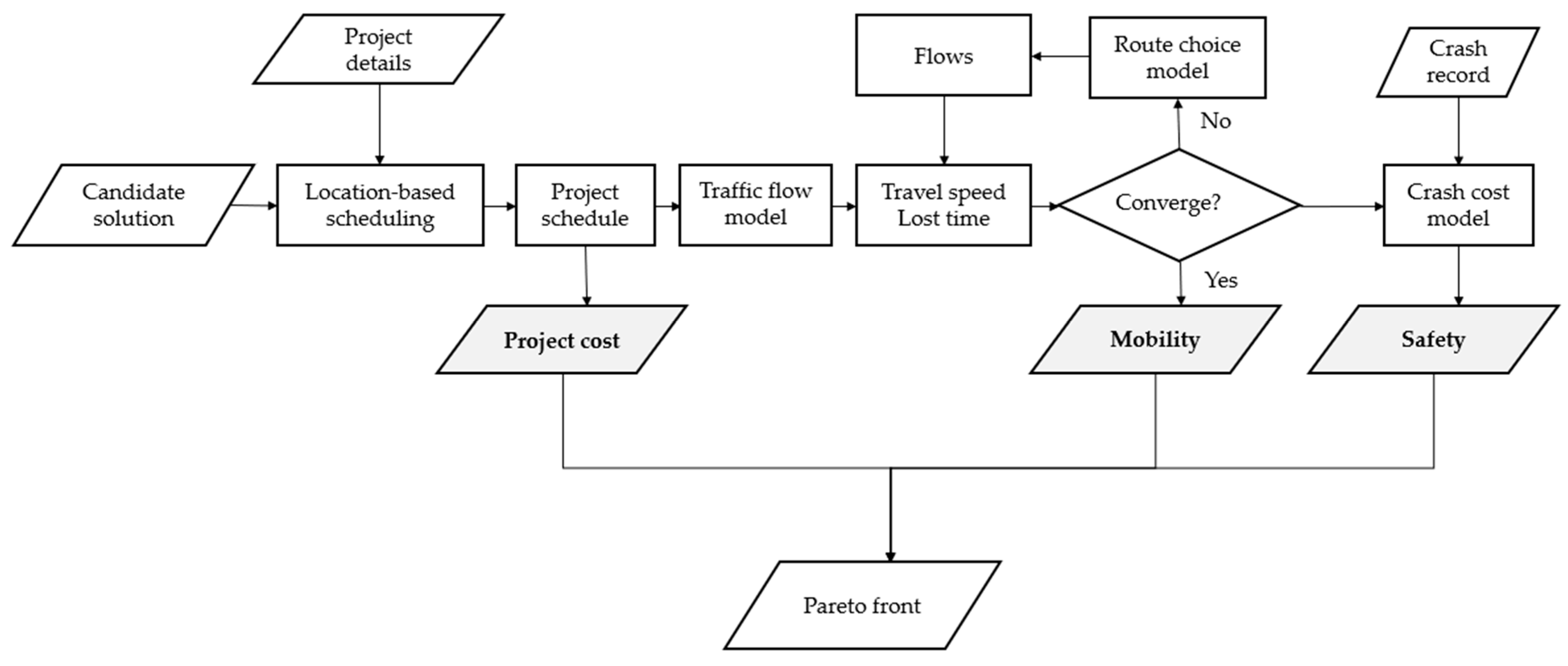
The method for assessing the objective function of a candidate solution (Figure 1) includes examining the site layout, work management strategies, and TTC decision variables, considering three distinct objectives: safety, mobility, and project cost. First, a project schedule is built based on the project’s characteristics, including the bill of quantities, tasks, time lags, crew formations, total length, and duration constraints, determining the project timeline, duration of tasks, length of work areas, hours allocated per task, and proportion of work conducted at night. Based on this, the agency and TTC costs are calculated (their sum is the project cost objective). The project timeline is integrated into the traffic flow model, which also includes traffic data for both the HWZ and alternative routes. Traffic delays at the HWZ may cause vehicles to divert to alternate routes, with these diversions assessed using a route choice model. The traffic flow model progressively adjusts its estimates for capacities, free-flow speeds, travel times, and queue delays on both HWZ and alternative routes until it achieves convergence. The final estimates of travel times and delays are then utilized to compute the costs associated with lost time, vehicle operations, and emissions (their sum is the mobility cost objective). Crash costs are calculated using these travel times and delays with the road crash record (safety objective). The process generates a Pareto front, representing trade-offs among safety, mobility, and project cost objectives, ensuring a balanced multi-objective evaluation for decision-makers. It also generates Pareto fronts between each two of the three objectives.

2.8. Case Study

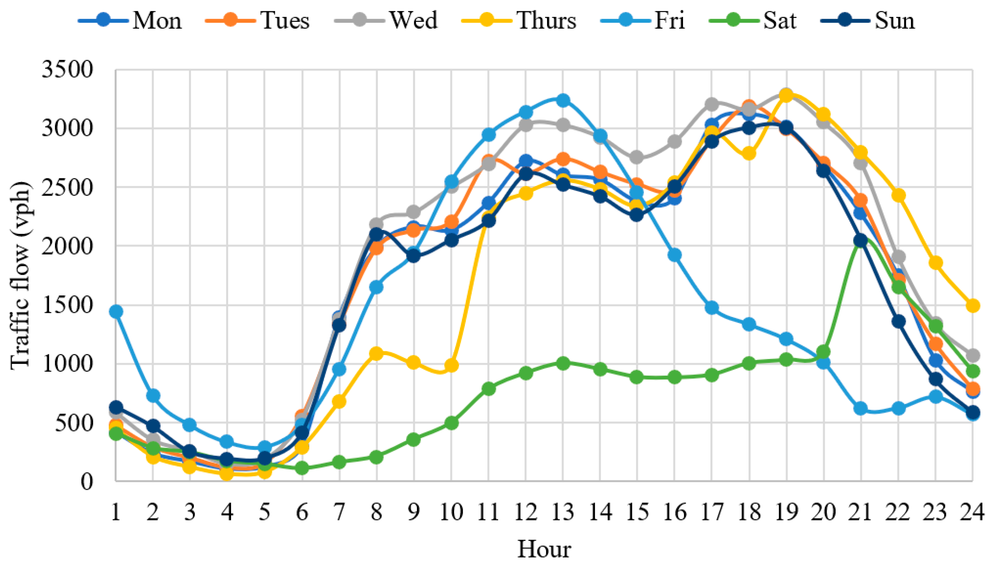
The case study entails a HWZ covering an 11.33 km road section in the rightmost lane of a single direction on a six-lane divided highway. The entirety of the road section will be closed for the duration of the project. Inputs and characteristics are summarized in

Table 2. Case study—input and characteristics.

Variable	Value	Source
Road geometry
Project total length	11.33 (km)
Original lanes width	3.6 (m)
Original shoulders width	1.8 (m)
Advanced warning area	750 (m)	[31]
Traffic modeling and economic impact of lost time
Rain	No	[32]
Base capacity and capacity adjustment factors		[32]
Base Free Flaw Speed and its adjustment factors		[29]
Heavy vehicle percentage	5%
AADT on one carriageway	50,000 (veh/day)
Daily and hourly traffic count		Road section in Israel
Passenger cars’s monetary value of travel time	21.89 (USD/veh–hr)	[29]
Heavy vehicles’s monetary value of travel time	23.06 (USD/veh–hr)
Alternative route additional travel time	No alternatives available
Crash data and costs
Fatal crash cost	9,100,000 (USD)	[33]
Injury crash cost	955,500 (USD)
Slight crash cost	27,300 (USD)
Fatal crash record for the entire section for the last 4 years	1 (crash/year)
Injury crash record for the entire section for the last 4 years	2 (crash/year)
Slight crash record for the entire section for the last 4 years	10 (crash/year)
TTC costs
VMS, DSD rental cost	700 (USD/month)
Photo enforcement	Initial cost: 50,000 Installation cost: 25,000 Monthly operating cost: 5000
Police wage	30 (USD/hour)	[34]
Flagger wage	12 (USD/hour)
VOC and emission costs
Vehicle unit VOC	NCHRP Report 133	[29]
Emission rates and health damage cost	Cal-B/C model

. Equation (29) [30] presents the SPF deemed appropriate for this project, with all CMFs sourced from [23]. A detailed breakdown of the traffic flow by day and hour is depicted in Figure 2. Project-specific data (

Table 3. Case study—Project tasks alternatives [31].

Task	Alternative for Task	Output (Unit/Day)	Material Cost (USD/Unit)	Labor Cost (USD/Day)	Equipment Cost (USD/Day)	Idle Time Cost (USD/Day)
Clear and grub (m2)	1	4000	0	900	1760	1300
Stripping topsoil (m3)	1	1220	0	490	806	600
	2	1400	0	550	950	720
	3	1560	0	670	1100	800
Earthmoving (m3)	1	1620	0	2300	4240	1800
	2	2140	0	2300	8360	2200
	3	2420	0	2300	9600	2600
Base (m2)	1	3760	8	2544	3470	1500
	2	3950	8	2740	3600	1700
	3	4100	8	2900	3850	1850
	4	4250	8	3150	4000	2000
Paving (m2)	1	4100	5	3320	1950	1200
	2	4250	5	3600	2200	1350

) has been sourced from [31], encompassing five consecutive tasks: clear and grub, stripping topsoil, earth moving, base construction, and paving. Each task can be carried out by several alternatives, each with its associated outputs, labor costs, equipment costs, and idle time costs. Idle time costs encapsulate expenses incurred when workers and equipment cease operations. An indirect cost of USD 3000 per day is assumed, inclusive of basic TTC expenses. El-Rayes [31] optimized the project cost using the A + B contracting method, wherein contractors are incentivized to minimize project duration by bidding on time, reflecting costs to the public such as travel congestion. In their study, they assumed a daily cost of USD 12,000. However, in the present case study, the A + B contracting method is not employed, and consequently, the “B” component will not factor into the optimization. Quantities pertinent to this case study are outlined in

Table 4. Case study—Work quantities.

Activity	Unit	Work Quantity
Clear and grub	m2	72,000
Stripping topsoil	m3	17,400
Earthmoving	m3	63,000
Base	m2	61,200
Paving	m2	61,200

, with a one-day time lag assumed between each consecutive task.

$$SP{F}_s=e^{10.4071}*AAD{T}^{-2.811}*e^{I_s}*AAD{T}^{0.1703*ln\left(AADT\right)}$$

(29)

where $I_s$ is the crash severity coefficient and is equal to −2.3926, −1.4845, and 0, assigned fatal, serious, and slight crashes, respectively. The uncertainty estimate for this SPF is 1.3984.

If idle time is not permitted, there are 72 potential crew formations for the project (derived from multiplying the number of alternatives for each task: 1 ∗ 3 ∗ 3 ∗ 4 ∗ 2 = 72, as shown in Table 3). However, the project allows for job breaks to expedite the project duration, albeit at the expense of increased agency costs. The only task in which a job break allows for a reduction in project duration (according to the basic principles of location-based scheduling) is the second task, stripping topsoil, since it comprises a fast task followed by a slow task. Consequently, for each of the 72 crew formations, a schedule is developed, allowing for a maximum job task break during stripping topsoil, resulting in a total of 144 potential crew formations.

Table 5. Decision variables lower and upper bounds and number of possible values.

	Lower Bound	Upper Bound	Number of Possible Values
Site layout geometry
Lane width (m)	2.7	3.3	3
Left shoulder width (m)	1.8	1.8	1
Lateral clearance (m)	0.3	0.9	Depends on lane width
TTC
Posted speed limit	50	90	5
VMS	0	1	2
Police patrol	0	1	2
Photo enforcement	0	1	2
Flagger presence	0	1	2
DSD	0	1	2
Access and egress	0	1	2
Work management
Work start day	Sunday	Friday	6
Tasks crew compositions	1	144	144

outlines the constraints on decision variables, defined by their lower and upper bounds, along with the number of potential values for each decision variable. Lane width and lateral clearance are adjusted in intervals of 0.3 m, while the posted speed limit is taken in 10 km/h intervals. No alterations to the left shoulder width were permitted (such as using it as a driving lane or increasing the lane width at its expense). Two access and egress methods are available, and no work is scheduled for Saturdays.

As previously stated, there were 144 possible crew formations considered. Notably, no constraints were imposed on the project budget, duration, total crash modification factor, or total lost time. While such restrictions would notably reduce the number of feasible solutions, they were intentionally omitted in this case study to comprehensively explore the impact of decision variables on each objective. Consequently, the study encompasses a total of 829,440 feasible solutions, obtained by multiplying the potential values of all decision variables. Despite the seemingly large number, this case study presents a relatively small number of feasible solutions.

3. Results and Discussion

The optimization process for the three-objective model identified 263 solutions, representing 0.03% of the total number of feasible solutions.

Table 6. Pareto front descriptive statistics.

	Crash Cost	Project Cost	Mobility Cost
Mean	(392,362)	1,498,411	1,400,834
Standard Error	27,777	2472	77,313
Median	(527,636)	1,500,144	957,232
Standard Deviation	450,468	40,083	1,253,802
Kurtosis	1.34	(1.13)	(0.78)
Skewness	1.32	(0.08)	0.84
Range	2,301,795	150,260	3,669,720
Minimum	(973,473)	1,424,634	184,491
Maximum	1,328,322	1,574,894	3,854,212

provides descriptive statistics for these solutions. The crash cost ranged from a saving of USD 973,473 to an increase in USD 1,328,322. Mobility cost varied between USD 184,491 and USD 3,854,212, while project cost ranged from USD 1,424,634 to USD 1,574,894. Engineers can reduce the number of potential solutions by applying thresholds to one or more of the three objectives. For instance, setting a mobility cost threshold of USD 200,000 reduces the pool of solutions to 23, offering a more manageable set of choices tailored to the project’s needs.

In terms of crash cost, the greatest savings were achieved using all optional TTC measures, as shown in Table 5. This solution required the maximum project duration of 51 days and a posted speed limit of 50 km/h, the lower bound. This solution also led to the highest mobility cost. Conversely, the highest crash cost solution involved no optional TTC measures and a project duration of 44 days, which also resulted in the lowest project cost.

For mobility cost, the lowest cost was attained by minimizing the project duration to 31 days, using no optional TTC measures, and setting the posted speed limit to 90 km/h, the upper bound. Regarding project cost, the highest cost scenario involved using all optional TTC measures, a project duration of 41 days, and a posted speed limit of 90 km/h. Although the difference between the maximum and minimum project costs is only about USD 50,000, this can be significant in projects with larger cost variations. The project duration differences are more pronounced, ranging from 31 to 51 days, which can substantially impact lost time, VOC, emissions, and crash cost components.

The TCMF measures the overall effect of chosen decision variables on the crash rate. However, crash cost is used to quantify the safety function rather than TCMF. This is because the lowest TCMF does not necessarily result in the fewest crashes, as project duration heavily influences this metric. For example, a HWZ layout with a TCMF of 1.2 may result in fewer crashes than a layout with a TCMF of 1.3 if the project duration is shorter.

To identify the trade-offs between each pair of the three objectives, the case study was solved for every two objectives while disregarding the third. For example, to find the trade-off between safety and mobility, the project cost was set to zero; therefore, it did not influence the optimization process. The findings are as follows:

3.1. Safety vs. Mobility

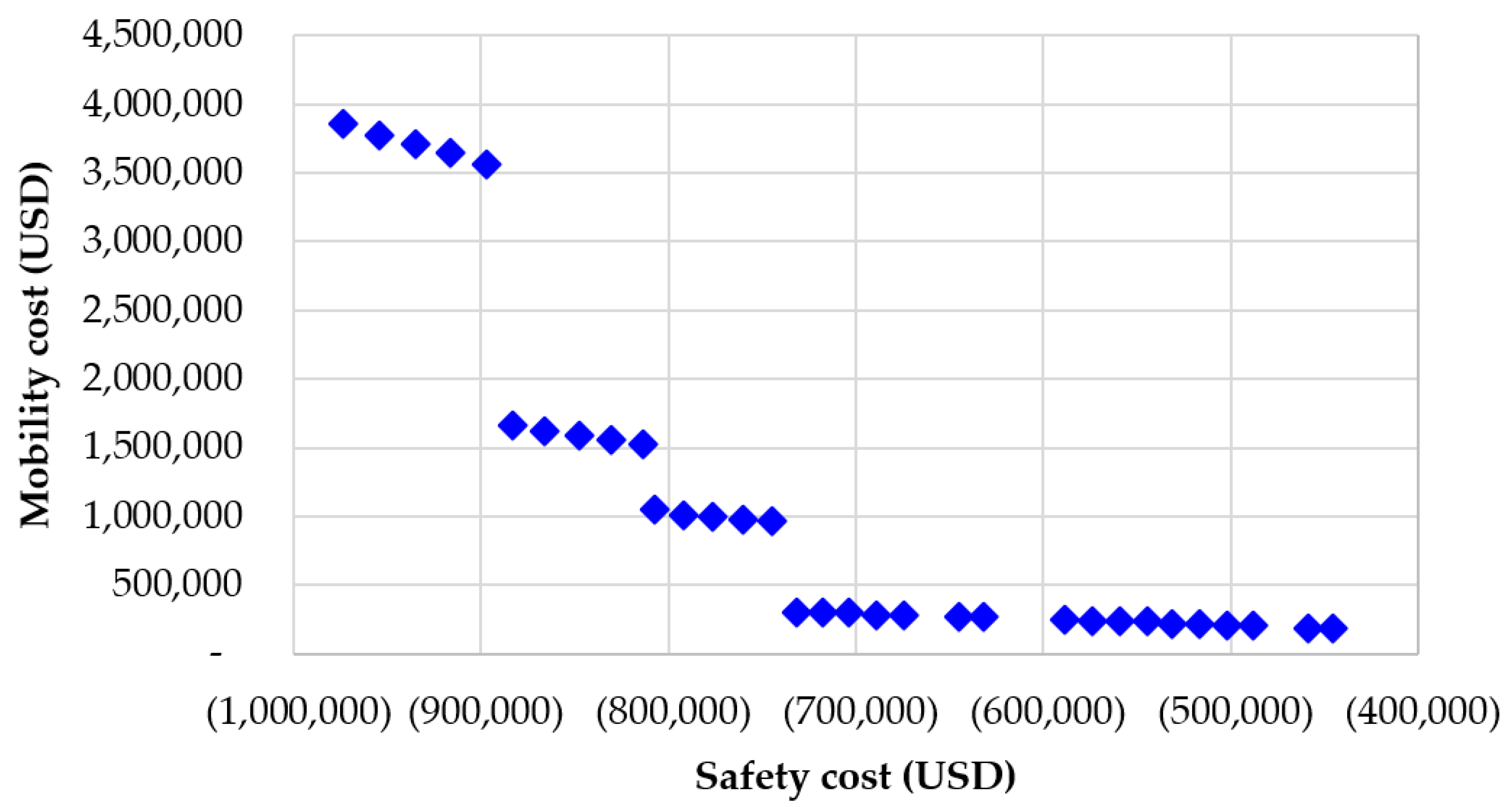
Figure 3 illustrates the Pareto front between crash cost and mobility cost, where the optimization process identified 32 solutions. In all these solutions, all optional TTC measures were employed, lane width was set at 3.3 m, lateral clearance at 0.3 m, and a flagger was used for access and egress. The variations among these solutions were in crew formation, posted speed limit, and the starting day of work. Different crew formations led to varying project durations, significantly affecting both crash and mobility costs. The starting days influenced the number of vehicles affected by the HWZ, impacting both mobility and safety. The posted speed limit accounted for the “steps” observed in Figure 3. The first five (leftmost) solutions had a posted speed limit of 50 km/h, resulting in the lowest crash risk but the highest mobility cost. The second group of five solutions had a posted speed limit of 70 km/h. The third group of five solutions had a posted speed limit of 80 km/h, and last 17 (rightmost) solutions had a posted speed limit of 90 km/h, resulting in the highest crash risk but the lowest mobility cost. The decrease in project duration within each group (e.g., from 51 to 47 days for the first group) led to descending trends in both crash cost savings and mobility costs. Longer project durations increased crash cost savings but also elevated mobility costs due to prolonged HWZ operations.

3.2. Work vs. Mobility

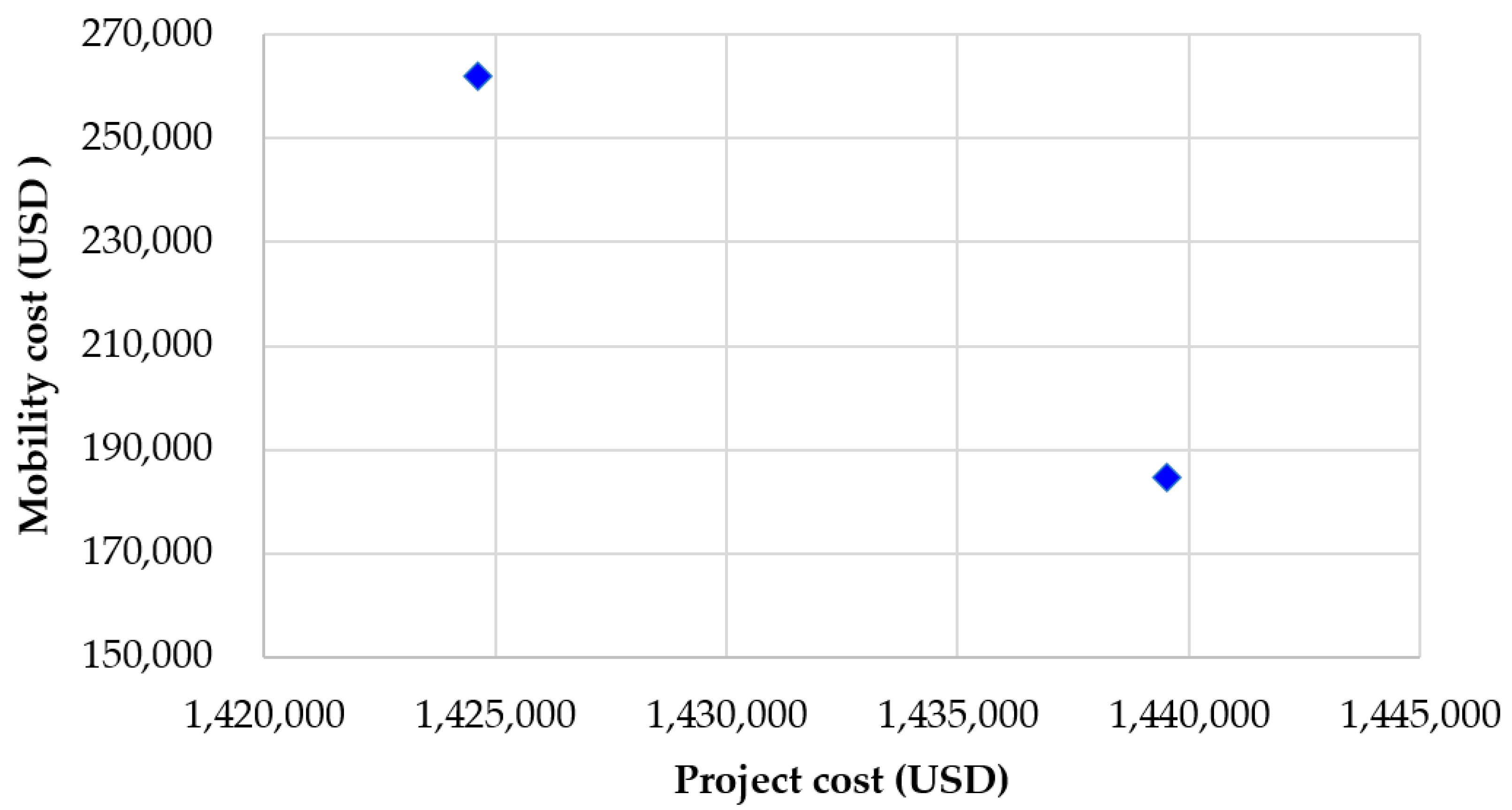
Figure 4 presents the Pareto front between project cost and mobility cost, revealing only two solutions. Both solutions involved no optional TTC measures, with lane width and lateral clearance set at 3.3 m and 0.3 m, respectively. Neither solution used a flagger for access and egress, and both maintained a speed limit of 90 km per hour to minimize mobility costs without impacting project costs. The main difference lies in crew formation and project duration: the left solution has a duration of 44 days, while the right solution has a duration of 31 days. The shorter project duration of 31 days results in lower mobility costs due to the reduced period of HWZ impact, but it incurs higher agency costs to achieve the shorter duration.

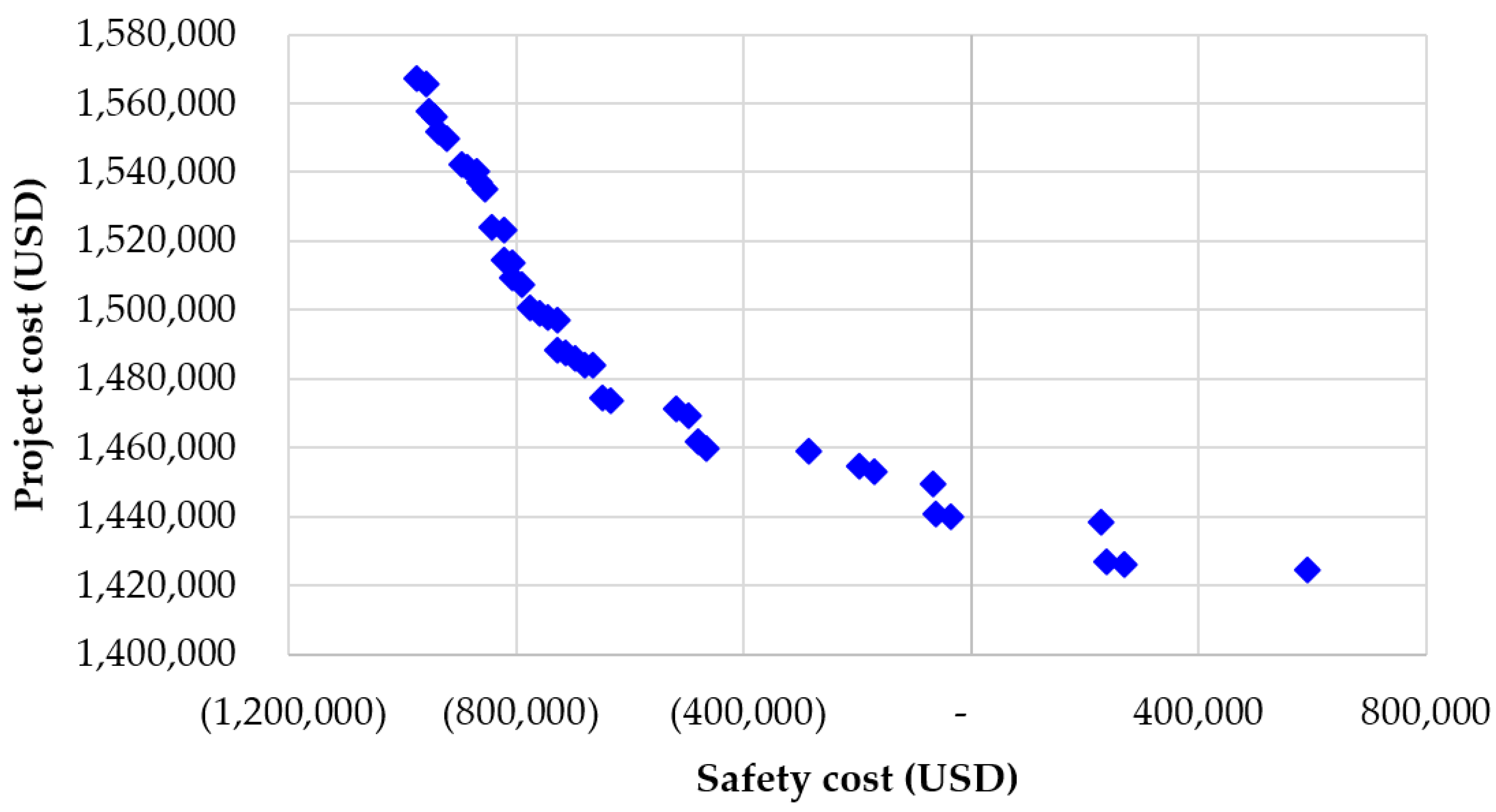
3.3. Safety vs. Work

Figure 5 depicts the Pareto front between safety cost and project cost. The optimization process identified 42 viable solutions, all maintaining lane widths of 3.3 m and lateral clearances of 0.3 m. A uniform posted speed limit of 50 km/h (the lower bound) was selected across all solutions to minimize speed-related risks, as speed limit variations do not impact project costs. Variations among the solutions arise from differences in optional TTC usage and crew formation, which affect project duration. The solution at the far left of the Pareto front has the lowest crash cost, achieved by using all optional TTC measures and having the longest project duration. Conversely, the solution at the far right has the highest crash cost due to the absence of optional TTC measures and the shortest project duration. Intermediate solutions utilize various combinations of optional TTC measures and project durations.

For example, using optional TTC measures such as VMS and DSD increases project costs but reduces safety costs by enhancing HWZ safety. Project duration significantly impacts project costs, with longer durations generally resulting in higher costs due to extended site overheads. Additionally, project duration affects the number of vehicles impacted by the HWZ. If the TTC measures provide safer conditions than those existing prior to the HWZ; a longer project duration can lead to substantial savings in crash costs.

The optimization results highlight the trade-offs between crash cost, mobility cost, and project cost in HWZ operations. By utilizing all optional TTC measures and varying crew formations, posted speed limits, and work starting days, the optimization process identified solutions that balance these three objectives. The Pareto front analyses (Figure 3, Figure 4 and Figure 5) demonstrate how different factors influence safety, mobility, and project costs.

• Safety vs. mobility: reducing posted speed limits minimizes crash risks but increases mobility costs, whereas higher speed limits have the opposite effect.
• Work vs. mobility: shorter project durations reduce mobility costs but increase project costs due to higher agency expenses.
• Safety vs. work: implementing comprehensive TTC measures and extending project duration reduces crash costs but increases project costs.

The novelty of this study is in developing a HWZ multi-objective optimization model that simultaneously considers safety, mobility, and cost. Previous studies have often relied on simplified equations for cost components, leading to significant deviations in actual total costs, project durations, and optimal sets of decision variables. Notably, crash cost has been often ignored or only included indirectly in previous works. However, our results underscore its critical importance, as it significantly impacts both HWZ costs and the selection of decision variables. Additionally, this study employs location-based scheduling, which improves the reliability of cost estimates by accounting for the effects of daily working hours and crew formation on work progress rates. This relationship is frequently overlooked in existing models, which typically assume a constant agency cost per unit of HWZ, disregarding the effects of crew formation and the number of working hours per day. By integrating these factors, the developed model provides a more accurate and realistic assessment of HWZ costs. However, the study had several imitations, such as the fact that the analysis assumes static traffic conditions and does not account for dynamic changes in traffic patterns over time. Also, the cost metrics used in this study may not fully capture the long-term economic impacts of HWZ operations. These limitations will be addressed in a future work to further refine the accuracy of the results.

4. Conclusions

A HWZ multi-objective optimization model considering safety, mobility, and project cost was developed. The model finds the Parto front for the three objectives, as well as the trade-offs between each two of the three objectives. To identify the optimal set of decision variables, a Genetic Algorithm was utilized that included site geometry, work management, and TTC. The present research builds upon an earlier study [14], extending its scope by incorporating three distinct objectives instead of one. Unlike the previous model, which offered a singular solution per project, this approach recognizes that a uniform solution may not be optimal for all HWZs. By addressing the diverse goals of safety, mobility, and project cost separately rather than as a singular entity, the framework yields multiple solutions, each potentially impacting the objectives differently. This multifaceted approach enhances its utility as a robust decision-making tool for stakeholders involved in HWZ management and planning. None of the previous studies developed a HWZ multi-objective optimization model that considered safety, mobility, and cost. Moreover, most studies made simplified equations of the cost components that led to significant deviations in the actual total cost, project duration, and optimal set of decision variables [14]. The model’s effectiveness is illustrated through a case study. The findings from the case study reveal the effectiveness of the multi-objective optimization model, providing decision-makers with a realistic quantity of solutions to examine based on the magnitude of each objective function and their perceived importance. Engineers can place thresholds on the three models’ objectives to whittle down the number of solutions to a manageable quantity. Crash costs significantly impact both project expenses and HWZ operations. Implementing location-based scheduling enhances the accuracy of cost estimates by directly accounting for the influence of working hours and project duration. Also, the effect of optional TTC on project cost and road safety was very apparent; it could lead to massive savings in crashes. The model contributes to sustainability by reducing environmental impact through decreased crash costs, enhancing economic efficiency with optimized project management, and improving social outcomes by increasing road safety and minimizing disruptions. This multifaceted approach supports the advancement of sustainable practices in highway work zone management. The limitations of the research include only considering one HWZ at a time, not considering all aspects of HWZ impacts, and using deterministic approaches to calculate traffic delays. A future work will consider the entire road network, estimating impacts like lost time and crashes, including diverted traffic. It will also include work quality, road service life, and preventative projects, and use microscopic models for better accuracy in estimating road capacity, traffic speed, and project lost time.