Article

Runoff Prediction of Tunxi Basin under Projected Climate Changes Based on Lumped Hydrological Models with Various Model Parameter Optimization Strategies

1
Hydrology and Water Resources Department, Nanjing Hydraulic Research Institute, Nanjing 210029, China
2
The National Key Laboratory of Water Disaster Prevention, Nanjing Hydraulic Research Institute, Nanjing 210029, China
*
Author to whom correspondence should be addressed.
Sustainability 2024, 16(16), 6897; https://doi.org/10.3390/su16166897
Submission received: 25 July 2024 / Revised: 7 August 2024 / Accepted: 9 August 2024 / Published: 11 August 2024
(This article belongs to the Section Sustainable Water Management)

Abstract

Runoff is greatly influenced by changes in climate conditions. Predicting runoff and analyzing its variations under future climates are crucial for ensuring water security, managing water resources effectively, and promoting sustainable development within the catchment area. As the key step in runoff modeling, the calibration of hydrological model parameters plays an important role in models’ performance. Identifying an efficient and reliable optimization algorithm and objective function continues to be a significant challenge in applying hydrological models. This study selected new algorithms, including the strategic random search (SRS) and sparrow search algorithm (SSA) used in hydrology, gold rush optimizer (GRO) and snow ablation optimizer (SAO) not used in hydrology, and classical algorithms, i.e., shuffling complex evolution (SCE-UA) and particle swarm optimization (PSO), to calibrate the two-parameter monthly water balance model (TWBM), abcd, and HYMOD model under the four objective functions of the Kling–Gupta efficiency (KGE) variant based on knowable moments (KMoments) and considering the high and low flows (HiLo) for monthly runoff simulation and future runoff prediction in Tunxi basin, China. Furthermore, the identified algorithm and objective function scenario with the best performance were applied for runoff prediction under climate change projections. The results show that the abcd model has the best performance, followed by the HYMOD and TWBM models, and the rank of model stability is abcd > TWBM > HYMOD with the change of algorithms, objective functions, and contributing calibration years in the history period. The KMoments based on KGE can play a positive role in the model calibration, while the effect of adding the HiLo is unstable. The SRS algorithm exhibits a faster, more stable, and more efficient search than the others in hydrological model calibration. The runoff obtained from the optimal model showed a decrease in the future monthly runoff compared to the reference period under all SSP scenarios. In addition, the distribution of monthly runoff changed, with the monthly maximum runoff changing from June to May. Decreases in the monthly simulated runoff mainly occurred from February to July (10.9–56.1%). These findings may be helpful for the determination of model parameter calibration strategies, thus improving the accuracy and efficiency of hydrological modeling for runoff prediction.

1. Introduction

According to the Sixth Assessment Report of the Intergovernmental Panel on Climate Change (IPCC) [1], the increase in global temperature is becoming more prominent, manifesting not only through significant increases in the intensity of extreme precipitation, but also in alterations to the hydrological cycle, particularly affecting runoff [2]. As a fundamental component of the hydrological cycle, studying runoff is a crucial step in scientifically understanding the hydrological cycle processes and comprehensively grasping the characteristics of water resources. Consequently, it is critical to estimate runoff changes under future climate scenarios.
To achieve this, ensuring an accurate simulation of catchment runoff is fundamental for effective water resource management [3,4]. As a vital tool for forecasting and managing water resources, process-based hydrological models such as the Hydrologiska Fyrans Vattenbalans modell (HBV) [5] and the Soil and Water Assessment Tool (SWAT) [6] have been used to simulate the elements of the hydrological cycle based on the understanding of the related causality of the water cycle [7]. Once the hydrological model and basin have been determined, the model’s performance is directly influenced by the rationality of the parameter calibration results [8,9]. The calibration of the hydrological model parameters can be regarded as an unconstrained optimization problem, while most of the model parameters are difficult to directly estimate because of the nonlinear structure of the models and the parameter uncertainty [10]. In addition, due to global warming and the change in hydrological factors such as precipitation and evapotranspiration, the runoff will increase the frequency and intensity of extreme events that cause the redistribution of water resources in time and space [11]. The latest climate change project, Coupled Model Inter-comparison Project Phase 6 (CMIP6), provides multiple datasets for the impacts of climate change on hydrological processes [12,13,14]. For example, Lei et al. [15] analyzed the hydrological changes using two lumped hydrological models under CMIP5 and CMIP6 climate model projections over 343 basins in China. Thus, it is essential to develop and select appropriate parameter calibration methods for researching future climate change and its impact on runoff at the watershed scale.
Over the past few decades, as computer technology has advanced rapidly, the optimization algorithms for automatically determining hydrological model parameters have replaced manual searches and have become the most common and effective technique [16,17,18,19]. In general, optimization algorithms can be classified into deterministic and stochastic algorithms according to the obtained solutions [20]. The deterministic algorithm follows rigorous mathematics programming to determine the optimal solution with the characteristic of the same input always corresponding to the same output. This algorithm is suitable for relatively simple problems with continuous space, but performs poorly for hydrological models due to its nonlinearity and non-differentiability. However, the stochastic algorithm can obtain different solutions in the process of searching during the same input. The heuristic algorithm is a primary stochastic algorithm that determines the optimal solution by mimicking the behavioral patterns of nature or living organisms. It has been widely used for parameter calibration in most basins worldwide. Moreover, the rapid development of computers has also directly contributed to optimization algorithms, with new or improved optimization methods appearing almost every year [21]. Advanced algorithms such as shuffling complex evolution (SCE-UA) [22], particle swarm optimization (PSO) [23], cuckoo search (CS) [24], and sparrow search algorithm (SSA) [25] have been proposed one by one with satisfactory convergence accuracy and speed, significantly improving the efficiency of the hydrological model parameter calibration. Recently, Wei et al. [26] proposed a new global optimizer for calibrating hydrological models, namely strategic random search (SRS), and demonstrated its robustness, wide applicability, and stability in hydrological model calibration. Moreover, some algorithms have been designed to solve problems in finance, economics, and engineering. For example, the gold rush optimizer (GRO) [27] and snow ablation optimizer (SAO) [28], derived from the process of gold-seekers prospecting for gold and the sublimation, melting, and evaporation behavior of snow, respectively, can yield better performance than classical algorithms for engineering problems.
Another crucial challenge for hydrological model parameter calibration is the selection of the objective functions [29,30]. Parameter calibration aims to estimate the optimal parameter value by comparing the model output and observations, so the selected objective function should be able to fully quantify simulation performance. Traditionally, statistical metrics such as the average root mean square error (RMSE) [31], Nash–Sutcliffe efficiency (NSE) [32], and Kling–Gupta efficiency (KGE) [33] are widely used as the objective functions for hydrological model parameter calibration, while they are sensitive to data distribution and extreme values. To address the above shortcomings, some methods or improvement indicators such as Box–Cox transformation [34], multi-objective calibration [35], and the sum of absolute errors (SAR) [36] have been applied in the model calibration. In addition, many researchers have tried to use hydrological characteristics to replace the above metrics for model parameter calibration and have found that they can improve the reliability of parameter estimation [37,38,39]. However, most hydrologists still tend to select traditional metrics as objective functions. It is worth noting that conventional objective functions have classical statistical moments in formulations, leading to the limitation of model calibration for non-normal distributions of data in hydrological modeling. A new method, namely, knowable moments (KMoments), combining the strengths of classical and L-moments, was proposed recently by Koutsoyiannis [40]. KMoments can obtain the reliable and effective estimation of high-order statistics in typical hydrologic samples. According to this, Pizarro et al. [41] introduced a new KGE variant relying on knowable moments (KMoments), and demonstrated that it can provide a more accurate simulation of hydrological processes.
Many researchers have noted the differences between new and classical stochastic optimization algorithms on hydrological model calibration [42,43,44]. However, most studies only focus on the hydrological models with a daily time step, and few studies on the applicability of the latest algorithms such as SRS and GRO for parameter calibration in monthly models, especially for future runoff prediction. However, the investigation of the KGE variant relying on knowable moments (KMoments) and considering high and low flows (HiLo) as the objective function in model parameter calibration is still rare, and the influence of different algorithms on its performance, especially the latest algorithms, e.g., SRS and GRO, remains to be explored. Thus, the new algorithms including SRS and SSA (used in hydrology), GRO and SAO (not used in hydrology), and classical algorithms, i.e., SCE-UA and PSO, are selected and applied in the TWBM, along with abcd and HYMOD model calibration (widely used for the simulation of monthly runoff in humid areas [45,46,47]) for monthly runoff simulation in Tunxi basin, China. Then, based on different objective functions, the effectiveness and stability of the above-mentioned algorithms for various models are evaluated to provide a reference for the selection of optimization algorithms for parameter calibration in hydrological models. Lastly, the future runoff of the Tunxi basin under projected climate changes is predicted via the hydrological model with the optimal parameter calibration scenario. This study can offer a reference for future water resource management in the Tunxi basin under climate change conditions.

2. Study Area and Data Sources
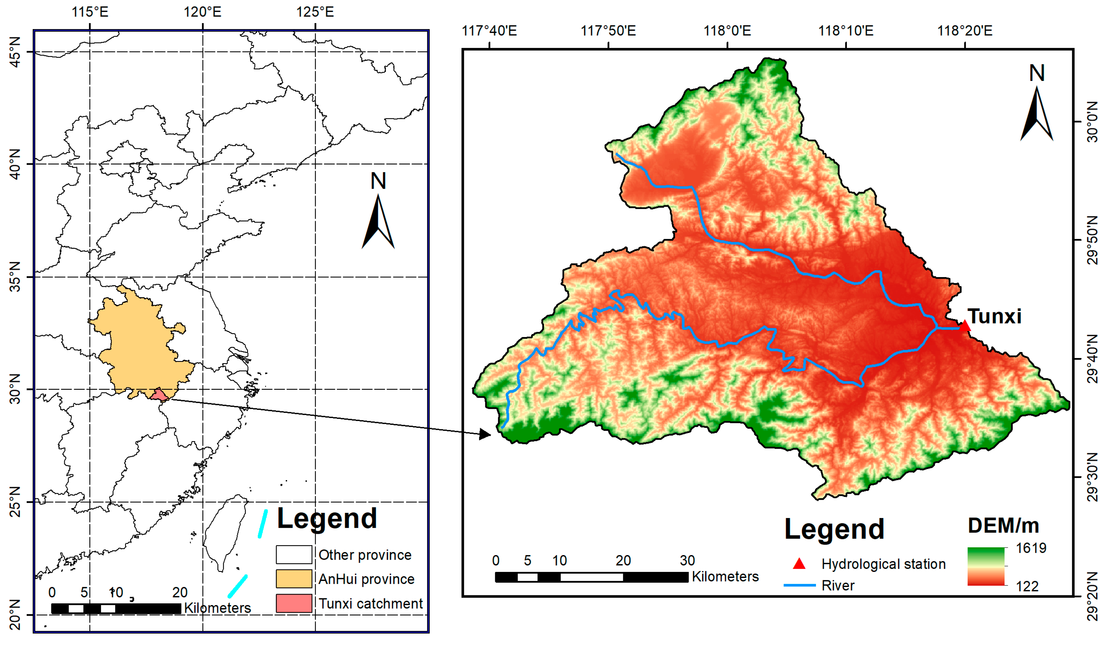
2.1. Study Area

The Tunxi (TX) catchment belongs to the Qiantang River system near the southeast of Anhui province, China. The TX catchment has a total drainage area of 2754 km2 and is located between the longitudes 117°36′ E–118°30′ E and latitudes 29°24′ N–118°06′ N. According to Figure 1, the basin’s terrain is high in the west and low in the east, with the lowest point being 122 m and the highest at 1619 m. It is located in a subtropical monsoon climate zone with a humid climate, and rainfall is mainly concentrated during the flood season from June to September. It is a typical small and medium basin in humid areas, China. Runoff varies with seasonal and inter-annual variability in the basin. The average annual rainfall and average annual temperature are about 1600 mm and 17 °C [48].

2.2. Hydrometeorological Data

The hydrometeorological data used in this study include monthly precipitation P, potential evapotranspiration PET, and runoff Q, which were obtained from the local Hydrological Bureau with time ranges from 1956 to 2000. Note that the first 70% of the above sequences were used for model calibration and the last 30% for model validation.

2.3. GCM Data

According to the applicability of CMIP6 data in China, six GCMs including CanESM5, FGOALS-g3, GFDL-ESM4, INM-CM5-0, IPSL-CM6A-LR, and MPI-ESM1-2-HR under two emission scenarios of SSP245 and SSP585 were applied for future runoff prediction in this study [49,50]. A brief description of the GCMs is listed in Table 1. The SSP245 scenario represents an intermediate level of greenhouse gas emissions, reflecting a moderate degree of social vulnerability and radiative forcing. In contrast, the SSP585 scenario depicts a high-forcing scenario, characterized by significant social vulnerability and high greenhouse gas emissions. It is the only pathway to reach a man-made radiative forcing level of 8.5 W/m2 by 2100.
To eliminate the systematic bias caused by coarse spatial resolution and the GCM model, the quantile mapping (QM) method was utilized to downscale the GCM output by applying a transfer function between the model outputs and observations, converting them from a coarse grid to a finer scale. The monthly precipitation and potential evapotranspiration were bias-corrected based on the corresponding observations for the period of 1980–2014, which were obtained from the National Tibetan Plateau/Third Pole Environment Data Center [51,52,53] (https://data.tpdc.ac.cn/). The spatial resolution of six GCM model products and historical observations were resampled to 0.25° × 0.25° using bilinear interpolation before bias correction. The details of the QM method can be found in [54]. The period of 2041–2070 bias-corrected monthly P and PET from the GCMs of the CMIP6 was used for future runoff prediction after the evaluation of model parameter calibration strategies.

3. Methodology

Three hydrological models were used for monthly runoff simulations under four objective function scenarios to evaluate the robustness of six optimization algorithms.

3.1. Hydrological Models

Three hydrological models, including the two-parameter monthly water balance model (TWBM), abcd model, and HYMOD model, were used to simulate the monthly runoff. Descriptions of these models are presented as follows.
(a) TWBM model: The model (see Figure 2a) generalizes the relationship between each hydrological process or variable into an empirical function or expression to simulate the catchment hydrological process based on the principle of water balance [45]. Due to its simple structure and good performance, it has been widely used in monthly runoff simulation, especially in humid regions. The input of the model is monthly P and PET, and the output is monthly actual evaporation AET and runoff Q. The AET is calculated using the following formula:
A E T t = C × P E T t × tanh ( P t / P E T t )
where t is the time step, and C is the model parameter, which comprehensively reflects the variation of precipitation and evapotranspiration (see Table 2). Then, the monthly runoff can be calculated as follows:
Q t = S t 1 + P t A E T t × tanh [ ( S t 1 + P t A E T t ) / S C ]
where S is the soil water content, and SC is the model parameter, which represents the water storage capacity of the catchment (see Table 2). Finally, the soil water content is updated by using the following formula:
S t = S t 1 + P t A E T t Q t
(b) abcd model: Similarly, based on the principle of water balance, the model simulates the regional hydrological cycle with potential evapotranspiration and precipitation as driving factors to obtain hydrological elements such as runoff, AET, and soil water content. The key assumption of the model is that the evapotranspiration opportunity is nonlinearly related to the available water such that the evapotranspiration opportunity increases quickly with available water for water-limited conditions, but asymptotically approaches a maximum constant value for energy-limited conditions [55]. The nonlinear relationship can be described as:
Y i = W i + b 2 a W i + b 2 a 2 W i b a
where Y is the evapotranspiration opportunity; W is the water availability; and a and b are the model parameters, which represent the probability of runoff formation before soil saturation and the water storage capacity of the upper soil zone, respectively. The model includes the soil moisture and groundwater storage layers, as shown in Figure 2b, and only four parameters, a, b, c, and d (see Table 2). The details of the model can be found in the literature [46].
(c) HYMOD model: The model (see Figure 2c) uses an excess rainfall model for runoff production via the principle similar to the Probability Distributed Model (PDM), as described by Moore [56]. The core of runoff production is the water storage capacity curve of the catchment, which can be defined as:
F C = 1 1 C C m a x B e x p , C 0 ,   C m a x
where Cmax is the maximum catchment storage capacity, and Bexp is the degree of variability of water storage capacity. This structure is coupled with a Nash cascade featuring three quick-flow tanks and one slow-flow tank designed to allocate water. The input data necessary to carry out simulations are P and PET and its output is the runoff. The model consists of five parameters; a brief description and prior referenced ranges are shown in Table 2. Detailed model process descriptions can be found in the literature [57].

3.2. Model Parameter Calibration Scenarios

To evaluate the impact of parameter calibration strategies on runoff simulations, three monthly hydrological models are applied to the study area under scenarios combined with six optimization algorithms and four objective functions.

3.2.1. Optimization Algorithms

The six optimization algorithms, i.e., SRS, SSA, GRO, SAO, SCE-UA, and PSO, were used in this study. Brief descriptions of the algorithms are presented as follows.
(a) SRS algorithm: The SRS is a heuristic algorithm for solving unconstrained single-objective optimization problems. The global optimum of the objective function can be found by the contraction, translation, and appropriate expansion of the feasible region based on the algorithm. It consists of three parts: pre-exploration preparation, refined search for optimized solutions, and jumping out of local optimum. The algorithm has two core parameters: p (determining the number of search particles) and δ (determining the rate of the search area shrinks). The details can be found in the literature [26].
(b) SSA algorithm: The SSA is inspired by the foraging and anti-predatory behaviors of sparrows. It includes population initialization, seeker position, entrant position, and alert position update, and stops when reaching the maximum number of iterations or the preset target value. Due to its high optimality-seeking ability and fast convergence speed, it has been used to calibrate hydrological model parameters in recent years [58,59].
(c) GRO algorithm: The GRO, derived from the process of gold-seekers prospecting for gold, can obtain the optimal solution by modeling how gold miners search for gold in a riverbed [27]. It is mainly based on the five states of a gold prospector’s movement: exploration, core formation, main core, dispersion, and final decision stage. As the latest global optimization algorithm, it has a high convergence speed, search efficiency, and strong robustness, and can be applied to various optimization problems.
(d) SAO algorithm: The SAO is inspired by the sublimation, melting, and evaporation behavior of snow [28]. By emulating the natural movement of snow, it can efficiently search for optimal solutions with simplicity, high efficiency, and strong robustness. It consists of three stages, i.e., initialization, exploration, and exploitation, and has a dual-population mechanism, which is designed to realize the trade-off between exploiting and exploring the solution space without premature convergence.
(e) Classical algorithms: As the most commonly used algorithms in hydrological model parameter calibration, the SCE-UA and PSO algorithms can efficiently search in the global scope and obtain the optimized parameters [60,61,62]. Details can be found in the literature [22,23]. The core parameter settings of all algorithms are presented in Table 3, and other parameter values are by default.

3.2.2. Objective Functions

Four KGE-based objective functions [41], i.e., KGE, KGE high and low flows (KGE_HiLo), KGE knowable moments (KGE_KMoments), and KGE KMoments high and low flows (KGE_KMoments_HiLo), were used to evaluate their impacts on model calibration, especially for the combination of KMoments in objective functions. The KGE can be calculated as follows:
K G E = 1 ( r 1 ) 2 + ( a 1 ) 2 + ( β 1 ) 2
where r is the Pearson correlation coefficient; a is the ratio of standard deviations of simulated and observed streamflow; and β is the ratio of mean values of simulated and observed streamflow.
The KGE_HiLo computed in this study, as presented in Equation (7), is a combination of KGE and inverse KGE with a focus on the high and low flows:
K G E _ H i L o = K G E ( Q ) + K G E ( 1 / Q )
where Q represents the streamflow time series, while 1/Q represents the inverse streamflow time series.
According to the method of unbiased estimators of noncentral KMoments [41], the KGE_KMoments can be expressed as:
K G E _ K M o m e n t s = 1 ( K ^ 1 s K ^ 1 o 1 ) 2 + ( 2 K ^ 2 s / K ^ 1 s 2 K ^ 2 o / K ^ 1 o 1 ) 2 + ( ρ 1 ) 2
where K ^ 1 s and K ^ 1 o , respectively, represent the first KMoment of simulated and observed streamflow time series; and K ^ 2 s and K ^ 2 o , respectively, represent the second KMoment of simulated and observed streamflow time series. Therefore, KGE_KMoments_HiLo can be calculated similarly to Equation (7):
K G E _ K M o m e n t s _ H i L o = K G E _ K M o m e n t s ( Q ) + K G E _ K M o m e n t s ( 1 / Q )

3.3. Evaluation Metrics

The Nash–Sutcliffe Efficiency (NSE) and Root Mean Squared Error (RMSE) were used to evaluate the goodness of the runoff simulations after model calibration.
N S E = 1 t = 1 n Q s i m , t Q o b s , t 2 t = 1 n Q o b s , t Q ¯ o b s 2
R M S E = t = 1 n Q s i m , t Q o b s , t 2 n
where Q s i m , t and Q o b s , t are the simulated and observed monthly streamflow for the tth month, respectively; Q ¯ o b s , t is the mean values of the streamflow observations; and n is the time series length.

4. Results and Discussion

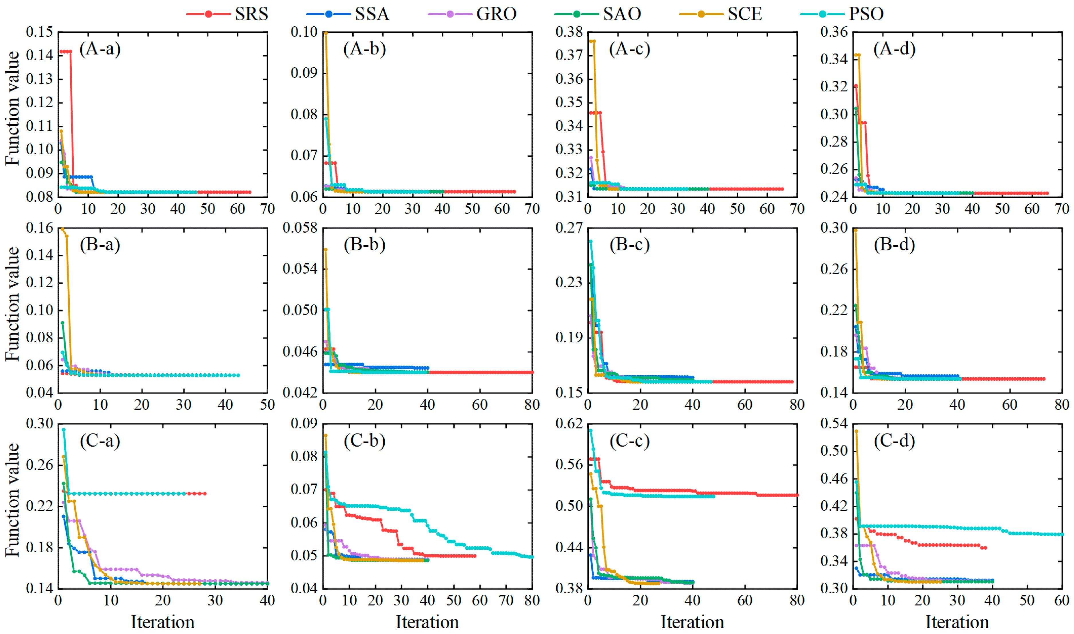
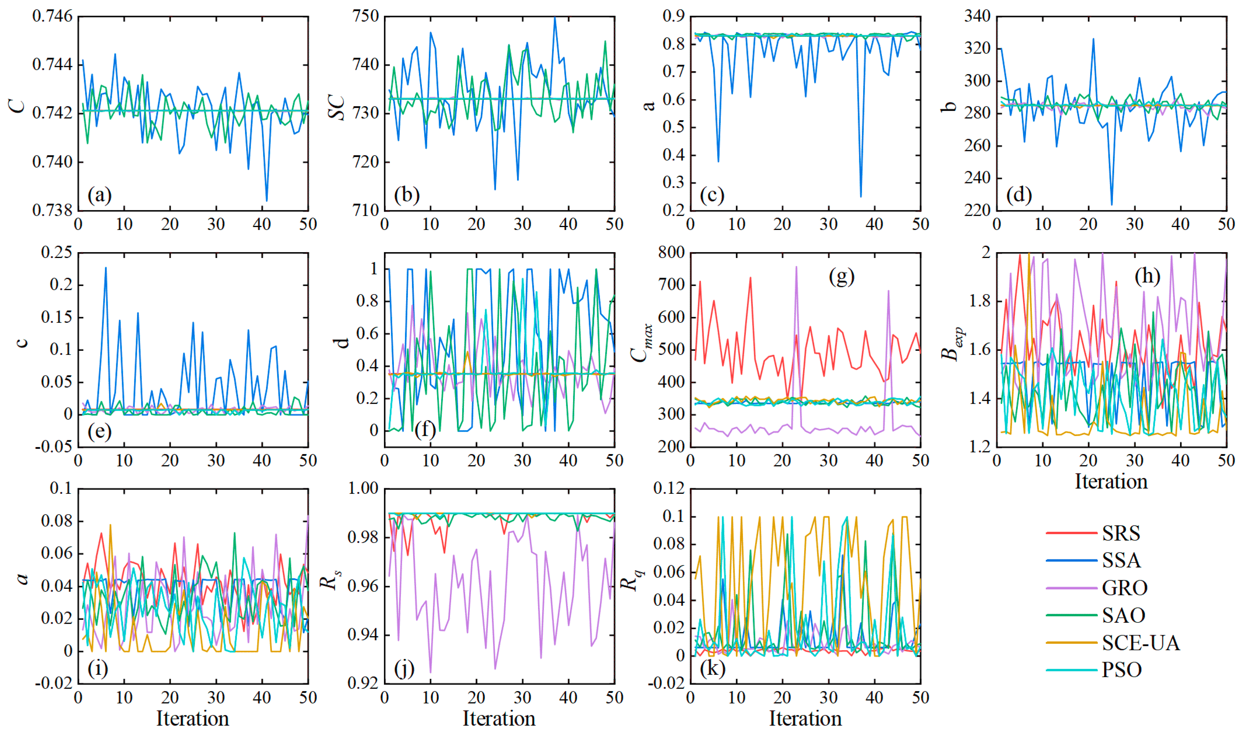
4.1. Efficiency Analysis under Parameter Calibration Scenarios

The plots in Figure 3 show the four objective function values for the TWBM, abcd, and HYMOD models using six optimization algorithms in the calibration period. For the TWBM and abcd models, all algorithms achieve almost the same convergence and become stable in about 10 iterations. However, the convergence and stability of the six algorithms are significantly different for the HYMOD model in that the convergence range of SRS and PSO algorithms is different from that of the others. It is worth noting that when KGE_KMoments is selected as the objective function, the SRS and PSO algorithms have a similar convergence with relatively low efficiency compared to the other algorithms. The results indicate that the efficiency of the HYMOD model calibration is closely related to the selection of objective function. Moreover, comparing the values of the four objective functions, KGE_KMoments has the smallest value, followed by KGE, KGE_KMoments_HiLo, and KGE_HiLo, which means that selecting KGE_KMoments as the objective function will most likely obtain the optimal parameters of the model.
Figure 4 further shows the radar chart of the evaluation metrics (NSE and RMSE) for validation with the TWBM, abcd, and HYMOD models considering the four objective functions and six optimization algorithms. Overall, the abcd and HYMOD models perform better than the TWBM model. Except for the results of HYMOD model calibration using the SRS and PSO algorithms with KGE_HiLo as the objective function, the NSE obtained by the rest is larger than 0.8, which also proves that the above three hydrological models can simulate the monthly runoff in humid areas [63]. Although the performance of the HYMOD model with the KGE_HiLo objective function shows a relatively worse result than the rest of the objective function scenarios, the NSE and RMSE for all hydrological models generally exhibit no significant difference under the six algorithms for model calibration, which indicates that the above algorithms can achieve the model calibration well using the appropriate objective function. Meanwhile, the abcd and HYMOD model calibration results with different objective functions and algorithms are similar, except for KGE_HiLo as the objective function for the HYMOD model calibration. However, there is a noticeable improvement in the performance of the TWBM model, with the NSE improving by a maximum of 0.079 and the RMSE decreasing by a maximum of 22.1% when KGE_KMoments_HiLo, KGE_HiLo, KGE, and KGE_KMoments are used in turn as objective functions. This implies that the abcd model is less affected by objective functions and algorithms, while the TWBM model is sensitive to the selection of the objective function.
Moreover, to evaluate the model improvement in the monthly simulation using KMoments and HiLo as objective functions, the performance of the three models with the four different objective functions and six optimization algorithms were summarized, as shown in Figure 5. It can easily be seen that the points are coincident in Figure 5A,B. Therefore, the correlation coefficient (r) was used to further evaluate the performance of model runoff simulation. The mean r of the TWBM model with KGE, KGE_KMoments, KGE_HiLo, and KGE_KMoments_HiLo as objective functions are 0.923, 0.938, 0.915, and 0.91, respectively. The mean r of the abcd model with KGE, KGE_KMoments, KGE_HiLo and KGE_KMoments_HiLo as objective functions are 0.955, 0.963, 0.957, and 0.957, respectively. For the HYMOD model (see Figure 5C), using KMoments as the objective function based on KGE_HiLo can effectively improve the model’s underestimation of runoff with an r from 0.923 to 0.969. These results suggest that considering KMoments based on KGE can play a positive role in the model calibration, while the effect of adding the high and low flows (HiLo) is unstable. A similar finding was also reported for the daily runoff simulation conducted by Pizarro et al. [41].

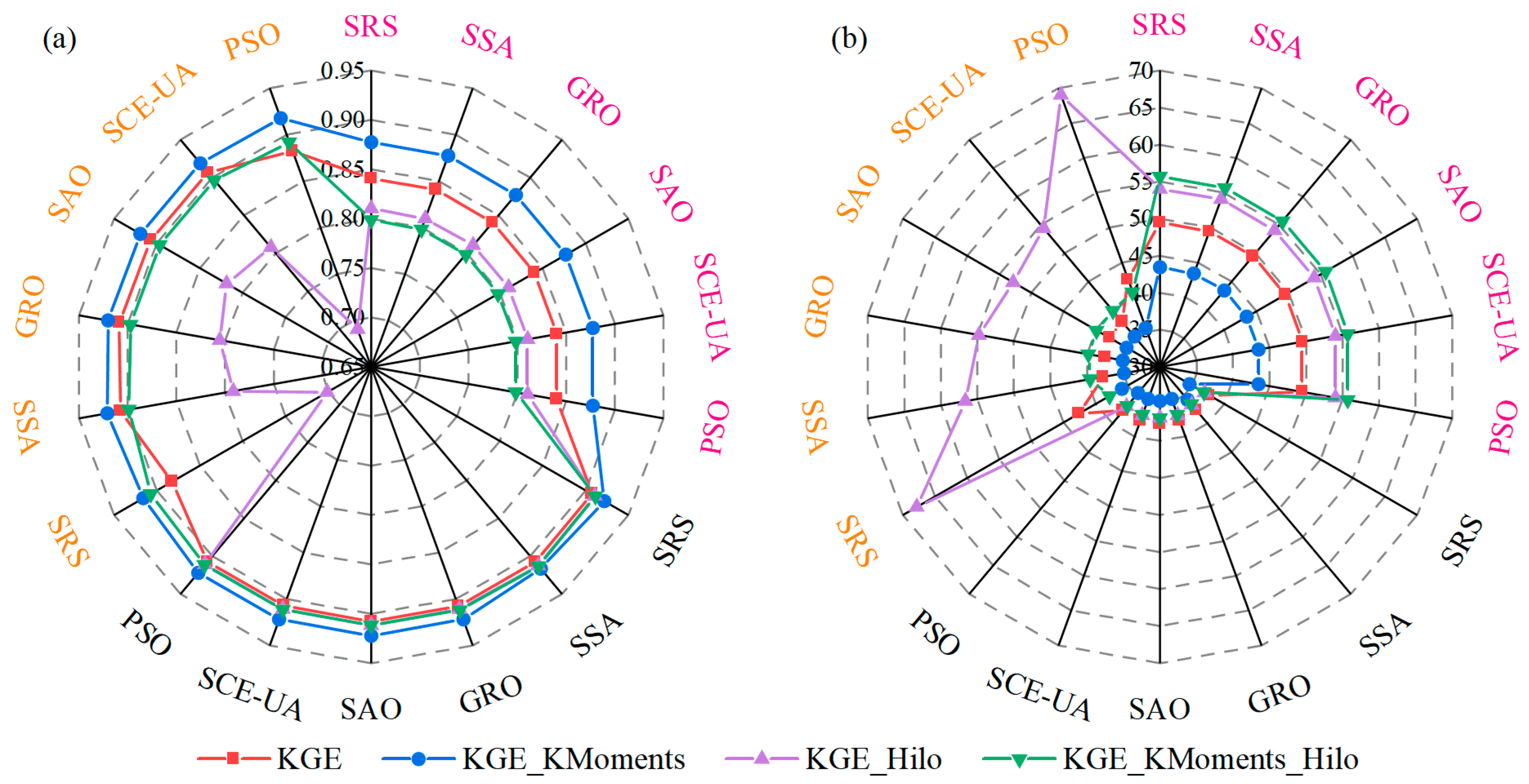
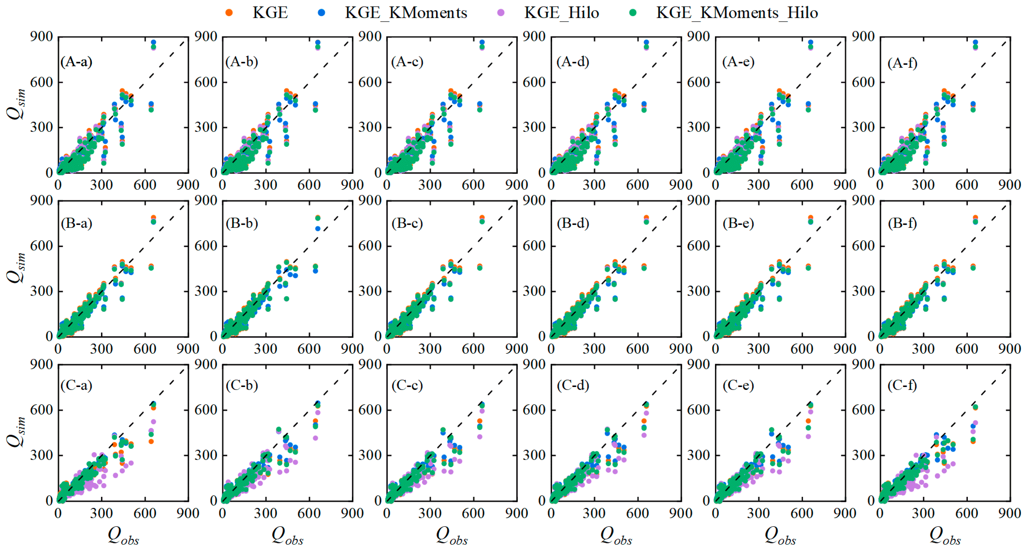
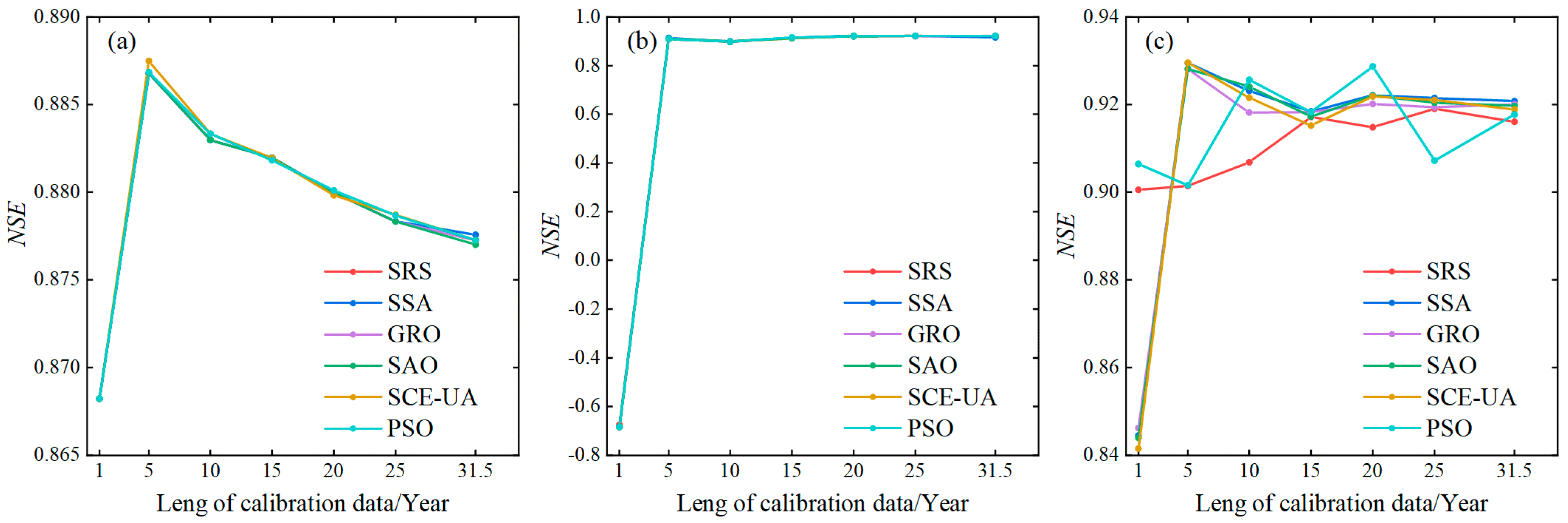
4.2. Comparison of Runoff Modeling Efficiency and Stability

In addition to evaluating the performance of the hydrological models after using the optimization algorithms, another critical concern of the tested optimization algorithms is stability and time consumption. According to the conclusions on the goodness of the four objective functions in Section 4.1, KGE_KMoments with the best performance is selected as the subsequent objective function to test the stability and time consumption of six optimization algorithms through 50 runs.
Figure 6 shows the boxplots of the NSE and RMSE for validation with the TWBM, abcd and HYMOD models under KGE_KMoments as the objective function. Like the results reported in Section 4.1, the performance of the abcd model is best, followed by the HYMOD and TWBM models. Except for the SSA and SAO algorithms, the others can obtain a relatively stable and acceptable NSE and RMSE in TWBM and abcd model calibration. Despite the slight difference in the mean of NSE and RMSE obtained in the HYMOD model calibrations, the stability of the six algorithms has altered. The NSE and RMSE obtained in the SSA algorithm fluctuate slightly around the mean, while others show relatively poor stability, especially the NSE maximum variation in the SRS algorithm up to 1.6%. Considering that the complexity of TWBM, abcd, and HYMOD model structures increase in turn and the SSA algorithm is mainly used in the parameter calibration of machine learning with good performance [64,65], it can be inferred that the SSA algorithm has strong robustness compared with others for the complex structure of model calibration.
To further assess the stability of the six algorithms, as shown in Figure 7, the distribution of the parameter calibration for 50 iterations of each of the six algorithms was calculated. For the TWBM and abcd models, the parameters determined by the SRS and SCE-UA algorithms have the smallest fluctuation, followed by the GRO and PSO algorithms, while the largest fluctuation of the parameter is the SSA and SAO algorithms, mainly reflected in parameter d of the abcd model. For the HYMOD model, only the parameters Cmax and Rs have relatively good stability under other algorithms, except SRS and GRO, and the other parameters vary greatly within feasible regions. Combining the performance of the models, the above parameter calibration results prove that there are obvious phenomena of “equifinality” [66] in the abcd and HYMOD models [55,67].
Another concern is the time-consuming nature of the algorithm during model calibration. The time consumption and iterations of the three model calibrations under each algorithm through 50 runs are shown in Table 4. The search rate of each algorithm is equal to the quotient of iterations and time. It can be found that the SRS algorithm has the fastest search rate, followed by PSO, SEC-UA, GRO, and SAO (not used in hydrology and with a slight difference). The SSA algorithm has the slowest search rate. As the complexity of the model structure increases, the search rate of the SRS and PSO algorithms have an increasing and then decreasing trend, while the search rate of the others decreases. The results further prove the effectiveness of SRS in the parameter calibration of hydrological models. However, due to the limitations of the hydrological samples and model types, the conclusion that the GRO and SAO algorithms have poor performance in hydrological model parameter calibration still needs further investigation.
According to the above analysis in Section 4.1 and Section 4.2, the performance ranking of the six algorithms for three models under KGE_KMoments as the objective function is presented in Table 5. The top three algorithms are always SRS, SEC-UA, and PSO, and the overall performance of the GRO, SAO, and SSA algorithms is poor. For the TWBM and abcd models, the ranks of six algorithm performances have no significant difference, namely, SRS, SCE-UA or PSO, GRO, SAO, and SSA algorithms, in turn, while the best performance is PSO, followed by the SRS, SCE-UA, GRO, SAO, and SSA algorithms. Based on the above comprehensive analysis of the calibration results, the overall rank of the six algorithms under KGE_KMoments as the objective function is SRS > PSO > SCE-UA > GRO > SAO > SSA.

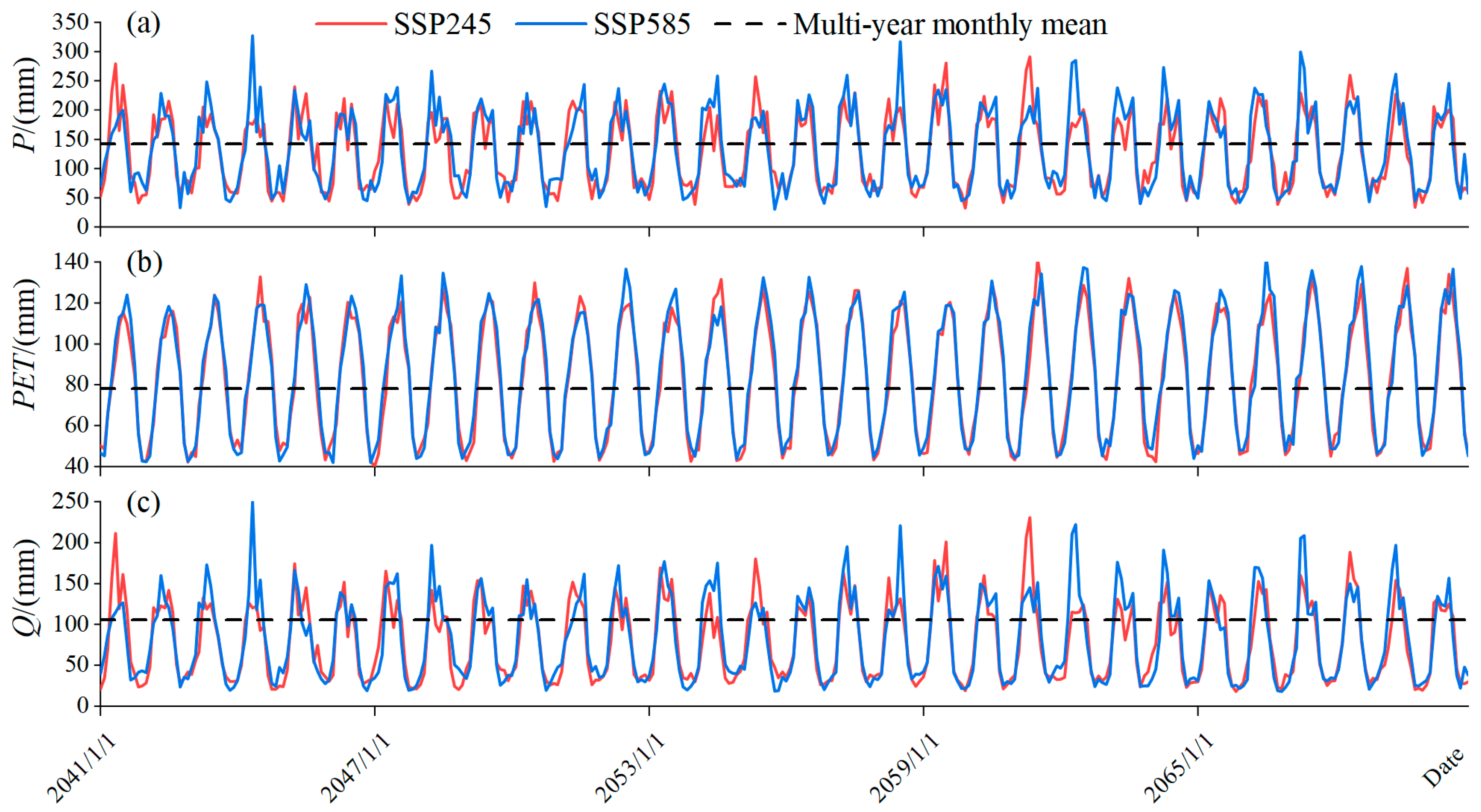
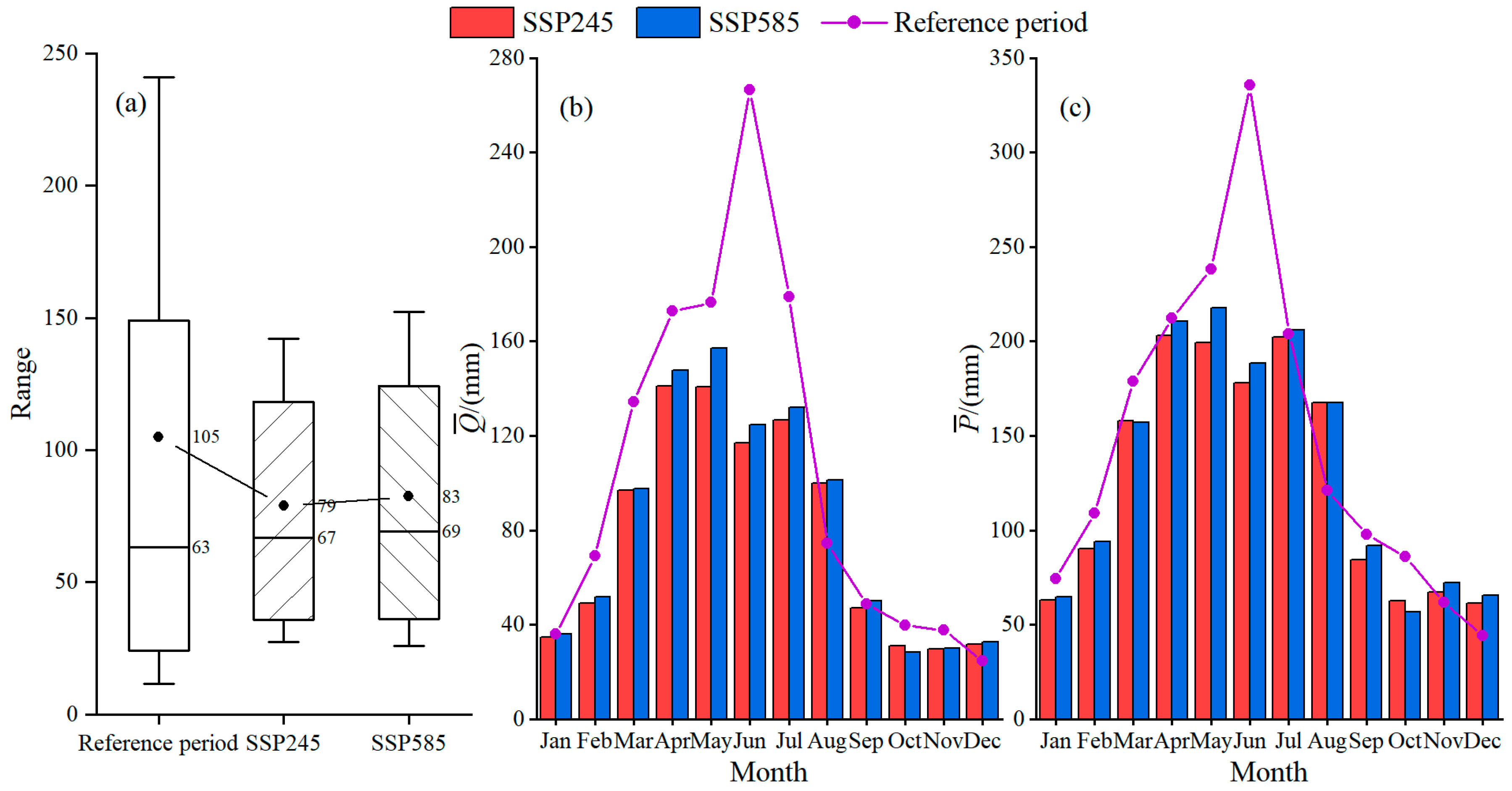
4.3. Runoff Prediction under Future Climate Projections

According to the above results, the abcd model performs best with the NSE equaling 0.913 under the SRS algorithm and KGE_KMoments as the objective function in the validation period. Therefore, the best abcd model was selected to predict and analyze the runoff change under future climate scenarios. The 1971–2000 period is considered the reference period. To reduce the uncertainty caused by the GCM models, the mean ensemble of multiple models is used as the input. Figure 8 shows the change process of hydrological elements including P, PET, and runoff under the SSP245 and SSP585 scenarios. It can be seen that the overall trend of P, PET, and simulated runoff is relatively stable under the influence of climate change, especially for the low value, while the difference between heavy precipitation and high flow is evident. Moreover, the change trends of precipitation and runoff are the same, which proves that precipitation is the dominant factor determining runoff change [68].
Figure 9a lists the box plots of observed streamflow in the reference period and the simulated streamflow for 2041–2070 under the SSP245 and SSP585 scenarios. The mean values of monthly runoff are, respectively, 105 mm, 79 mm, and 83 mm in the reference period for the SSP245 and SSP585 scenarios, which suggests that the simulated runoff will have a significant decreasing trend in 2041–2071 under all SSP scenarios. This also means that the Tunxi catchment may face a certain degree of water shortage in the future. However, compared with the SSP245 scenario, the simulated runoff shows an increasing trend in the SSP585 scenario, which is mainly caused by the increase in rainfall. Figure 9b further demonstrates the intra-annual distribution of runoff under SSP245 and SSP585 scenarios in the future and reference period. It can be found that the distribution of monthly runoff in the Tunxi catchment changed in 2041–2070 under the SSP245 and SSP585 scenarios, with the monthly maximum runoff changing from June to May, and the decrease in the monthly simulated runoff mainly occurring from February to July (10.9–56.1%), while an obvious increase occurred in August and December with an increase of 28.7–36.2%. By further comparing the monthly precipitation in the reference period and the future from Figure 9c, it can be found that the variation trend of precipitation and runoff is highly consistent, which indicates that future precipitation is the dominant factor determining the change in runoff. A similar conclusion was reached in the literature [69] by setting different precipitation scenarios to explore the evolvement mechanism of runoff under climate change and the interaction impacts in Xin’anjiang basin. Moreover, the runoff increases slightly for most months in the future, with an increase in radiative forcing emissions. In the face of these climate change challenges, it is imperative to enhance multi-sectoral collaboration and the integrated management of water resources; advance water-saving technologies, such as drip irrigation and the fusion of water and fertilizer, through the comprehensive control and holistic development of water resources; safeguard the stability of the economic and ecological system in the river basin with food production at its core; and achieve synergy between conservation and utilization. Guiding the allocation of river basin water resources to areas with high industrial and agricultural productivity will ensure efficient use, continually enhancing resilience in managing river basin water resources amidst climate change.

4.4. Discussion

In our study, the efficiency of four objective functions and six algorithms for three hydrological models was first tested, and KGE_KMoments had the best performance, followed by KGE, KGE_KMoments_HiLo, and KGE_HiLo. However, the performance of the objective function is also affected by basin characteristics and model structure, such as the different results obtained by the objective function with the exponent value of the optimal exponent value applied to the model parameter estimation experiment (MOPEX) basins [70]. This study found that, when combining the performance of the abcd model under KGE_HiLo as the objective function, the HiLo method might still have some potential in model parameter calibration for other basins or hydrological models.
Despite considering three aspects of hydrological model calibration, i.e., objective function, optimization algorithm, and model structure, the effect of the length of calibration data on the reliability of models was ignored in the above analysis. Previous research studies have demonstrated that the different lengths of calibration data can lead to completely different calibration results [71,72]. As a supplement, the model calibration data were simply divided into 1, 5, 10, 15, 20, 25, and 31.5 years, calculated forward from the validation period to calibrate the three models under six algorithms. With the increase in the length of calibration data, the performance of the TWBM model shows an increasing and then a decreasing trend, with the best NSE obtained under the length of calibration data equaling 5, while the abcd model has a relatively stable performance, as shown in Figure 10. Similar results can also be found in the study on the effect of calibration data length on the performance of a conceptual hydrological model [73]. It is noted that the performance of the HYMOD model fluctuates with the increase in the length of calibration data, which could indicate that the request of HYMOD models for the data length is higher than the TWBM and abcd models during the monthly model calibration.
Meanwhile, considering the characteristics of model parameters such as the sensibility in conceptual hydrological model calibration is also a popular way to reduce uncertainty. For example, Gan et al. [74] reported that the number of uncalibrated parameters can be reduced by parameter sensitivity analysis, which can improve the efficiency of parameter calibration and obtain a satisfactory runoff. Moreover, with the development of remote sensing technology, remotely sensed products for different hydrologic variables such as evapotranspiration and soil moisture have been used for model calibration. Recent studies have demonstrated the potential of remotely sensed products compared with observed runoff for hydrological model calibration, particularly in ungauged areas [75,76]. Therefore, it is meaningful to further explore the potential of the optimal combination of the above new methods for hydrological model calibration, especially in areas of frequent flooding.
In terms of the future, the above results reveal a decrease in the monthly runoff compared to the reference period in the Tunxi catchment under all SSP scenarios. However, different models may obtain different results due to model structure. For example, Deng et al. [77] used LSTM-based models to predict the change in runoff of the Ganjiang River catchment and found that the result of the CNN-LSTM model presents an opposite trend compared with other models. The Xin’anjiang model, based on the theory of runoff generation under saturated conditions, performs better in humid areas than in arid and semi-arid areas [75]. In our study, it can be found from Figure 11 that the runoff obtained by the HYMOD model is slightly larger than that of other models under the same scenarios, while the future runoff obtained by all models is a decreasing trend compared with the reference period. Moreover, uncertainties existing in future climate change projections also introduce significant uncertainty in future runoff prediction. Many researchers have tried to minimize the uncertainty by improving downscaling methods [78] and using the model mean as input [79]. With the wide application of machine learning, especially deep learning in hydrology, it is meaningful to explore the coupling deep learning and downscaling method to reduce the uncertainty of future runoff prediction.

5. Conclusions

The calibration of hydrological model parameters is a practical problem in the field of hydrology. In this study, six algorithms, i.e., strategic random search (SRS), sparrow search algorithm (SSA), gold rush optimizer (GRO), snow ablation optimizer (SAO), shuffling complex evolution (SCE-UA), and particle swarm optimization (PSO), and the four objective functions of the Kling–Gupta efficiency (KGE) variant relying on knowable moments (KMoments) and considering high and low flows (HiLo) was selected for the TWBM, abcd, HYMOD model calibration in Tunxi basin, China. The three models under the above algorithms and functions achieved relatively good results in the monthly runoff at Tunxi stations. Then, the efficiency, stability, and time consumption of model calibration under the above algorithms and objective functions were analyzed. Finally, the change in future runoff in the Tunxi catchment area under projected climate changes was analyzed via the optimal hydrological model. The main findings can be summarized as follows:
(a) For the historical period of 1956–2000, the abcd model had the best performance with the mean NSE and RMSE equaling 0.913 and 36.6 m3/s in Tunxi station, followed by the HYMOD and TWBM models.
(b) The best performance of runoff simulation was found for KGE_KMoments as the objective function for three models under the same algorithms, which indicates that considering KMoments based on KGE can play a positive role in model calibration, while the adding the HiLo causes instability. Except for the SSA and SAO algorithms used in the HYMDO model, the others can obtain relatively stable and acceptable NSE and RMSE under KGE_KMoments as the objective function. In terms of time consumption, the SRS algorithm has the fastest search rate, followed by PSO, SEC-UA, GRO, and SAO (not used in hydrology and with a slight difference). Based on the comprehensive analysis of the calibration results, the overall rank of the six algorithms is SRS > PSO > SCE-UA > GRO > SAO > SSA.
(c) In terms of the future, the runoff obtained from the above abcd models shows a decrease in the monthly runoff compared to the reference period in the Tunxi catchment area under all SSP scenarios. Moreover, the distribution of monthly runoff changes from 2041 to 2070, with the monthly maximum runoff changing from June to May, and the decrease in monthly simulated runoff mainly occurring from February to July (10.9–56.1%). However, compared with the SSP245 scenario, the simulated runoff shows an increasing trend in the SSP585 scenario, which is mainly caused by the increase in rainfall.
This study proves the availability of the KMoments method, the SRS, and the algorithms not used in hydrology (GRO and SAO) in hydrological model calibration under changing climate conditions, and reveals that the future runoff of the Tunxi catchment area will show a decreasing trend with climate change, which can provide reference for water resource problems brought about by climate change in this area. However, due to the limitations of hydrological samples and model types, the robustness of the KMoments method and SRS, GRO, and SAO algorithms needs to be further explored in the basin with different hydrometeorological characteristics and other hydrological models, especially for machine learning. Moreover, the results of future runoff prediction using the above models are still limited due to the structure of the hydrological model and uncertainties in climate models. Therefore, it is meaningful to explore the coupling deep learning and downscaling method in reducing the uncertainty of future runoff prediction.

Author Contributions

Conceptualization, B.Y. and Y.G.; methodology, Y.G.; software, B.Y.; validation, B.Y. and E.L.; formal analysis, B.Y.; investigation, Y.G.; resources, Y.X.; data curation, E.L.; writing—original draft preparation, B.Y. and E.L.; writing—review and editing, Y.G. and L.N.; visualization, Y.X.; supervision, Y.G. and L.N.; project administration, B.Y.; funding acquisition, B.Y. and Y.G. All authors have read and agreed to the published version of the manuscript.

Funding

This research was funded by the National Key Research and Development Program of China [Grant number: 2022YFC3202401].

Institutional Review Board Statement

Not applicable.

Informed Consent Statement

Not applicable.

Data Availability Statement

Data are available from the corresponding author upon reasonable request.

Acknowledgments

The anonymous reviewers and the editor are thanked for providing insightful and detailed reviews that greatly improved the manuscript.

Conflicts of Interest

The authors declare no conflicts of interest.

References

  1. IPCC. Climate Change 2021: The Physical Science Basis, Summary for Policymakers; Cambridge University Press: Cambridge, UK, 2021. [Google Scholar]
  2. Pan, Z.; Liu, P.; Gao, S.; Xia, J.; Chen, J.; Cheng, L. Improving hydrological projection performance under contrasting climatic conditions using spatial coherence through a hierarchical Bayesian regression framework. Hydrol. Earth Syst. Sci. 2019, 23, 3405–3421. [Google Scholar] [CrossRef]
  3. Miao, C.; Gou, J.; Fu, B.; Tang, Q.; Duan, Q.; Chen, Z.; Lei, H.; Chen, J.; Guo, J.; Borthwick, A.G.L.; et al. High-quality reconstruction of China’s natural streamflow. Sci. Bull. 2022, 67, 547–556. [Google Scholar] [CrossRef] [PubMed]
  4. Wang, W.-c.; Cheng, Q.; Chau, K.-w.; Hu, H.; Zang, H.-f.; Xu, D.-m. An enhanced monthly runoff time series prediction using extreme learning machine optimized by salp swarm algorithm based on time varying filtering based empirical mode decomposition. J. Hydrol. 2023, 620, 129460. [Google Scholar] [CrossRef]
  5. Beck, H.E.; Vergopolan, N.; Pan, M.; Levizzani, V.; van Dijk, A.I.J.M.; Weedon, G.P.; Brocca, L.; Pappenberger, F.; Huffman, G.J.; Wood, E.F. Global-scale evaluation of 22 precipitation datasets using gauge observations and hydrological modeling. Hydrol. Earth Syst. Sci. 2017, 21, 6201–6217. [Google Scholar] [CrossRef]
  6. Zhang, J.; Wang, D.; Wang, Y.; Xiao, H.; Zeng, M. Runoff Prediction Under Extreme Precipitation and Corresponding Meteorological Conditions. Water Resour. Manag. 2023, 37, 3377–3394. [Google Scholar] [CrossRef]
  7. Refsgaard, J.C.; Stisen, S.; Koch, J. Hydrological process knowledge in catchment modelling—Lessons and perspectives from 60 years development. Hydrol. Process. 2022, 36, e14463. [Google Scholar] [CrossRef]
  8. Wu, H.; Zhang, J.; Bao, Z.; Wang, G.; Wang, W.; Yang, Y.; Wang, J. Runoff Modeling in Ungauged Catchments Using Machine Learning Algorithm-Based Model Parameters Regionalization Methodology. Engineering 2023, 28, 93–104. [Google Scholar] [CrossRef]
  9. Mai, J. Ten strategies towards successful calibration of environmental models. J. Hydrol. 2023, 620, 129414. [Google Scholar] [CrossRef]
  10. Zhang, Q.; Zhou, A.; Jin, Y. RM-MEDA: A Regularity Model-Based Multiobjective Estimation of Distribution Algorithm. IEEE Trans. Evol. Comput. 2008, 12, 41–63. [Google Scholar] [CrossRef]
  11. Konapala, G.; Mishra, A.K.; Wada, Y.; Mann, M.E. Climate change will affect global water availability through compounding changes in seasonal precipitation and evaporation. Nat. Commun. 2020, 11, 3044. [Google Scholar] [CrossRef]
  12. Wang, Q.; Sun, Y.; Guan, Q.; Du, Q.; Zhang, Z.; Zhang, J.; Zhang, E. Exploring future trends of precipitation and runoff in arid regions under different scenarios based on a bias-corrected CMIP6 model. J. Hydrol. 2024, 630, 130666. [Google Scholar] [CrossRef]
  13. Zhang, J.; Ma, S.; Song, Y. Hydrological and water quality simulation and future runoff prediction under CMIP6 scenario in the upstream basin of Miyun Reservoir. J. Water Clim. Chang. 2022, 13, 2505–2530. [Google Scholar] [CrossRef]
  14. Zhao, J.; He, S.; Wang, H. Historical and future runoff changes in the Yangtze River Basin from CMIP6 models constrained by a weighting strategy. Environ. Res. Lett. 2022, 17, 024015. [Google Scholar] [CrossRef]
  15. Lei, Y.; Chen, J.; Xiong, L. A comparison of CMIP5 and CMIP6 climate model projections for hydrological impacts in China. Hydrol. Res. 2023, 54, 330–347. [Google Scholar] [CrossRef]
  16. Vrugt, J.A.; Gupta, H.V.; Bouten, W.; Sorooshian, S. A Shuffled Complex Evolution Metropolis algorithm for optimization and uncertainty assessment of hydrologic model parameters. Water Resour. Res. 2003, 39, 1–14. [Google Scholar] [CrossRef]
  17. Zhang, X.; Srinivasan, R.; Zhao, K.; Liew, M.V. Evaluation of global optimization algorithms for parameter calibration of a computationally intensive hydrologic model. Hydrol. Process. 2009, 23, 430–441. [Google Scholar] [CrossRef]
  18. Wang, Y.; Brubaker, K. Multi-objective model auto-calibration and reduced parameterization: Exploiting gradient-based optimization tool for a hydrologic model. Environ. Model. Softw. 2015, 70, 1–15. [Google Scholar] [CrossRef]
  19. Yan, X.; Niu, B.; Chai, Y.; Zhang, Z.; Zhang, L. An adaptive hydrologic cycle optimization algorithm for numerical optimization and data clustering. Int. J. Intell. Syst. 2022, 37, 6123–6151. [Google Scholar] [CrossRef]
  20. Siddique, N.; Adeli, H. Nature Inspired Computing: An Overview and Some Future Directions. Cogn. Comput. 2015, 7, 706–714. [Google Scholar] [CrossRef]
  21. Sivakumar, B. Nonlinear dynamics and chaos in hydrologic systems: Latest developments and a look forward. Stoch. Environ. Res. Risk Assess. 2009, 23, 1027–1036. [Google Scholar] [CrossRef]
  22. Duan, Q.; Sorooshian, S.; Gupta, V. Effective and efficient global optimization for conceptual rainfall-runoff models. Water Resour. Res. 1992, 28, 1015–1031. [Google Scholar] [CrossRef]
  23. Eberhart, R.; Kennedy, J. A new optimizer using particle swarm theory. In Proceedings of the Sixth International Symposium on Micro Machine and Human Science (MHS’95), Nagoya, Japan, 4–6 October 1995; pp. 39–43. [Google Scholar]
  24. Yang, X.S.; Suash, D. Cuckoo Search via Lévy flights. In Proceedings of the 2009 World Congress on Nature & Biologically Inspired Computing (NaBIC), Coimbatore, India, 9–11 December 2009; pp. 210–214. [Google Scholar]
  25. Xue, J.; Shen, B. A novel swarm intelligence optimization approach: Sparrow search algorithm. Syst. Sci. Control Eng. 2020, 8, 22–34. [Google Scholar] [CrossRef]
  26. Wei, H.; Zhang, Y.; Liu, C.; Huang, Q.; Jia, P.; Xu, Z.; Guo, Y. The Strategic Random Search (SRS)—A new global optimizer for calibrating hydrological models. Environ. Model. Softw. 2024, 172, 105914. [Google Scholar] [CrossRef]
  27. Zolfi, K. Gold rush optimizer: A new population-based metaheuristic algorithm. Oper. Res. Decis. 2023, 33, 113–150. [Google Scholar] [CrossRef]
  28. Deng, L.; Liu, S. Snow ablation optimizer: A novel metaheuristic technique for numerical optimization and engineering design. Expert Syst. Appl. 2023, 225, 120069. [Google Scholar] [CrossRef]
  29. Hunter, J.; Thyer, M.; McInerney, D.; Kavetski, D. Achieving high-quality probabilistic predictions from hydrological models calibrated with a wide range of objective functions. J. Hydrol. 2021, 603, 126578. [Google Scholar] [CrossRef]
  30. Wan, Y.; Chen, J.; Xu, C.-Y.; Xie, P.; Qi, W.; Li, D.; Zhang, S. Performance dependence of multi-model combination methods on hydrological model calibration strategy and ensemble size. J. Hydrol. 2021, 603, 127065. [Google Scholar] [CrossRef]
  31. Confesor Jr, R.B.; Whittaker, G.W. Automatic Calibration of Hydrologic Models With Multi-Objective Evolutionary Algorithm and Pareto Optimization1. J. Am. Water Resour. Assoc. 2007, 43, 981–989. [Google Scholar] [CrossRef]
  32. Nash, J.E.; Sutcliffe, J.V. River flow forecasting through conceptual models part I—A discussion of principles. J. Hydrol. 1970, 10, 282–290. [Google Scholar] [CrossRef]
  33. Gupta, H.V.; Kling, H.; Yilmaz, K.K.; Martinez, G.F. Decomposition of the mean squared error and NSE performance criteria: Implications for improving hydrological modelling. J. Hydrol. 2009, 377, 80–91. [Google Scholar] [CrossRef]
  34. McInerney, D.; Thyer, M.; Kavetski, D.; Lerat, J.; Kuczera, G. Improving probabilistic prediction of daily streamflow by identifying Pareto optimal approaches for modeling heteroscedastic residual errors. Water Resour. Res. 2017, 53, 2199–2239. [Google Scholar] [CrossRef]
  35. Sahraei, S.; Asadzadeh, M.; Unduche, F. Signature-based multi-modelling and multi-objective calibration of hydrologic models: Application in flood forecasting for Canadian Prairies. J. Hydrol. 2020, 588, 125095. [Google Scholar] [CrossRef]
  36. Wu, Y.; Liu, S. A suggestion for computing objective function in model calibration. Ecol. Inform. 2014, 24, 107–111. [Google Scholar] [CrossRef]
  37. Althoff, D.; Rodrigues, L.N. Goodness-of-fit criteria for hydrological models: Model calibration and performance assessment. J. Hydrol. 2021, 600, 126674. [Google Scholar] [CrossRef]
  38. Cortés-Salazar, N.; Vásquez, N.; Mizukami, N.; Mendoza, P.A.; Vargas, X. To what extent does river routing matter in hydrological modeling? Hydrol. Earth Syst. Sci. 2023, 27, 3505–3524. [Google Scholar] [CrossRef]
  39. Zhang, Y.; Shao, Q.; Zhang, S.; Zhai, X.; She, D. Multi-metric calibration of hydrological model to capture overall flow regimes. J. Hydrol. 2016, 539, 525–538. [Google Scholar] [CrossRef]
  40. Koutsoyiannis, D. Knowable moments for high-order stochastic characterization and modelling of hydrological processes. Hydrol. Sci. J. 2019, 64, 19–33. [Google Scholar] [CrossRef]
  41. Pizarro, A.; Jorquera, J. Advancing objective functions in hydrological modelling: Integrating knowable moments for improved simulation accuracy. J. Hydrol. 2024, 634, 131071. [Google Scholar] [CrossRef]
  42. Arsenault, R.; Poulin, A.; Côté, P.; Brissette, F. Comparison of Stochastic Optimization Algorithms in Hydrological Model Calibration. J. Hydrol. Eng. 2014, 19, 1374–1384. [Google Scholar] [CrossRef]
  43. Monteil, C.; Zaoui, F.; Le Moine, N.; Hendrickx, F. Multi-objective calibration by combination of stochastic and gradient-like parameter generation rules—The caRamel algorithm. Hydrol. Earth Syst. Sci. 2020, 24, 3189–3209. [Google Scholar] [CrossRef]
  44. Gou, J.; Miao, C.; Duan, Q.; Tang, Q.; Di, Z.; Liao, W.; Wu, J.; Zhou, R. Sensitivity Analysis-Based Automatic Parameter Calibration of the VIC Model for Streamflow Simulations Over China. Water Resour. Res. 2020, 56, e2019WR025968. [Google Scholar] [CrossRef]
  45. Xiong, L.; Guo, S. A two-parameter monthly water balance model and its application. J. Hydrol. 1999, 216, 111–123. [Google Scholar] [CrossRef]
  46. Wang, W.; Li, C.; Xing, W.; Fu, J. Projecting the potential evapotranspiration by coupling different formulations and input data reliabilities: The possible uncertainty source for climate change impacts on hydrological regime. J. Hydrol. 2017, 555, 298–313. [Google Scholar] [CrossRef]
  47. Ávila, L.; Silveira, R.; Campos, A.; Rogiski, N.; Freitas, C.; Aver, C.; Fan, F. Seasonal Streamflow Forecast in the Tocantins River Basin, Brazil: An Evaluation of ECMWF-SEAS5 with Multiple Conceptual Hydrological Models. Water 2023, 15, 1695. [Google Scholar] [CrossRef]
  48. Jam-Jalloh, S.U.; Liu, J.; Wang, Y.; Li, Z.; Jabati, N.-M.S. Wavelet Analysis and the Information Cost Function Index for Selection of Calibration Events for Flood Simulation. Water 2023, 15, 2035. [Google Scholar] [CrossRef]
  49. Sun, J.; Yan, H.; Bao, Z.; Wang, G. Investigating Impacts of Climate Change on Runoff from the Qinhuai River by Using the SWAT Model and CMIP6 Scenarios. Water 2022, 14, 1778. [Google Scholar] [CrossRef]
  50. Zhou, J.; Lu, H.; Yang, K.; Jiang, R.; Yang, Y.; Wang, W.; Zhang, X. Projection of China’s future runoff based on the CMIP6 mid-high warming scenarios. Sci. China Earth Sci. 2023, 66, 528–546. [Google Scholar] [CrossRef]
  51. Peng, S.; Ding, Y.; Liu, W.; Li, Z. 1 km monthly temperature and precipitation dataset for China from 1901 to 2017. Earth Syst. Sci. Data 2019, 11, 1931–1946. [Google Scholar] [CrossRef]
  52. Peng, S. 1-km Monthly Precipitation Dataset for CHINA (1901–2022); National Tibetan Plateau/Third Pole Environment Data Center: Beijing, China, 2020. [Google Scholar] [CrossRef]
  53. Peng, S. 1 km Monthly Potential Evapotranspiration Dataset in CHINA (1901–2022); National Tibetan Plateau/Third Pole Environment Data Center: Beijing, China, 2022. [Google Scholar] [CrossRef]
  54. Wang, W.; Shao, Q.; Yang, T.; Peng, S.; Yu, Z.; Taylor, J.; Xing, W.; Zhao, C.; Sun, F. Changes in daily temperature and precipitation extremes in the Yellow River Basin, China. Stoch. Environ. Res. Risk Assess. 2013, 27, 401–421. [Google Scholar] [CrossRef]
  55. Martinez, G.F.; Gupta, H.V. Toward improved identification of hydrological models: A diagnostic evaluation of the “abcd” monthly water balance model for the conterminous United States. Water Resour. Res. 2010, 46, W08507. [Google Scholar] [CrossRef]
  56. Moore, R.J. The PDM rainfall-runoff model. Hydrol. Earth Syst. Sci. 2007, 11, 483–499. [Google Scholar] [CrossRef]
  57. Moradkhani, H.; Hsu, K.-L.; Gupta, H.; Sorooshian, S. Uncertainty assessment of hydrologic model states and parameters: Sequential data assimilation using the particle filter. Water Resour. Res. 2005, 41, W05012. [Google Scholar] [CrossRef]
  58. Wang, Q.; Yue, C.; Li, X.; Liao, P.; Li, X. Enhancing robustness of monthly streamflow forecasting model using embedded-feature selection algorithm based on improved gray wolf optimizer. J. Hydrol. 2023, 617, 128995. [Google Scholar] [CrossRef]
  59. Xu, D.-m.; Hu, X.-x.; Wang, W.-c.; Chau, K.-w.; Zang, H.-f.; Wang, J. A new hybrid model for monthly runoff prediction using ELMAN neural network based on decomposition-integration structure with local error correction method. Expert Syst. Appl. 2024, 238, 121719. [Google Scholar] [CrossRef]
  60. Khakbaz, B.; Imam, B.; Hsu, K.; Sorooshian, S. From lumped to distributed via semi-distributed: Calibration strategies for semi-distributed hydrologic models. J. Hydrol. 2012, 418, 61–77. [Google Scholar] [CrossRef]
  61. Bazargan, J.; Norouzi, H. Investigation the Effect of Using Variable Values for the Parameters of the Linear Muskingum Method Using the Particle Swarm Algorithm (PSO). Water Resour. Manag. 2018, 32, 4763–4777. [Google Scholar] [CrossRef]
  62. Deng, C.; Zou, J.; Wang, W. Assimilation of remotely sensed evapotranspiration products for streamflow simulation based on the CAMELS data sets. J. Hydrol. 2024, 629, 130574. [Google Scholar] [CrossRef]
  63. Pan, Z.; Deng, C.; Wang, W.; Song, C.; Yang, F. Simulating Runoff and Actual Evapotranspiration via Time-Variant Parameter Method: The Effects of Hydrological Model Structures. J. Hydrol. Eng. 2022, 27, 05022020. [Google Scholar] [CrossRef]
  64. Zhang, X.; Wang, X.; Li, H.; Sun, S.; Liu, F. Monthly runoff prediction based on a coupled VMD-SSA-BiLSTM model. Sci. Rep. 2023, 13, 13149. [Google Scholar] [CrossRef]
  65. Yao, Z.; Wang, Z.; Wang, D.; Wu, J.; Chen, L. An ensemble CNN-LSTM and GRU adaptive weighting model based improved sparrow search algorithm for predicting runoff using historical meteorological and runoff data as input. J. Hydrol. 2023, 625, 129977. [Google Scholar] [CrossRef]
  66. Beven, K. Prophecy, reality and uncertainty in distributed hydrological modelling. Adv. Water Resour. 1993, 16, 41–51. [Google Scholar] [CrossRef]
  67. Bum Kim, K.; Kwon, H.-H.; Han, D. Bias-correction schemes for calibrated flow in a conceptual hydrological model. Hydrol. Res. 2021, 52, 196–211. [Google Scholar] [CrossRef]
  68. Berghuijs, W.R.; Larsen, J.R.; van Emmerik, T.H.M.; Woods, R.A. A Global Assessment of Runoff Sensitivity to Changes in Precipitation, Potential Evaporation, and Other Factors. Water Resour. Res. 2017, 53, 8475–8486. [Google Scholar] [CrossRef]
  69. Zhao, J.; Xu, J.; Cheng, L.; Jin, J.; Li, X.; Chen, N.; Han, D.; Zhong, Y. The evolvement mechanism of hydro-meteorological elements under climate change and the interaction impacts in Xin’anjiang Basin, China. Stoch. Environ. Res. Risk Assess. 2019, 33, 1159–1173. [Google Scholar] [CrossRef]
  70. Tian, F.; Hu, H.; Sun, Y.; Li, H.; Lu, H. Searching for an Optimized Single-objective Function Matching Multiple Objectives with Automatic Calibration of Hydrological Models. Chin. Geogr. Sci. 2019, 29, 934–948. [Google Scholar] [CrossRef]
  71. Motavita, D.F.; Chow, R.; Guthke, A.; Nowak, W. The comprehensive differential split-sample test: A stress-test for hydrological model robustness under climate variability. J. Hydrol. 2019, 573, 501–515. [Google Scholar] [CrossRef]
  72. Ziarh, G.F.; Kim, J.H.; Song, J.Y.; Chung, E.-S. Quantifying Uncertainty in Runoff Simulation According to Multiple Evaluation Metrics and Varying Calibration Data Length. Water 2024, 16, 517. [Google Scholar] [CrossRef]
  73. Ayzel, G.; Heistermann, M. The effect of calibration data length on the performance of a conceptual hydrological model versus LSTM and GRU: A case study for six basins from the CAMELS dataset. Comput. Geosci. 2021, 149, 104708. [Google Scholar] [CrossRef]
  74. Gan, Y.; Liang, X.-Z.; Duan, Q.; Ye, A.; Di, Z.; Hong, Y.; Li, J. A systematic assessment and reduction of parametric uncertainties for a distributed hydrological model. J. Hydrol. 2018, 564, 697–711. [Google Scholar] [CrossRef]
  75. Zhang, Y.; Chiew, F.H.S.; Liu, C.; Tang, Q.; Xia, J.; Tian, J.; Kong, D.; Li, C. Can Remotely Sensed Actual Evapotranspiration Facilitate Hydrological Prediction in Ungauged Regions Without Runoff Calibration? Water Resour. Res. 2020, 56, e2019WR026236. [Google Scholar] [CrossRef]
  76. Liu, X.; Yang, K.; Ferreira, V.G.; Bai, P. Hydrologic Model Calibration With Remote Sensing Data Products in Global Large Basins. Water Resour. Res. 2022, 58, e2022WR032929. [Google Scholar] [CrossRef]
  77. Deng, C.; Yin, X.; Zou, J.; Wang, M.; Hou, Y. Assessment of the impact of climate change on streamflow of Ganjiang River catchment via LSTM-based models. J. Hydrol. Reg. Stud. 2024, 52, 101716. [Google Scholar] [CrossRef]
  78. Gebrechorkos, S.; Leyland, J.; Slater, L.; Wortmann, M.; Ashworth, P.J.; Bennett, G.L.; Boothroyd, R.; Cloke, H.; Delorme, P.; Griffith, H.; et al. A high-resolution daily global dataset of statistically downscaled CMIP6 models for climate impact analyses. Sci. Data 2023, 10, 611. [Google Scholar] [CrossRef] [PubMed]
  79. Mei, Y.; Zhao, S.-s.; Wang, S.-y.; Xie, X.-q.; Wan, S.-q.; He, W.-p. Influence of anthropogenic forcing on the long-range correlation of air temperature in China. Int. J. Climatol. 2022, 42, 10422–10434. [Google Scholar] [CrossRef]
Figure 1. Location of the Tunxi catchment with hydrological stations.
Sustainability 16 06897 g001
Figure 2. Model structures of the three hydrological models used in this study: (a) TWBM; (b) abcd; and (c) HYMOD models.
Sustainability 16 06897 g002
Figure 3. The objective function, (a) 1-KGE, (b) 1-KGE_KMoments, (c) 1-KGE_HiLo, and (d) 1-KGE_KMoments_HiLo values for (A) TWBM, (B) abcd, and (C) HYMOD models during the calibration period.
Sustainability 16 06897 g003
Figure 4. Radar charts of the evaluation metrics (a) NSE and (b) RMSE for the TWBM, abcd, and HYMOD models under the four objective functions and six optimization algorithms during the validation period. The pink, black, and orange algorithm names represent the TWBM, abcd, and HYMOD models, respectively.
Sustainability 16 06897 g004
Figure 5. Scatter plots depicting simulated and observed runoff under the four objective functions and six optimization algorithms (a) SRS, (b) SSA, (c) GRO, (d) SAO, (e) SCE-UA, and (f) PSO of (A) TWBM, (B) abcd, and (C) HYMOD model calibrations in the validation period.
Sustainability 16 06897 g005
Figure 6. Boxplots of performance metrics for (a,b) TWBM, (c,d) abcd, and (e,f) HYMOD models under six optimization algorithms in the validation period. The top line of the box represents the mean with the value label inside the box. The whiskers represent the 95% quantiles.
Sustainability 16 06897 g006
Figure 7. Distribution of parameter calibration for 50 iterations under the six algorithm scenarios: (a,b) TWBM, (cf) abcd, and (gk) HYMOD models.
Sustainability 16 06897 g007
Figure 8. Change process of hydrological elements: (a) P, (b) PET, and (c) runoff under SSP245 and SSP585 scenarios.
Sustainability 16 06897 g008
Figure 9. Comparison of runoff under different climate scenarios in the future and reference period: (a) box plot of all observed and simulated monthly runoff; (b) intra-annual distribution of runoff; (c) intra-annual distribution of precipitation. In each box, the black line with circle markers represents the mean, and the whiskers extend from the 5% to 95% quantiles. The bottom and top edges indicate the 25 and 75 percentiles, respectively.
Sustainability 16 06897 g009
Figure 10. Change in NSE values of the validation period with an increasing number of contributing calibration years: (a) TWBM, (b) abcd, and (c) HYMOD models.
Sustainability 16 06897 g010
Figure 11. Box plots of simulated runoff obtained by the abcd, HYMOD, and TWBM model in 2041–2070 under SSP245 and SSP585 scenarios. In each box, the black line with circle markers represents the mean, and the whiskers extend from the 5% to 95% quantiles. The bottom and top edges indicate the 25 and 75 percentiles, respectively.
Sustainability 16 06897 g011
Table 1. Description of six GCMs of CMIP6 used in this study.
GCM NameSourceSpatial Resolution (Lon° × Lat°)
CanESM5Canadian Centre for Climate Modelling and Analysis, Canada2.81 × 2.81
FGOALS-g3Institute of Atmospheric Physics, Chinese Academy of Sciences, China2 × 2.25
GFDL-ESM4Geophysical Fluid Dynamics Laboratory, National Oceanic and Atmosphere Administration, USA1.25 × 1
INM-CM5-0Institute of Numerical Mathematics of the Russian Academy of Sciences, Russia2 × 1.5
IPSL-CM6A-LRInstitute Pierre-Simon Laplace, France2.5 × 1.26
MPI-ESM1-2-HRMax Planck Institute for Meteorology, Germany0.94 × 0.94
Table 2. Description and prior ranges of the parameters for the three hydrological models.
ModelParametersDescriptionRange
TWBMCEvapotranspiration parameter (-)0.2–2
SCWater storage capacity (mm)0–4000
abcdaThe propensity of runoff to occur before the soil is fully saturated (-)0–1
bThe water storage capacity of the upper soil zone (mm)100–1000
cThe proportion of soil water recharge to groundwater (-)0–1
dThe groundwater runoff recession constant (mm)0–1
HYMODCmaxMaximum catchment storage capacity (mm)1–1500
BexpDistribution soil moisture capacity (-)0.1–2
aDistribution factor between quick/slow routing reservoirs (-)0–1
RsThe ratio of slow flow reservoir (day−1)0–0.1
RqThe ratio of quick flow reservoir (day−1)0–1
Table 3. The core parameter settings of the six optimization algorithms.
AlgorithmsValues
SRSp = 5; δ = 0.01; other is default
SSASearchAgents = 200; Max_iterations = 40
GROSearchAgents = 200; Max_iterations = 40
SAOSearchAgents = 200; Max_iterations = 40
SCE-UAmaxn = 10,000; kstop = 10; pcento = 0.1; iseed = −1; iniflg = 0; ngs = 6
PSOswarmsize = 200;
Table 4. Time consumption and iterations of three hydrological model calibrations under the six algorithm scenarios.
AlgorithmsTWBM Modelabcd ModelHYMOD Model
Time/sIterationsSearch Rate/s−1Time/sIterationsSearch Rate/s−1Time/sIterationsSearch Rate/s−1
SRS71.5335246.88138.17680949.28518.6342788.25
SSA444.020004.50451.0920004.43285.6520002.58
GRO389.520005.14389.5820005.13580.8920002.85
SAO391.320005.11391.3920005.11700.6620002.89
SCE-UA36.171519.7885.8897111.31774.3714985.24
PSO102.1174717.1161.34227737.12691.65635710.94
Table 5. Ranking of the performance of six algorithms with KGE_KMoments as the objective function.
AlgorithmsRank of TWBM ModelRank of abcd ModelRank of HYMOD Model
EfficiencyStabilitySearch RateTotalEfficiencyStabilitySearch RateTotalEfficiencyStabilitySearch RateTotal
SRS111111114122
SSA134523663665
GRO115411441453
SAO126612553544
SCE-UA112211332232
PSO113311222311
Disclaimer/Publisher’s Note: The statements, opinions and data contained in all publications are solely those of the individual author(s) and contributor(s) and not of MDPI and/or the editor(s). MDPI and/or the editor(s) disclaim responsibility for any injury to people or property resulting from any ideas, methods, instructions or products referred to in the content.

