


A Quantitative Analysis of the Complex Response Relationship between Urban Green Infrastructure (UGI) Structure/Spatial Pattern and Urban Thermal Environment in Shanghai


Abstract
:1. Introduction
2. Materials and Methods
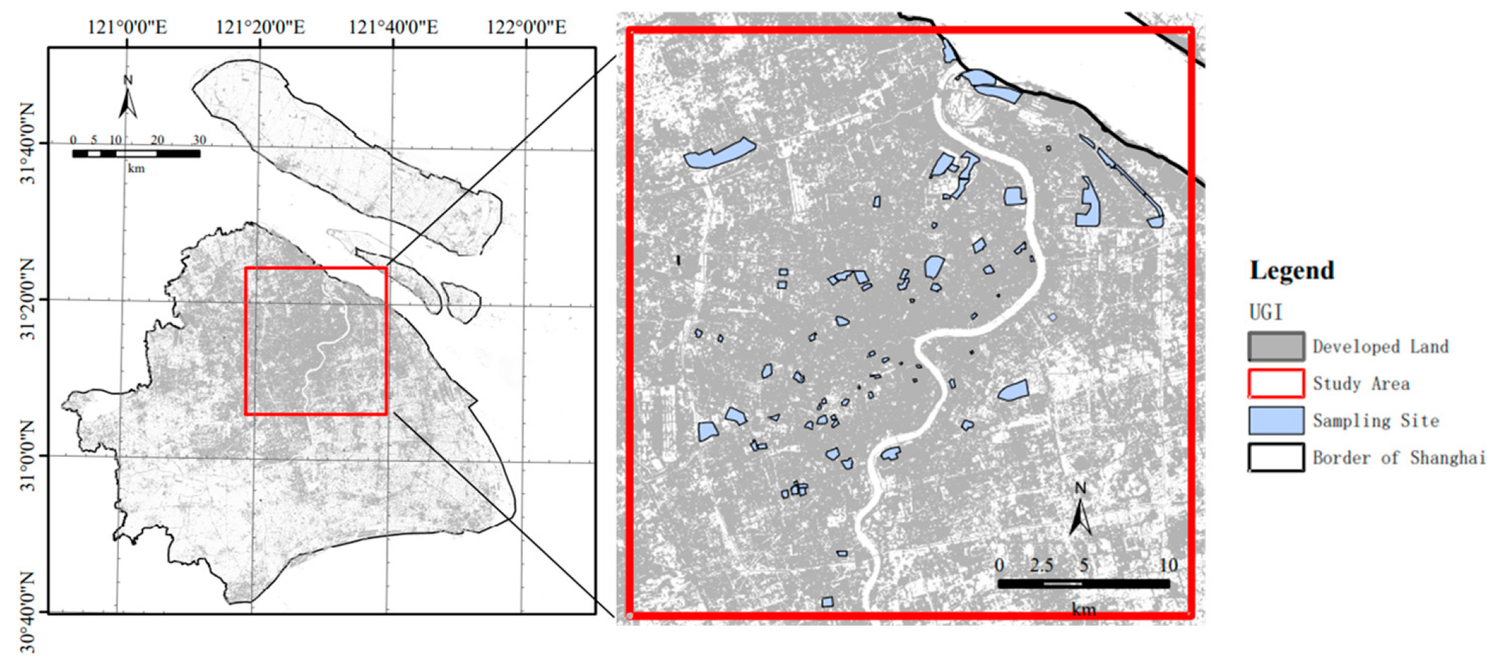
2.1. Study Area
2.2. Data Sources
2.3. Methods
2.3.1. Data Preprocessing
2.3.2. LST Retrieval and Generation of Thermally Sharpened Products
2.3.3. Extraction of Main Variables/Indicators of Built Environment Affecting LST
2.3.4. Statistical Analysis
3. Results
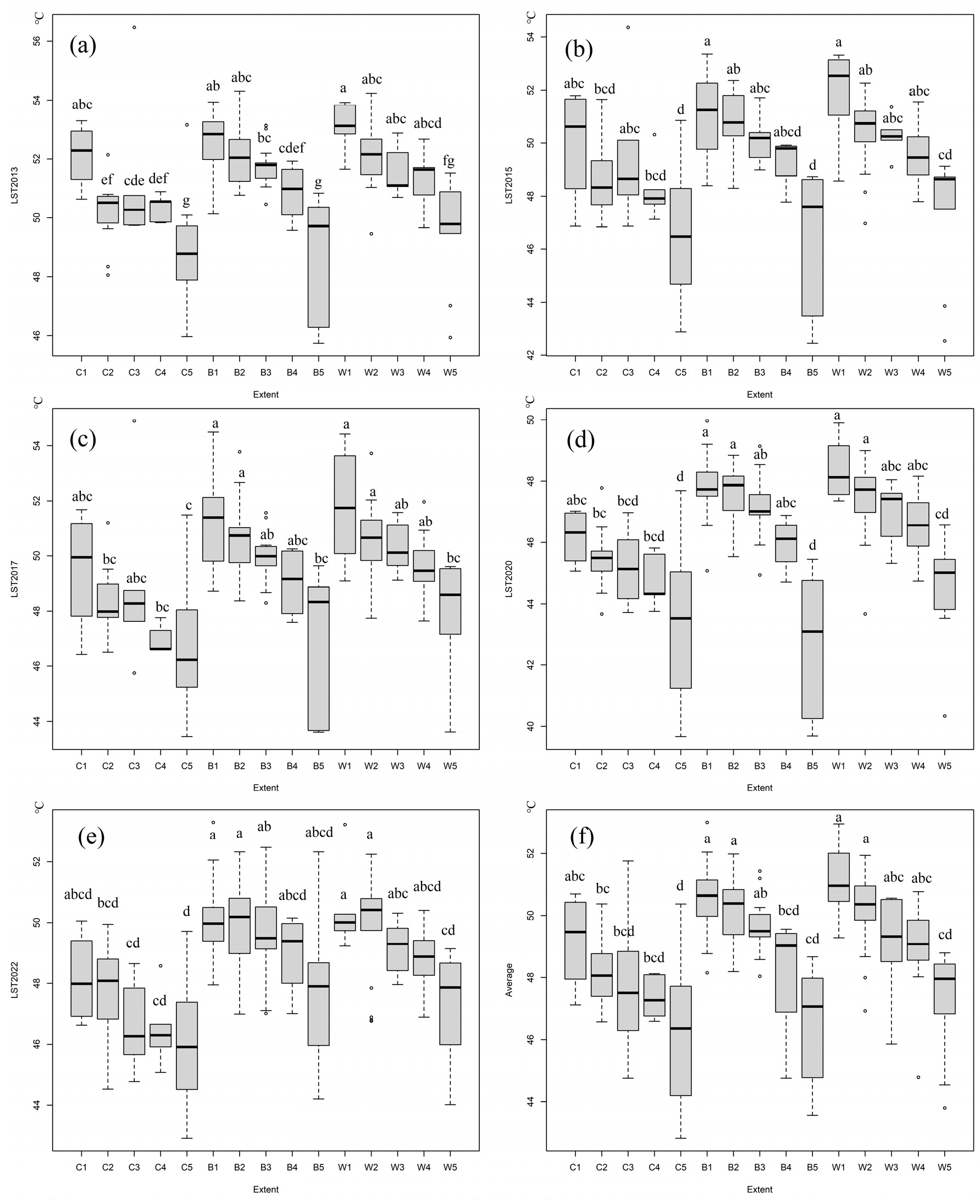
3.1. The Relationship between UGI and LST under Different Spatial Stratification
3.2. Response of LST to UGI Pattern in UTHS Range
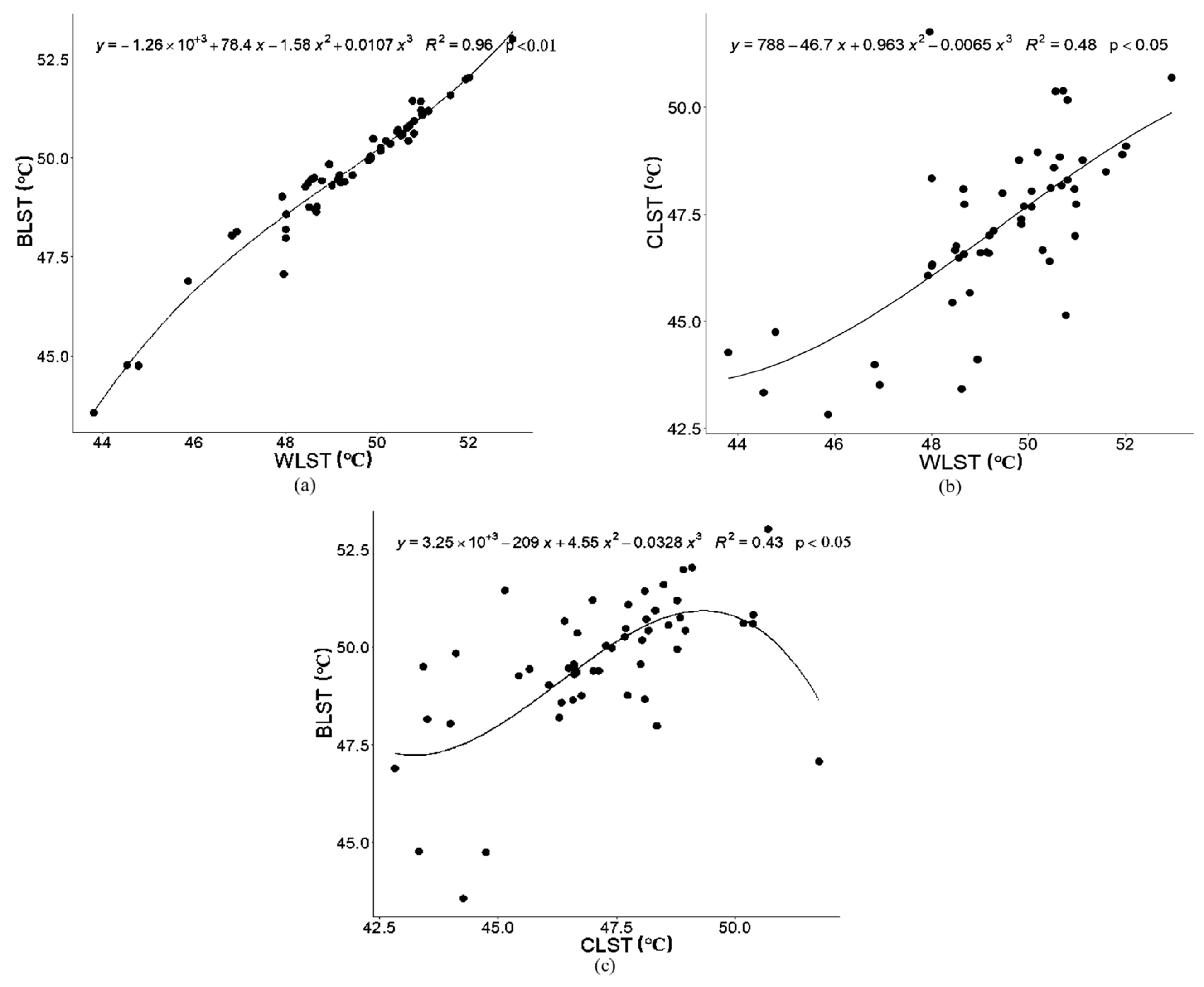
3.3. Quantitative Model Analysis of Pattern Response Relationship between LST and UGI
4. Discussion
4.1. Improving UGI Spatial Pattern to Mitigate UHI Effect
- (1)
- Optimizing three-dimensional greening design. Emphasis is placed on strengthening the optimization of the vertical structure of vegetation and the design of shade so as to effectively increase the vegetation coverage rate in the limited urban greening space. Different types of small green spaces, such as lawns and plants, can be set up on the roofs and external walls of buildings with suitable conditions. On the plane, the greenway system is introduced into urban planning, green belts, tree canopies, and other structures are integrated into the urban landscape, and importance is attached to the role of UGI components in urban management;
- (2)
- Optimizing the layout and management of urban water bodies [74,75,76]. Adapting to local conditions and appropriately increasing small water bodies, mainly with water features such as artificial wetlands, can make good use of the evaporation and heat dissipation effects of water. The rate of rainwater runoff is slowed down by permeable pavements and green lawns, forming large-scale vegetation–water mosaic landscapes, enhancing regional UGI connectivity, lowering urban surface temperatures, and forming a relatively cool microclimate environment.
4.2. Improving Ecological Building Design to Enhance Urban Sustainability
5. Conclusions
Author Contributions
Funding
Institutional Review Board Statement
Informed Consent Statement
Data Availability Statement
Conflicts of Interest
References
- Santamouris, M. Recent progress on urban overheating and heat island research. Integrated assessment of the energy, environmental, vulnerability and health impact. Synergies with the global climate change. Energy Build. 2020; 207, 109482. [Google Scholar]
- Voogt, J.A. Urban heat island: Causes and consequences of global environmental change. In Encyclopaedia of Global Environmental Change; Wiley: Chichester, UK, 2002; Volume 3, pp. 660–666. [Google Scholar]
- Oke, T.R. Boundary Layer Climates; Routledge: London, UK, 2002. [Google Scholar]
- Arnfield, A.J. Two decades of urban climate research: A review of turbulence, exchanges of energy and water, and the urban heat island. Int. J. Climatol. 2003, 23, 1–26. [Google Scholar] [CrossRef]
- Zhao, Z.-Q.; He, B.-J.; Li, L.-G.; Wang, H.-B.; Darko, A. Profile and concentric zonal analysis of relationships between land use/land cover and land surface temperature: Case study of Shenyang, China. Energy Build. 2017, 155, 282–295. [Google Scholar] [CrossRef]
- UN-Habitat. World Cities Report 2022: Envisaging the Future of Cities; UN-Habitat: Nairobi, Kenya, 2022. [Google Scholar]
- Zhao, L.; Lee, X.; Smith, R.B.; Oleson, K. Strong contributions of local background climate to urban heat islands. Nature 2014, 511, 216–219. [Google Scholar] [CrossRef] [PubMed]
- Leal Filho, W.; Echevarria Icaza, L.; Neht, A.; Klavins, M.; Morgan, E.A. Coping with the impacts of urban heat islands. A literature based study on understanding urban heat vulnerability and the need for resilience in cities in a global climate change context. J. Clean. Prod. 2018, 171, 1140–1149. [Google Scholar] [CrossRef]
- Singh, N.; Singh, S.; Mall, R.K. Urban ecology and human health: Implications of urban heat island, air pollution and climate change nexus. In Urban Ecology; Elsevier: Amsterdam, The Netherlands, 2020; pp. 317–334. [Google Scholar]
- Patz, J.A.; Campbell-Lendrum, D.; Holloway, T.; Foley, J.A. Impact of regional climate change on human health. Nature 2005, 438, 310–317. [Google Scholar] [CrossRef]
- Gasparrini, A.; Guo, Y.; Sera, F.; Vicedo-Cabrera, A.M.; Huber, V.; Tong, S.; de Sousa Zanotti Stagliorio Coelho, M.; Nascimento Saldiva, P.H.; Lavigne, E.; Matus Correa, P.; et al. Projections of temperature-related excess mortality under climate change scenarios. Lancet Planet Health 2017, 1, e360–e367. [Google Scholar] [CrossRef] [PubMed]
- Balling, R.C.; Gober, P.; Jones, N. Sensitivity of residential water consumption to variations in climate: An intraurban analysis of Phoenix, Arizona. Water Resour. Res. 2008, 44. [Google Scholar] [CrossRef]
- Wang, C.; Ren, Z.; Guo, Y.; Zhang, P.; Hong, S.; Ma, Z.; Hong, W.; Wang, X. Assessing urban population exposure risk to extreme heat: Patterns, trends, and implications for climate resilience in China (2000–2020). Sustain. Cities Soc. 2024, 103, 105260. [Google Scholar] [CrossRef]
- Buchin, O.; Hoelscher, M.-T.; Meier, F.; Nehls, T.; Ziegler, F. Evaluation of the health-risk reduction potential of countermeasures to urban heat islands. Energy Build. 2016, 114, 27–37. [Google Scholar] [CrossRef]
- Tan, J.; Zheng, Y.; Tang, X.; Guo, C.; Li, L.; Song, G.; Zhen, X.; Yuan, D.; Kalkstein, A.J.; Li, F. The urban heat island and its impact on heat waves and human health in Shanghai. Int. J. Biometeorol. 2010, 54, 75–84. [Google Scholar] [CrossRef]
- Memon, R.A.; Leung, D.Y.; Chunho, L. A review on the generation, determination and mitigation of urban heat island. J. Environ. Sci. (China) 2008, 20, 120–128. [Google Scholar]
- Xu, C.; Chen, G.; Huang, Q.; Su, M.; Rong, Q.; Yue, W.; Haase, D. Can improving the spatial equity of urban green space mitigate the effect of urban heat islands? An empirical study. Sci. Total. Environ. 2022, 841, 156687. [Google Scholar] [CrossRef]
- Wang, Y.; Bakker, F.; de Groot, R.; Wörtche, H. Effect of ecosystem services provided by urban green infrastructure on indoor environment: A literature review. Build. Environ. 2014, 77, 88–100. [Google Scholar] [CrossRef]
- Sun, R.; Xie, W.; Chen, L. A landscape connectivity model to quantify contributions of heat sources and sinks in urban regions. Landsc. Urban Plan. 2018, 178, 43–50. [Google Scholar] [CrossRef]
- Young, R.; Zanders, J.; Lieberknecht, K.; Fassman-Beck, E. A comprehensive typology for mainstreaming urban green infrastructure. J. Hydrol. 2014, 519, 2571–2583. [Google Scholar] [CrossRef]
- Cameron, R.W.F.; Blanuša, T.; Taylor, J.E.; Salisbury, A.; Halstead, A.J.; Henricot, B.; Thompson, K. The domestic garden–Its contribution to urban green infrastructure. Urban For. Urban Green. 2012, 11, 129–137. [Google Scholar] [CrossRef]
- Liu, O.Y.; Russo, A. Assessing the contribution of urban green spaces in green infrastructure strategy planning for urban ecosystem conditions and services. Sustain. Cities Soc 2021, 68. [Google Scholar] [CrossRef]
- Zhang, S.; Muñoz Ramírez, F. Assessing and mapping ecosystem services to support urban green infrastructure: The case of Barcelona, Spain. Cities 2019, 92, 59–70. [Google Scholar] [CrossRef]
- Shen, J.; Peng, Z.; Wang, Y. From GI, UGI to UAGI: Ecosystem service types and indicators of green infrastructure in response to ecological risks and human needs in global metropolitan areas. Cities 2023, 134, 104176. [Google Scholar] [CrossRef]
- Amorim, J.H.; Engardt, M.; Johansson, C.; Ribeiro, I.; Sannebro, M. Regulating and cultural ecosystem services of urban green infrastructure in the nordic countries: A systematic review. Int. J. Environ. Res. Public Health 2021, 18, 1219. [Google Scholar] [CrossRef]
- Kumar, P. The Economics of Ecosystems and Biodiversity: Ecological and Economic Foundations; Routledge: London, UK, 2012. [Google Scholar]
- Maes, J.; Liquete, C.; Teller, A.; Erhard, M.; Paracchini, M.L.; Barredo, J.I.; Grizzetti, B.; Cardoso, A.; Somma, F.; Petersen, J.-E. An indicator framework for assessing ecosystem services in support of the EU Biodiversity Strategy to 2020. Ecosyst. Serv. 2016, 17, 14–23. [Google Scholar] [CrossRef]
- Müller, N.; Kuttler, W.; Barlag, A.-B. Counteracting urban climate change: Adaptation measures and their effect on thermal comfort. Theor. Appl. Climatol. 2013, 115, 243–257. [Google Scholar] [CrossRef]
- Balany, F.; Ng, A.W.M.; Muttil, N.; Muthukumaran, S.; Wong, M.S. Green Infrastructure as an Urban Heat Island Mitigation Strategy—A Review. Water 2020, 12, 3577. [Google Scholar] [CrossRef]
- Hu, L.; Li, Q. Greenspace, bluespace, and their interactive influence on urban thermal environments. Environ. Res. Lett. 2020, 15, 034041. [Google Scholar] [CrossRef]
- Li, F. Planning Green Space for Climate Change Adaptation and Mitigation: A Review of Green Space in the Central City of Beijing. Urban Reg. Plan. 2018, 3. [Google Scholar] [CrossRef]
- Onishi, A.; Cao, X.; Ito, T.; Shi, F.; Imura, H. Evaluating the potential for urban heat-island mitigation by greening parking lots. Urban For. Urban Green. 2010, 9, 323–332. [Google Scholar] [CrossRef]
- Wang, C.; Ren, Z.; Du, Y.; Guo, Y.; Zhang, P.; Wang, G.; Hong, S.; Ma, Z.; Hong, W.; Li, T. Urban vegetation cooling capacity was enhanced under rapid urbanization in China. J. Clean. Prod. 2023, 425, 138906. [Google Scholar] [CrossRef]
- Tan, J.; Zheng, Y.; Song, G.; Kalkstein, L.S.; Kalkstein, A.J.; Tang, X. Heat wave impacts on mortality in Shanghai, 1998 and 2003. Int. J. Biometeorol. 2007, 51, 193–200. [Google Scholar] [CrossRef]
- Zhou, H.; Gao, Y.; Ge, W.; Li, T. The Research on the Relationship Between the Urban Expansion and the Change of the Urban Heat Island Distribution in Shanghai Area. Ecol. Environ. 2008, 17, 163–168. [Google Scholar]
- Zhang, H.; Qi, Z.-f.; Ye, X.-y.; Cai, Y.-b.; Ma, W.-c.; Chen, M.-n. Analysis of land use/land cover change, population shift, and their effects on spatiotemporal patterns of urban heat islands in metropolitan Shanghai, China. Appl. Geogr. 2013, 44, 121–133. [Google Scholar] [CrossRef]
- Li, Y.-y.; Zhang, H.; Kainz, W. Monitoring patterns of urban heat islands of the fast-growing Shanghai metropolis, China: Using time-series of Landsat TM/ETM+ data. Int. J. Appl. Earth Obs. Geoinf. 2012, 19, 127–138. [Google Scholar] [CrossRef]
- Milard, D. Urban Energy and Environmental Policy: The Case of Shanghai since the 2000’s. 2017. Available online: https://www.academia.edu/110727076/Urban_energy_and_environmental_policy_the_case_of_Shanghai_since_the_2000_s (accessed on 1 June 2017).
- Gielen, D.; Chen, C. The CO2 emission reduction benefits of Chinese energy policies and environmental policies: A case study for Shanghai, period 1995–2020. Ecol. Econom. 2001, 39, 257–270. [Google Scholar] [CrossRef]
- Harlan, S.L.; Ruddell, D.M. Climate change and health in cities: Impacts of heat and air pollution and potential co-benefits from mitigation and adaptation. Curr. Opin. Environ. Sustain. 2011, 3, 126–134. [Google Scholar] [CrossRef]
- Shi, C.; Guo, N.; Gao, X.; Wu, F. How carbon emission reduction is going to affect urban resilience. J. Clean. Prod. 2022, 372, 133737. [Google Scholar] [CrossRef]
- Gómez-Baggethun, E.; Barton, D.N. Classifying and valuing ecosystem services for urban planning. Ecol. Econ. 2013, 86, 235–245. [Google Scholar] [CrossRef]
- Shanghai Bureau of Statistics. Shanghai Statistical Yearbook (2021). 2021; p. 2. Available online: https://tjj.sh.gov.cn/tjnj/20220309/0e01088a76754b448de6d608c42dad0f.html (accessed on 1 January 2022).
- Han, J.; Zhao, X.; Zhang, H.; Liu, Y. Analyzing the Spatial Heterogeneity of the Built Environment and Its Impact on the Urban Thermal Environment—Case Study of Downtown Shanghai. Sustainability 2021, 13, 11302. [Google Scholar] [CrossRef]
- Shanghai Municipal Statistics Bureau (SMSB); Survey Office of the National Bureau of Statistics in Shanghai (SONBS-SH). Shanghai Statistical Yearbook-2022; China Statistics Press: Beijing, China, 2021. [Google Scholar]
- Zhang, H.; Han, J.-J.; Zhou, R.; Zhao, A.-L.; Zhao, X.; Kang, M.-Y. Quantifying the relationship between land parcel design attributes and intra-urban surface heat island effect via the estimated sensible heat flux. Urban Clim. 2022, 41, 101030. [Google Scholar] [CrossRef]
- Zhao, M.; Cai, H.; Qiao, Z.; Xu, X. Influence of urban expansion on the urban heat island effect in Shanghai. Int. J. Geogr. Inf. Sci. 2016, 30, 2421–2441. [Google Scholar] [CrossRef]
- Li, J.-j.; Wang, X.-r.; Wang, X.-j.; Ma, W.-c.; Zhang, H. Remote sensing evaluation of urban heat island and its spatial pattern of the Shanghai metropolitan area, China. Ecol. Complex. 2009, 6, 413–420. [Google Scholar] [CrossRef]
- Li, J.; Song, C.; Cao, L.; Zhu, F.; Meng, X.; Wu, J. Impacts of landscape structure on surface urban heat islands: A case study of Shanghai, China. Remote Sens. Environ. 2011, 115, 3249–3263. [Google Scholar] [CrossRef]
- Shanghai Municipal Afforestation Administration. Plan Report for Shanghai Greening System (2002–2020). 2002. Available online: https://www.yuanlin.com/rules/html/detail/2006-4/462.html (accessed on 3 February 2022).
- Zhang, H.; Li, T.t.; Liu, Y.; Han, J.j.; Guo, Y.j. Understanding the contributions of land parcel features to intra-surface urban heat island intensity and magnitude: A study of downtown Shanghai, China. Land Degrad. Dev. 2020, 32, 1353–1367. [Google Scholar] [CrossRef]
- Müller-Wilm, U.; Devignot, O.; Pessiot, L. Sen2Cor Configuration and User Manual. S2-PDGS-MPC-L2A-SUM-V2.4. 2017. Available online: https://step.esa.int/thirdparties/sen2cor/2.4.0/Sen2Cor_240_Documenation_PDF/S2-PDGS-MPC-L2A-SUM-V2.4.0.pdf (accessed on 1 June 2022).
- Feng, L.; Zhao, M.; Zhou, Y.; Zhu, L.; Tian, H. The seasonal and annual impacts of landscape patterns on the urban thermal comfort using Landsat. Ecol. Indic. 2020, 110, 105798. [Google Scholar] [CrossRef]
- Yue, W.; Qiu, S.; Xu, H.; Xu, L.; Zhang, L. Polycentric urban development and urban thermal environment: A case of Hangzhou, China. Landsc. Urban Plan. 2019, 189, 58–70. [Google Scholar] [CrossRef]
- Xu, X.; Liu, Q.; Chen, J. Synchronous retrieval of land surface temperature and emissivity. Sci. China Ser. D Earth Sci. 1998, 41, 658–668. [Google Scholar] [CrossRef]
- Santamouris, M.; Synnefa, A.; Karlessi, T. Using advanced cool materials in the urban built environment to mitigate heat islands and improve thermal comfort conditions. Solar Energy 2011, 85, 3085–3102. [Google Scholar] [CrossRef]
- Næss, P. Built environment, causality and urban planning. Plan. Theory Pract. 2016, 17, 52–71. [Google Scholar] [CrossRef]
- McGarigal, K.; Cushman, S.A.; Ene, E. FRAGSTATS v4: Spatial Pattern Analysis Program for Categorical and Continuous Maps. Computer Software Program Produced by the Authors at the University of Massachusetts Amherst. 2012. Available online: http://www.umass.edu/landeco/research/fragstats/fragstats.html (accessed on 26 July 2018).
- Geladi, P.; Kowalski, B. Partial Least-Squares Regression: A Tutorial. Anal. Chim. Acta 1986, 185, 1–17. [Google Scholar] [CrossRef]
- Wold, H. Soft Modelling by Latent Variables: The Non-Linear Iterative Partial Least Squares (NIPALS) Approach. J. Appl. Probab. 2017, 12, 117–142. [Google Scholar] [CrossRef]
- Wehrens, R.; Mevik, B.-H. The pls package: Principal component and partial least squares regression in R. J. Stat. Softw. 2007, 18, 1–23. [Google Scholar]
- Wu, C.; Li, J.; Wang, C.; Song, C.; Haase, D.; Breuste, J.; Finka, M. Estimating the Cooling Effect of Pocket Green Space in High Density Urban Areas in Shanghai, China. Front. Environ. Sci. 2021, 9, 657969. [Google Scholar] [CrossRef]
- Liu, J.; Zhang, L.; Zhang, Q.; Zhang, G.; Teng, J. Predicting the surface urban heat island intensity of future urban green space development using a multi-scenario simulation. Sustain. Cities Soc. 2021, 66, 102698. [Google Scholar] [CrossRef]
- Jones, L.; Anderson, S.; Læssøe, J.; Banzhaf, E.; Jensen, A.; Bird, D.N.; Miller, J.; Hutchins, M.G.; Yang, J.; Garrett, J.; et al. A typology for urban Green Infrastructure to guide multifunctional planning of nature-based solutions. Nat.-Based Solut. 2022, 2, 100041. [Google Scholar] [CrossRef]
- Adegun, O.B.; Ikudayisi, A.E.; Morakinyo, T.E.; Olusoga, O.O. Urban green infrastructure in Nigeria: A review. Sci. Afr. 2021, 14, e01044. [Google Scholar] [CrossRef]
- Sodoudi, S.; Zhang, H.; Chi, X.; Müller, F.; Li, H. The influence of spatial configuration of green areas on microclimate and thermal comfort. Urban For. Urban Green. 2018, 34, 85–96. [Google Scholar] [CrossRef]
- Lai, D.; Liu, Y.; Liao, M.; Yu, B. Effects of different tree layouts on outdoor thermal comfort of green space in summer Shanghai. Urban Clim. 2023, 47, 101398. [Google Scholar] [CrossRef]
- Yu, K.; Chen, Y.; Wang, D.; Chen, Z.; Gong, A.; Li, J. Study of the Seasonal Effect of Building Shadows on Urban Land Surface Temperatures Based on Remote Sensing Data. Remote Sens. 2019, 11, 497. [Google Scholar] [CrossRef]
- Han, Y.; Taylor, J.E.; Pisello, A.L. Toward mitigating urban heat island effects: Investigating the thermal-energy impact of bio-inspired retro-reflective building envelopes in dense urban settings. Energy Build. 2015, 102, 380–389. [Google Scholar] [CrossRef]
- He, B.-J.; Zhao, Z.-Q.; Shen, L.-D.; Wang, H.-B.; Li, L.-G. An approach to examining performances of cool/hot sources in mitigating/enhancing land surface temperature under different temperature backgrounds based on landsat 8 image. Sustain. Cities Soc. 2019, 44, 416–427. [Google Scholar] [CrossRef]
- He, B.-J. Towards the next generation of green building for urban heat island mitigation: Zero UHI impact building. Sustain. Cities Soc. 2019, 50, 101647. [Google Scholar] [CrossRef]
- Cui, Y.-q.; Zheng, H.-C. Impact of Three-Dimensional Greening of Buildings in Cold Regions in China on Urban Cooling Effect. Procedia Eng. 2016, 169, 297–302. [Google Scholar] [CrossRef]
- Shi, D.; Song, J.; Huang, J.; Zhuang, C.; Guo, R.; Gao, Y. Synergistic cooling effects (SCEs) of urban green-blue spaces on local thermal environment: A case study in Chongqing, China. Sustain. Cities Soc. 2020, 55, 102065. [Google Scholar] [CrossRef]
- Völker, S.; Baumeister, H.; Claßen, T.; Hornberg, C.; Kistemann, T. Evidence for the temperature-mitigating capacity of urban blue space—A health geographic perspective. Erdkunde 2013, 67, 355–371. [Google Scholar] [CrossRef]
- Georgescu, M.; Morefield, P.E.; Bierwagen, B.G.; Weaver, C.P. Urban adaptation can roll back warming of emerging megapolitan regions. Proc. Natl. Acad. Sci. USA 2014, 111, 2909–2914. [Google Scholar] [CrossRef] [PubMed]
- Tian, Y.; Zhou, W. The effect of urban 2D and 3D morphology on air temperature in residential neighborhoods. Landsc. Ecol. 2019, 34, 1161–1178. [Google Scholar] [CrossRef]
- Javadi, R.; Nasrollahi, N. Urban green space and health: The role of thermal comfort on the health benefits from the urban green space; a review study. Build. Environ. 2021, 202, 108039. [Google Scholar] [CrossRef]
- Oliveira, S.; Andrade, H.; Vaz, T. The cooling effect of green spaces as a contribution to the mitigation of urban heat: A case study in Lisbon. Build. Environ. 2011, 46, 2186–2194. [Google Scholar] [CrossRef]
- Theeuwes, N.E.; Steeneveld, G.J.; Ronda, R.J.; Heusinkveld, B.G.; van Hove, L.W.A.; Holtslag, A.A.M. Seasonal dependence of the urban heat island on the street canyon aspect ratio. Q. J. R. Meteorol. Soc. 2014, 140, 2197–2210. [Google Scholar] [CrossRef]
- Park, Y.; Guldmann, J.-M.; Liu, D. Impacts of tree and building shades on the urban heat island: Combining remote sensing, 3D digital city and spatial regression approaches. Comput. Environ. Urban Syst. 2021, 88, 101655. [Google Scholar] [CrossRef]
- Cao, Q.; Liu, Y.; Georgescu, M.; Wu, J. Impacts of landscape changes on local and regional climate: A systematic review. Landsc. Ecol. 2020, 35, 1269–1290. [Google Scholar] [CrossRef]
- Yang, J.; Yang, Y.; Sun, D.; Jin, C.; Xiao, X. Influence of urban morphological characteristics on thermal environment. Sustain. Cities Soc. 2021, 72, 103045. [Google Scholar] [CrossRef]
- Shashua-Bar, L.; Tzamir, Y.; Hoffman, M.E. Thermal effects of building geometry and spacing on the urban canopy layer microclimate in a hot-humid climate in summer. Int. J. Climatol. 2004, 24, 1729–1742. [Google Scholar] [CrossRef]


| Data | Description |
|---|---|
| Landsat-8/9 OLI/TIRS images | Among the available high-quality cloud-free images collected in the summer of 2013–2022, considering the time span and interval of the whole study period, five phases of images were selected in this study: 29 August 2013, 3 August 2015, 24 August 2017, 16 August 2020, and 14 August 2010. These satellite images were downloaded via www.gscloud.cn (accessed on 1 June 2023). |
| Sentinel-1/2 images | Sentinel is a series of Earth observation satellites launched by the Copernicus Program of the European Space Agency (ESA). Three images dated 24 February 2020 16 August 2020, 23 February 2020, and 16 August 2020 were downloaded from the Open port provided by the European Space Agency (https://dataspace.copernicus.eu/browser/?zoom=3&lat=26&lng=0&visualizationUrl=https%3A%2F%2Fsh.dataspace.copernicus.eu%2Fogc%2Fwms%2Fa91f72b5-f393-4320-bc0f-990129bd9e63&datasetId=S2_L2A_CDAS&demSource3D=%22MAPZEN%22&cloudCoverage=30, accessed on 1 June 2023). |
| Land use map | This map of land use cover in 2013 was originally generated using an object-oriented classification method based on orthophose-corrected high-resolution Quickbird satellite imagery. Based on the field investigation data, the classified products were further manually corrected and verified, and resampled to the TIF grid (1 m resolution), with an overall correction accuracy of 91.1% [51]. |
| Building profile data | The building outline is a high-resolution Quickbird satellite image using orthographic correction, and outside the range is manually drawn using the 91 Weitu Map. |
| Digital city thematic products | Commercial thematic layers contain specific land use covers, such as buildings, warehouses, industrial parks, transportation lines, vegetated areas, and bodies of water. (Beijing Digital Space Technology Co., Ltd., Beijing, China) |
| Baidu map | Baidu Maps Baidu web products, including high-resolution satellite images (still/no historical review), thematic features (such as buildings, roads, traffic lines, etc.), and street views with retrospective photos. |
| 91Weitu Map | The online high-resolution satellite image and city digital thematic service layer products operated by Beijing Qianfan World View Company (https://www.91weitu.com, accessed on 20 June 2023). |
| Tianditu map | operated by the National Platform for Common Geospatial Information Services (https://vgimap.tianditu.gov.cn/, accessed on 20 June 2023) |
| Ground truth data | Collected in 8 annual field surveys conducted between 2013 and 2020, with intervals of 3–6 months, focusing on the land use type and development pattern of each typical sample area, building height was measured on-site using the Edkors™ model AS1000H handheld height finder (Changzhou Edkors Instrument Co., LTD, Changzhou, China) . |
| Dimension | Indicator Name | Formula | Meaning |
|---|---|---|---|
| Building index | Proportion of impervious surface area | The proportion of surfaces in a given area that are artificially constructed or artificially enclosed by buildings, roads, sidewalks, etc. | |
| Building height (BH) | / | The vertical height of a building usually indicates the distance from the outdoor floor to the roof of the building. | |
| UGI index | Class area (CA) | It can directly reflect the size of different landscape element types. | |
| percentage of landscape (PLAND) | The relative percentage of a certain patch type in the total landscape area can be used to judge landscape dominance. | ||
| largest patch index (LPI) | The maximum continuous patch area as a percentage of the entire landscape area. | ||
| patch density (PD) | It reflects the degree of fragmentation and spatial heterogeneity of landscape segmentation. | ||
| CLUMPY | It reflects the aggregation and dispersion of patches in the landscape, and the value is between −1 and 1. | ||
| COHESION | Represents the distance and arrangement pattern of patches in the landscape, reflecting the continuity. | ||
| Aggregation Index (Al) | AI ∈ (0,100). AI examined the connectivity between patches of each landscape type. | ||
| Splitting Index (SPLIT) | SPLIT is the sum of the square of the total landscape area divided by the square of the patch area. | ||
| Landscape Shape Index (LSI) | Reflects the complexity of landscape structure; that is, the larger the value, the more complex the shape. |
| Type | Whole Area = Core Area + Buffer Zone | Core Area | Buffer Area | ||||||
|---|---|---|---|---|---|---|---|---|---|
| Impervious Surface Area (%) | Building Area (%) | UGI Area (%) | Impervious Surface Area (%) | Building Area (%) | UGI Area (%) | Impervious Surface Area (%) | Building Area (%) | UGI Area (%) | |
| C1 | 98.95 ± 0.91 | 34.62 ± 10.97 | 1.05 ± 0.91 | 98.28 ± 1.18 | 21.2 ± 5.39 | 1.72 ± 1.18 | 98.98 ± 0.89 | 35.05 ± 11.03 | 1.02 ± 0.89 |
| C2 | 93.20 ± 4.58 | 24.86 ± 9.60 | 6.80 ± 4.58 | 72.03 ± 13.52 | 12.8 ± 8.38 | 25.82 ± 15.16 | 94.62 ± 4.91 | 27.72 ± 7.43 | 5.38 ± 4.91 |
| C3 | 89.83 ± 8.29 | 23.22 ± 8.22 | 10.17 ± 8.29 | 85.73 ± 7.58 | 16.1 ± 4.78 | 14.27 ± 7.58 | 89.63 ± 10.48 | 23.38 ± 9.15 | 10.37 ± 10.48 |
| C4 | 93.75 ± 3.29 | 21.30 ± 3.23 | 6.25 ± 3.29 | 91.84 ± 3.59 | 16.6 ± 4.55 | 8.16 ± 3.59 | 93.98 ± 3.26 | 21.73 ± 3.18 | 6.02 ± 3.26 |
| C5 | 83.78 ± 15.02 | 19.27 ± 8.15 | 15.54 ± 14.93 | 53.88 ± 14.60 | 6.22 ± 6.48 | 52.27 ± 13.85 | 88.27 ± 15.01 | 21.28 ± 7.75 | 11.20 ± 14.93 |
| Entirety | 89.14 ± 11.73 | 22.61 ± 9.20 | 10.56 ± 11.54 | 69.51 ± 20.05 | 11.3 ± 8.20 | 32.64 ± 8.20 | 91.51 ± 11.30 | 24.36 ± 8.56 | 8.26 ± 11.19 |
| 2022 | 2020 | |||||||||
| Coef | S − Coef | T | p | VIF | Coef | S − Coef | T | p | VIF | |
| Constant | 49.145 | 0.443 | 110.953 | 0.000 | 45.634 | 1.364 | 33.465 | 0.000 | ||
| CA | − | − | − | − | − | −5.452 | 0.989 | −5.515 | 0.000 | 3.152 |
| IS | 0.000 | 0.000 | 12.289 | 0.000 | 1.348 | 0.000 | 0.000 | 9.747 | 0.000 | 8.184 |
| PD | − | − | − | − | − | 0.407 | 0.165 | 2.463 | 0.015 | 1.616 |
| LPI | − | − | − | − | − | −0.642 | 0.217 | −2.961 | 0.004 | 16.625 |
| Cohesion | − | − | − | − | − | 0.000 | 0.000 | 5.176 | 0.000 | 20.986 |
| Height | −0.903 | 0.114 | −7.949 | 0.000 | 1.300 | −0.647 | 0.102 | −6.356 | 0.000 | 1.583 |
| SPLIT | 0.000 | 0.000 | 2.067 | 0.040 | 1.042 | − | − | − | − | − |
| S | 1.48198 | 1.20508 | ||||||||
| R-sq | 53.94% | 74.14% | ||||||||
| R-sq(adj) | 53.02% | 73.08% | ||||||||
| R-sq(pred) | 51.53% | 70.40% | ||||||||
| 2017 | 2015 | |||||||||
| Coef | S − Coef | T | p | VIF | Coef | S − Coef | T | p | VIF | |
| Constant | 50.947 | 1.232 | 41.353 | 0.000 | 51.06 | 1.57 | 32.61 | 0.000 | ||
| CA | −5.052 | 1.128 | −4.480 | 0.000 | 3.264 | −6.53 | 1.14 | −5.75 | 0.000 | 3.15 |
| IS | 0.000 | 0.000 | 8.856 | 0.000 | 7.916 | 0.000 | 0.000 | 9.39 | 0.000 | 8.18 |
| PD | − | − | − | − | − | 0.387 | 0.190 | 2.04 | 0.043 | 1.62 |
| LPI | −0.428 | 0.235 | −1.822 | 0.070 | 15.508 | −0.396 | 0.249 | −1.59 | 0.114 | 16.63 |
| Cohesion | 0.000 | 0.000 | 4.584 | 0.000 | 15.968 | 0.000 | 0.000 | 4.15 | 0.000 | 20.99 |
| Height | −0.855 | 0.113 | −7.575 | 0.000 | 1.545 | −0.920 | 0.117 | −7.87 | 0.000 | 1.58 |
| SPLIT | 0.000 | 0.000 | 1.774 | 0.078 | 1.175 | − | − | − | − | − |
| S | 1.35071 | 1.38388 | ||||||||
| R-sq | 69.24% | 70.63% | ||||||||
| R-sq(adj) | 67.98% | 69.43% | ||||||||
| R-sq(pred) | 63.08% | 66.30% | ||||||||
| 2013 | ||||||||||
| Coef | S − Coef | T | p | Coef | ||||||
| Constant | 49.731 | 0.788 | 63.15 | 0.000 | ||||||
| CA | −1.923 | 0.674 | −2.85 | 0.005 | 2.04 | |||||
| IS | 0.000 | 0.000 | 12.36 | 0.000 | 5.27 | |||||
| PD | − | − | − | − | − | |||||
| LPI | − | − | − | − | − | |||||
| Cohesion | 0.000 | 0.000 | 3.53 | 0.001 | 7.04 | |||||
| Height | −0.4381 | 0.079 | −5.54 | 0.000 | 1.32 | |||||
| SPLIT | − | − | − | − | − | |||||
| S | 1.023 | |||||||||
| R-sq | 72.84% | |||||||||
| R-sq(adj) | 72.11% | |||||||||
| R-sq(pred) | 70.89% | |||||||||
| Effect Term | LST2022 | LST2020 | LST2017 | LST2015 | LST2013 | ||||||
|---|---|---|---|---|---|---|---|---|---|---|---|
| Coef | S − Coef | Coef | S − Coef | Coef | S − Coef | Coef | S − Coef | Coef | S − Coef | ||
| Constant | 51.77 | 49.61 | 53.71 | 55.09 | 53.42 | ||||||
| Main effect | CA | −1.18 | −0.13 | −1.28 | −0.12 | −1.45 | −0.13 | −1.74 | −0.14 | −0.93 | −0.10 |
| IS | 0.17 | 0.16 | 0.17 | 0.18 | 0.13 | ||||||
| PD | 0.11 | 0.05 | 0.12 | 0.04 | 0.13 | 0.05 | 0.16 | 0.05 | 0.09 | 0.04 | |
| PLAND | −0.54 | −0.10 | −0.66 | −0.11 | −0.69 | −0.11 | −0.85 | −0.12 | −0.54 | −0.10 | |
| LPI | −0.05 | −0.04 | −0.09 | −0.06 | −0.08 | −0.05 | −0.10 | −0.06 | −0.09 | −0.07 | |
| Cohesion | 0.02 | −0.02 | −0.04 | ||||||||
| AI | 0.07 | 0.03 | 0.06 | 0.05 | −0.01 | ||||||
| Height | −0.57 | −0.47 | −0.49 | −0.35 | −0.65 | −0.43 | −0.74 | −0.44 | −0.25 | −0.20 | |
| LSI | −0.07 | −0.25 | −0.07 | −0.20 | −0.08 | −0.23 | −0.09 | −0.24 | −0.04 | −0.14 | |
| SPLIT | 0.04 | 0.04 | 0.04 | 0.05 | 0.04 | ||||||
| Interaction | PD × SPLIT × LSI | 0.04 | 0.05 | 0.04 | 0.05 | 0.05 | |||||
| effect | CA × Cohesion × AI × LPI | −0.11 | −0.11 | −0.11 | −0.12 | −0.10 | |||||
| IS × Height | −0.05 | −0.01 | −0.04 | −0.03 | 0.03 | ||||||
| IS × Height × PD × SPLIT × LSI | 0.03 | 0.04 | 0.04 | 0.04 | 0.04 | ||||||
| PLAND × PD × SPLIT × LSI | 0.05 | 0.05 | 0.05 | 0.06 | 0.05 | ||||||
| IS × Height × PLAND | −0.03 | 0.01 | −0.02 | −0.01 | 0.03 | ||||||
| PLAND × CA × Cohesion × AI × LPI | −0.11 | −0.11 | −0.11 | −0.12 | −0.10 | ||||||
| F | 15.77 | 19.33 | 16.67 | 23.81 | 20.72 | ||||||
| R2 | 0.673 | 0.652 | 0.670 | 0.699 | 0.749 | ||||||
| Effect Term | LST2022 | LST2020 | LST2017 | LST2015 | LST2013 | ||||||
|---|---|---|---|---|---|---|---|---|---|---|---|
| Coef | S − Coef | Coef | S − Coef | Coef | S − Coef | Coef | S − Coef | Coef | S − Coef | ||
| Constant | 52.01 | 50.88 | 55.05 | 56.52 | 54.84 | ||||||
| CA | −0.93 | −0.10 | −0.72 | −0.07 | −0.49 | −0.04 | −0.95 | −0.07 | −0.12 | −0.01 | |
| Main effect | IS | 0.26 | 0.36 | 0.42 | 0.39 | 0.39 | |||||
| PD | −0.05 | −0.02 | −0.27 | −0.10 | −0.44 | −0.15 | −0.34 | −0.11 | −0.40 | −0.17 | |
| PLAND | −0.70 | −0.13 | −1.09 | −0.18 | −1.26 | −0.19 | −1.39 | −0.19 | −1.05 | −0.19 | |
| LPI | −0.06 | −0.05 | −0.12 | −0.08 | −0.12 | −0.07 | −0.14 | −0.08 | −0.13 | −0.10 | |
| Cohesion | 0.04 | 0.04 | 0.08 | 0.06 | 0.04 | ||||||
| AI | 0.09 | 0.09 | 0.14 | 0.12 | 0.09 | ||||||
| Height | −0.64 | −0.53 | −0.76 | −0.54 | −0.98 | −0.65 | −1.06 | −0.63 | −0.56 | −0.45 | |
| LSI | −0.07 | −0.24 | −0.08 | −0.23 | −0.09 | −0.26 | −0.11 | −0.27 | −0.05 | −0.18 | |
| SPLIT | 0.02 | 0.04 | 0.03 | 0.03 | 0.04 | ||||||
| PD × SPLIT × LSI | 0.02 | 0.04 | 0.04 | 0.04 | 0.05 | ||||||
| Interaction | CA × Cohesion × AI × LPI | −0.09 | −0.08 | −0.06 | −0.08 | −0.05 | |||||
| effect | IS × Height | −0.02 | 0.03 | 0.02 | 0.02 | 0.07 | |||||
| IS × Height × PD × SPLIT × LSI | 0.01 | 0.03 | 0.03 | 0.03 | 0.04 | ||||||
| PLAND × PD × SPLIT × LSI | 0.03 | 0.05 | 0.05 | 0.05 | 0.06 | ||||||
| IS × Height × PLAND | 0.02 | 0.09 | 0.10 | 0.08 | 0.14 | ||||||
| PLAND × CA × Cohesion × AI × LPI | −0.09 | −0.09 | −0.07 | −0.09 | −0.06 | ||||||
| F | 19.69 | 39.29 | 33.05 | 43.47 | 48.57 | ||||||
| R2 | 0.692 | 0.634 | 0.651 | 0.672 | 0.722 | ||||||
| Effect Term | LST2022 | LST2020 | LST2017 | LST2015 | LST2013 | ||||||
|---|---|---|---|---|---|---|---|---|---|---|---|
| Coef | S − Coef | Coef | S − Coef | Coef | S − Coef | Coef | S − Coef | Coef | S − Coef | ||
| Constant | 52.54 | 47.90 | 52.56 | 51.97 | 51.66 | ||||||
| Main effect | CA | −0.51 | −0.04 | −1.70 | −0.13 | −1.52 | −0.11 | −2.26 | −0.16 | −0.50 | −0.05 |
| IS | 0.47 | 0.73 | 0.71 | 0.75 | 0.63 | ||||||
| PD | −0.23 | −0.08 | 0.03 | 0.01 | −0.18 | −0.06 | 0.15 | 0.05 | −0.09 | −0.04 | |
| PLAND | −0.77 | −0.14 | −0.73 | −0.12 | −0.82 | −0.14 | −0.72 | −0.11 | −0.62 | −0.13 | |
| LPI | −0.09 | −0.07 | −0.01 | −0.01 | 0.03 | 0.03 | −0.02 | −0.02 | |||
| Cohesion | 0.19 | 0.36 | 0.36 | 0.39 | 0.28 | ||||||
| AI | 0.01 | −0.01 | 0.02 | 0.01 | 0.02 | ||||||
| Height | −0.94 | −0.52 | −0.94 | −0.49 | −1.08 | −0.55 | −1.15 | −0.55 | −0.61 | −0.38 | |
| LSI | −0.03 | −0.08 | −0.03 | −0.07 | −0.05 | −0.11 | −0.05 | −0.11 | −0.02 | −0.05 | |
| SPLIT | 0.10 | 0.11 | 0.13 | 0.11 | 0.06 | ||||||
| Interaction | PD × SPLIT × LSI | 0.03 | 0.02 | 0.01 | 0.01 | ||||||
| effect | CA × Cohesion × AI × LPI | −0.11 | −0.10 | −0.09 | −0.11 | −0.10 | |||||
| IS × Height | −0.03 | −0.03 | −0.04 | −0.05 | 0.03 | ||||||
| IS × Height × PD × SPLIT × LSI | −0.01 | −0.06 | −0.04 | −0.04 | −0.02 | ||||||
| PLAND × PD × SPLIT × LSI | 0.03 | 0.02 | 0.04 | 0.04 | 0.04 | ||||||
| IS × Height × PLAND | 0.13 | 0.30 | 0.26 | 0.30 | 0.30 | ||||||
| PLAND × CA × Cohesion × AI × LPI | −0.09 | −0.05 | −0.04 | −0.06 | −0.06 | ||||||
| F | 25.95 | 54.73 | 42.29 | 46.17 | 53.60 | ||||||
| R2 | 0.576 | 0.753 | 0.727 | 0.718 | 0.751 | ||||||
Disclaimer/Publisher’s Note: The statements, opinions and data contained in all publications are solely those of the individual author(s) and contributor(s) and not of MDPI and/or the editor(s). MDPI and/or the editor(s) disclaim responsibility for any injury to people or property resulting from any ideas, methods, instructions or products referred to in the content. |
© 2024 by the authors. Licensee MDPI, Basel, Switzerland. This article is an open access article distributed under the terms and conditions of the Creative Commons Attribution (CC BY) license (https://creativecommons.org/licenses/by/4.0/).
Share and Cite
Guan, Z.; Zhang, H. A Quantitative Analysis of the Complex Response Relationship between Urban Green Infrastructure (UGI) Structure/Spatial Pattern and Urban Thermal Environment in Shanghai. Sustainability 2024, 16, 6886. https://doi.org/10.3390/su16166886
Guan Z, Zhang H. A Quantitative Analysis of the Complex Response Relationship between Urban Green Infrastructure (UGI) Structure/Spatial Pattern and Urban Thermal Environment in Shanghai. Sustainability. 2024; 16(16):6886. https://doi.org/10.3390/su16166886
Chicago/Turabian StyleGuan, Zhenru, and Hao Zhang. 2024. "A Quantitative Analysis of the Complex Response Relationship between Urban Green Infrastructure (UGI) Structure/Spatial Pattern and Urban Thermal Environment in Shanghai" Sustainability 16, no. 16: 6886. https://doi.org/10.3390/su16166886
APA StyleGuan, Z., & Zhang, H. (2024). A Quantitative Analysis of the Complex Response Relationship between Urban Green Infrastructure (UGI) Structure/Spatial Pattern and Urban Thermal Environment in Shanghai. Sustainability, 16(16), 6886. https://doi.org/10.3390/su16166886