Smart-City Policy in China: Opportunities for Innovation and Challenges to Sustainable Development

Abstract

Urban development relies on the promotion of innovation, while sustainable development is an inevitable requirement for green urban development. As the primary carrier of innovation and sustainable development, cities have seen the construction of smart cities become a hotspot topic of public concern against the backdrop of rapid advancements in information technology. Based on the Chinese smart-city pilot policies, this paper selects data from 278 prefecture-level cities between 2007 and 2020, employing difference-in-difference (DID), epsilon-based measures and global Malmquist–Luenberger index (EBM-GLM), and the Spatial Durbin Model (SDM) to analyze the direct impact, spatial effects, and regional differences of smart-city construction on urban innovation capacity and sustainable development. The research results indicate the following: (1) the implementation of smart-city policies significantly enhances the urban innovation capacity ($UCI$), but its impact on green total-factor productivity ($GTFP$) is unstable and even insignificant; (2) the $UCI$ and $GTFP$ of smart cities have spillover effects, and the implementation of policies may inhibit the improvement of $UCI$ and $GTFP$ in neighboring cities; (3) the impact of smart-city construction varies across different regions, with a more significant promotion effect on the innovation capacity of economically developed cities.

1. Introduction

The advent of the information age has profoundly changed people’s lifestyles. The emergence of smart products and systems, such as smart furniture, intelligent transportation, intelligent financial management, and smart supervision, has brought great convenience to people’s lives. Some scholars argue that knowledge and the environment have geographical “stickiness”, and innovation and sustainable development also exhibit regional agglomeration effects. This phenomenon is particularly evident at the local city level, thus more effectively promoting urban intelligentization [1]. Therefore, as important carriers of innovation and sustainable development, cities should fully leverage their roles. By strengthening planning, optimizing industrial structures, and improving environmental quality, cities can be developed into livable and workable green spaces, thereby promoting high-quality economic development.

The development of smart cities can be traced back to the mid-1970s. At that time, Los Angeles launched the first large-scale urban data project [2]. Subsequently, various countries formulated smart-city construction policies in the urban dimension to promote the development of smart cities, enhance the convenience of residents’ lives, and improve the living environment. Examples include Barcelona’s Smart City initiative [3], smart cities distributed across North America, South America, Europe, Africa, Oceania, and Asia [4,5,6], smart-city politics in Italy [7], and Australian smart cities [8]. In order to transform the traditional extensive urban development model, the Chinese government launched the National Smart City Policy (SCP) in 2012, which is based on pilot cities, integrating concepts such as “intensive”, “low-carbon”, “ecological”, and “smart” into urban environmental construction. This initiative aims to shape the urban landscape of the Innovation 2.0 era and lead to a city with intelligence bearing Chinese characteristics. Therefore, what is a smart city? What impact does the implementation of smart-city policies have on urban development? These have become hot topics in smart-city research.

Regarding the definition of smart cities, some scholars argue that smart cities are not cities with specific attributes but, rather, a characterization of different contexts within an urban space [9]. Other scholars believe smart cities primarily refer to cities that integrate infrastructure and technological-intermediary services, enhance social learning through human infrastructure, and merge governance through institutional and citizen participation across three dimensions [4]. Concerning the impact of smart-city construction on urban development, existing research has found that smart cities can utilize technology and data to improve the efficiency, economic development, sustainability, and quality of life of urban residents [10]. Additionally, some scholars have utilized the directional distance function (DDF) and Luenberger productivity indicators to measure the green total-factor productivity ($GTFP$) of cities, analyzing the causal relationship between smart-city policies (SCP) and $GTFP$. The results indicate that SCP significantly promotes the $GTFP$ of Chinese cities, mainly through technological innovation, industrial structure upgrading, and resource allocation optimization [11]. Stübinger and Schneider (2020) [12] reviewed the top 200 related research papers ranked by Google Scholar, concluding that intelligence can minimize energy, water, food, waste, heat output, and air pollution and affirming the importance of intelligent, sustainable development in the future. However, most existing studies have focused on the impact of smart-city construction on urban technology, carbon emissions, and $GTFP$ based on DDF–Luenberger. Urban innovation capability is a critical indicator of a city’s future development potential, and green urban development is an essential aspect of sustainable urban development. Currently, there is a lack of research on comprehensive urban innovation capabilities and $GTFP$ based on EBM-GLM. Therefore, this paper systematically explores the impact of smart-city policy implementation on the innovation capabilities and green total-factor productivity of Chinese cities while investigating spatial effects and regional differences.

The marginal contributions of this research are as follows:

• based on the measurement standards for the urban innovation capability index provided in the report “China’s City and Industry Innovation Report 2017” jointly released by the First Financial Research Institute and Fudan University [13] (http://www.360doc.com/content/18/0505/21/26988834_751429774.shtml (accessed on 28 June 2024)), this paper constructs the Urban Innovation Capability Index from two micro-level data: an innovation index (patent maintenance) and an entrepreneurship index (the establishment of enterprises). It then employs the DID and SDM-DID models [14] to analyze both the direct and spatial indirect effects of smart-city construction on urban innovation capability in China.
• Secondly, this paper uses EBM to calculate the city’s green total-factor productivity ($GTFP$). It decomposes $GTFP$ into two parts using GML [15]: the green efficiency change ($GEC$) index and the green technical change ($GTC$) index. From the perspective of urban network externalities, it reassesses the spatial impact of smart cities on urban green total-factor productivity, urban green efficiency change, and urban technological progress using the DID and SDM-DID models, thereby supplementing the academic discussion on issues related to smart-city network externalities.
• Thirdly, this paper categorizes cities based on geographic regions and economic development levels in China, conducts regression on subsamples, and analyzes the regional differences in the impact of smart-city policy implementation on urban innovation capability and urban green total-factor productivity, thus expanding the research perspective on smart cities.

2. Literature Review

With the continuous advancement of information technology, smart cities increasingly represent a significant result of the deep integration of urban modernization and informatization. The existing research has primarily focused on three aspects: the definition of smart cities, the factors influencing the construction of smart cities, and the impact of smart-city construction on urban innovation and urban sustainable development.

2.1. Related Research on the Definition of a Smart City

In the study of smart cities, scholars have engaged in extensive discussions on the question of ”what a smart city is”. However, the definitions of a smart city are varied, and there is currently no unified definition. Nam and Pardo (2011) [4] compiled various interpretations. Hollands (2008) [16] views the smart city as a “city label” phenomenon, particularly in terms of what the label reveals and conceals ideologically. Washburn (2010) [17] defined it as the use of smart computing technologies to make the critical infrastructure components and services of a city—which include city administration, education, healthcare, public safety, real estate, transportation, and utilities—more intelligent, interconnected, and efficient. NRDC (2008) [18] sees a city striving to make itself “smarter” (more efficient, sustainable, equitable, and livable), proposing a definition of “A city that gives inspiration, shares culture, knowledge, and life, a city that motivates its inhabitants to create and flourish in their own lives”. Marsa-Maestre et al. (2008) [19] also believe that smart means more user-friendly than intelligent, as the latter is limited to quick thinking and responding to feedback. A smart city needs to adapt to user needs and provide a customized interface. Therefore, the development of smart cities is multi-faceted. Initially, scholars applied the name to various small dimensions. For example, a digital city [20], an intelligent city [21], an information city [22], a creative city [23], a learning city [24], and so on.

With the advancement of technology, people’s understanding of smart cities has become increasingly comprehensive, and scholars have begun to analyze this concept from more dimensions. Dameri et al. (2013) [25] believe the definition of a smart city is not meant to address a theoretical need but to support the public governance of smart cities by defining visions, goals, and policies that can promote concrete smart implementations. Kim et al. (2017) [26] argue that the main characteristics of a smart city are the high integration of information technology and the comprehensive application of information resources. The fundamental elements of smart-city development include smart technology, smart industry, smart services, smart management, and smart living. Kirimtat et al. (2020) [27] analyzed smart systems from the perspectives of smart people, a smart economy, smart governance, smart mobility, a smart environment, and smart living. Yigitcanlar et al. (2021) [8] argue that innovation, sustainability, and governance are the most popular concepts of smart cities, and the Internet of Things, artificial intelligence, and autonomous vehicle technologies are the most popular technologies.

2.2. Related Research on Factors Influencing Smart-City Construction

Some scholars primarily explore the factors affecting the construction of smart cities from both macro and micro perspectives. On the macro level, urban environmental factors, economic development, structural urban variables, infrastructure, smart-city services, the Internet of Things (IoT), and modern government services are often considered vital factors influencing smart-city development. Neirott et al. (2014) [28] argue that the evolutionary patterns of smart cities (SCs) are highly dependent on local environmental factors. Specifically, economic development and structural urban variables may influence a city’s digital trajectory, geographical location may shape SC strategies, and population density and its associated congestion issues may be crucial components in determining SC implementation pathways. Kim (2022) [29], on the other hand, believes that the construction of urban infrastructure and smart-city services are key factors influencing smart-city development. Rejeb et al. (2022) [30] analyze the main application scenarios of the IoT in smart cities from an IoT perspective, including smart buildings, transportation, healthcare, smart parking, and smart grids. Yaqoob et al. (2023) [31] emphasize the promotion of smart-city construction through factors such as improving infrastructure, modernizing government services, increasing accessibility, accelerating economic growth, and promoting sustainability. Additionally, Alizadeh and Sharifi (2023) [32] consider social justice a critical aspect of smart-city construction. Kruhlov et al. (2024) [33] view the construction of PPP projects as an effective means to promote urban development based on the concept of smart cities.

On the micro level, the analysis focuses on clean technology, information and communication technology (ICT), and governance mechanisms. Lai et al. (2020) [10] believe that clean technology can advance the development of smart cities, including energy, transportation, and sanitation. Chen (2021) [34] states that most components of a smart city rely heavily on ICT. Mora et al. (2023) [35] argue that governance mechanisms are crucial for the transformation of smart cities. However, some scholars contend that many studies have emphasized the benefits of smart cities while neglecting the drawbacks of technology and failed projects, as well as the potential impacts on data privacy and security, which should be given more attention [36,37].

2.3. The Impact of Smart-City Construction on Urban Innovation and Sustainable Development

Cities are the primary carriers of innovation, and sustainable development constitutes a significant component of green cities. Therefore, the existing research has primarily analyzed the impact of smart-city construction on urban innovation and urban sustainable development.

In terms of urban innovation, Bibri and Krogstie (2020) [38] found, by comparing London and Barcelona, two leading data-driven smart cities in Europe, that these cities have a high level of development in applied data-driven technologies. It can thus be inferred that smart-city construction can drive the growth of applied data-driven technologies. Yang et al. (2024) [39], based on micro-enterprise data from the China Taxation Survey Database and the China Innovation Enterprise Database for the period of 2010–2015, found that China’s Smart City Pilot Policy (SCPP) can encourage firm-level green innovation. Additionally, the impact of green innovation on SCPP is more pronounced for non-state-owned enterprises, heavily polluting industries, and non-resource-based city enterprises compared to state-owned enterprises, lightly polluting industries, and resource-based city enterprises. Gohar and Nencioni (2021) [40] and Alahi et al. (2023) [41] argue that smart cities rely on information and communication technology (ICT), and the construction of smart cities can also stimulate the development of urban ICT, such as the construction of 5G communication infrastructure. Kashef et al. (2021) [42] analyzed the demand and impact of smart-city construction on the enhancement of wireless integrated mesh technology (WIMTE) smart-city monitoring systems. Furthermore, scholars have found that smart-city construction helps improve urban innovation performance, although this impact may vary between cities, with each city demonstrating some unique results [43]. Concurrently, the effect of smart-city construction on urban innovation mainly manifests in an increase in innovation activities [44], the enhancement of informatization levels, the strengthening of governmental support for science and technology, the optimization of industrial structures [45], the promotion of green patents [46], green technological innovation, and enterprise innovation [47].

In the field of urban sustainable development, Chu et al. (2021) [48] explored the impact of smart-city construction on the quality of the ecological environment in China. They found that, from 2005 to 2017, China’s smart-city initiatives reduced industrial waste gas and industrial wastewater by approximately 20.7% and 12.2%, respectively. Guo et al. (2022) [43], focusing on China’s smart-city pilot policies, discovered that smart-city construction significantly reduced per-capita CO₂ emissions, with a reduction effect of about 18.42 log points. Moreover, the impact of smart-city construction on CO₂ emission reduction is more notable in cities with higher administrative levels, higher levels of neutral technological progress and green innovation, and more advanced industrial structures.

Meanwhile, Hoang et al. (2021) [49] and Clement et al. (2023) [50] posit that the utilization of renewable energy can reduce pollutant emissions and improve living environment quality. Integrating renewable energy into the energy system of smart cities could achieve more sustainable development. Chen et al. (2022) [51] suggest that energy-saving intelligent street lighting can save substantial energy during peak and off-peak periods, ultimately reducing energy consumption and carbon emissions. Meanwhile, Salman and Hasar (2023) [52] believe that intelligent traffic monitoring and management can reduce urban air pollution.

In addition, Wang et al. (2022) [11] found that SCP policies have a significant positive impact on the green total-factor productivity ($GTFP$) of Chinese cities and exhibit positive spatial spillover effects on the $GTFP$ of adjacent non-pilot cities. However, the spillover effects on neighboring pilot cities are poorer. Nonetheless, Yang et al. (2024) [39] indicate that, in the short term, green innovation in China may exert some adverse effects on green total-factor productivity, but its long-term effects are positive. Additionally, some scholars have found that smart-city construction helps promote innovative urban development and enhance sustainable development and living quality [53], propelling governmental digital governance capabilities and thereby advancing green sustainable development [54].

In addition to researching the impact of smart-city construction on urban innovation and sustainable development, there have also been discussions on other aspects. Sharifi et al. (2021) [55] claim that smart-city initiatives can strengthen resilience against the COVID-19 pandemic and similar future events. Lee et al. (2023) [56] conducted surveys in Amsterdam (the Netherlands), Seoul (South Korea), Portland (USA), and Ho Chi Minh City (Vietnam), concluding that smart-city construction can promote the equity of access to innovative technologies, addressing issues of unfair access and mistrust. Clement et al. (2023) [57] highlight the importance of smart-city strategies in enhancing collaboration between local governments and stakeholders within an ecosystem.

From the above research, it can be seen that, although scholars have analyzed the impact of smart-city construction on urban green total-factor productivity ($GTFP$), their conclusions are inconsistent [11,39]. Additionally, Wang K-L. et al. (2022) [11] primarily used the Luenberger productivity index derived from the directional distance function (DDF) to measure urban $GTFP$. Furthermore, the existing research on the impact of smart cities on urban innovation has mainly been discussed from the perspective of technological innovation, with relatively scant discussion on comprehensive urban innovation capabilities. Therefore, this paper was intended to construct a comprehensive urban innovation capability index based on the microdata of the innovation index and the entrepreneurship index, according to the calculation standards of urban innovation capability in the “China Urban and Industrial Innovation Report 2017” [13]. It employs the EBM-GML method to measure urban $GTFP$, the green efficiency change ($GEC$) index, and the green technical change ($GTC$) index. By adopting a different measurement perspective, this study discusses the impact of smart cities on urban innovation and sustainable development, which can validate existing research conclusions and enrich the analysis of the effects of smart cities.

3. Research Hypotheses, Methods, and Models

3.1. Research Hypotheses

Innovation is the driving force behind urban development, and the city serves as the primary carrier of innovation. The enhancement of a city’s innovation capacity is mainly reflected in two aspects. On the one hand, there is urban infrastructure construction. Existing research indicates that the development of smart cities relies primarily on information and communication technology (ICT). The construction of smart cities can also drive the growth of urban ICT, such as the establishment of 5G communication infrastructure [40,41]. On the other hand, there are advancements and innovations in core urban technologies. Studies have found that smart-city construction can propel the development of data-driven technologies [38], enhance the construction of urban wireless integrated mesh technology (WIMTE) smart-city monitoring systems [42], increase innovative activities [44], improve informatization, strengthen government support for science and technology, and optimize industrial structures [45,58]. It also promotes the increase in green patents [46], green technology innovation, and corporate innovation [47], thereby enhancing urban innovation performance [43].

Moreover, Yang et al. (2024) [39], based on micro-enterprise data from the Chinese Tax Survey Database and the China Innovation Enterprise Database from 2010 to 2015, found that China’s Smart City Pilot Policy (SCPP) can encourage green innovation at the enterprise level. Additionally, some researchers believe smart cities, by utilizing advanced information and communication technologies, have achieved intelligent and refined urban management [59,60]. Furthermore, the data sharing and openness of smart cities also promote the aggregation and sharing of innovation resources, improving the efficiency of innovation resource utilization [61]. This helps enhance urban operational efficiency, optimize resource allocation, and create a more favorable environment for innovative activities. By introducing the next generation of information technologies, smart cities promote a deep integration of traditional industries with information technology, giving rise to new industries, new business forms, and new models. This not only provides a new impetus for urban innovation but also promotes the sustainable development of urban economies. Therefore, this paper’s first null hypothesis (H1_0) and alternative hypothesis (H1_1) are stated as follows:

Null hypothesis (H1_0). 

The implementation of smart-city policies cannot significantly improve urban innovation capabilities.

Alternative hypothesis (H1_1). 

The implementation of smart-city policies can improve urban innovation capabilities.

The construction of smart cities, in addition to influencing urban innovation, has been shown to exert a significant impact on urban sustainable development. This impact is analyzed from both positive and negative perspectives.

Regarding the positive impacts, research has found that smart-city development can reduce the emissions of industrial waste gas and wastewater [48], lower per-capita carbon dioxide emissions [43], increase the use of renewable energy, and reduce pollutant emissions [49,51,57], ultimately improving the quality of the ecological environment. Salman and Hasar (2023) [52] also found that intelligent traffic monitoring and management can reduce urban air pollution. Additionally, researchers have discovered that SCP policies have a significantly positive impact on the green total-factor productivity ($GTFP$) of cities [11]. Smart city development helps promote urban innovation, enhance sustainable development, and improve the quality of life [53]. It also advances governmental digital governance capabilities, thereby promoting green and sustainable development [54].

As for the negative impacts, Yang et al. (2024) [39] indicated that China’s green innovation might have a particular adverse effect on green total-factor productivity in the short term. Simultaneously, the pursuit of innovative development in smart cities might sometimes suppress urban sustainable development due to the neglect of specific issues. These issues include inappropriate technology applications, the energy consumption of data centers, environmental neglect, and data security concerns. In the construction of smart cities, over-reliance on high-energy-consumption technologies or the introduction of technology without fully considering its environmental impact could lead to increased energy consumption and environmental pollution, thus hindering green urban development [62]. Smart cities usually involve extensive data collection, storage, and processing, which typically necessitates the construction of large data centers. Data centers are highly energy-consuming facilities, and if not built and managed correctly, they could become a bottleneck for green urban development [63]. Additionally, in the quest for innovation, if the construction of smart cities neglects socio-environmental impact assessments, it might lead to the implementation of projects or policies detrimental to sustainable development [64]. Furthermore, poor management, a lack of attention to information security, and technological leaks can lead to data security issues such as identity verification, unauthorized access, device-level vulnerabilities, and sustainability [65], resulting in social problems like extremism, polarization, misinformation, and internet addiction [66]. Ismagilova et al. (2020) [67] and Laufs et al. (2020) [68] also asserted that increasing research is focusing on the security, privacy, and risks associated with smart cities, highlighting the threats related to information security and the challenges in managing and processing personal data within smart-city infrastructures. Spicer et al. (2023) [69] used unique survey data from residents of three prominent Canadian cities—Vancouver, Montreal, and Toronto—to study inconsistency between the types of projects pursued by cities, in particular service and policy areas, and the preferences of the residents. However, the calculation of green total-factor productivity mainly includes the input and output sub-components through factoring in energy consumption and environmental issues within the traditional total-factor productivity analysis framework, reflecting the coordination between the economy and the environment. Therefore, combining the above analyses, the impact of smart cities on urban green total-factor productivity might be both positive and negative. Accordingly, this paper’s second null hypothesis (H2_0) and alternative hypothesis (H2_1) are stated as follows:

Null hypothesis (H2_0). 

The impact of smart city policies on urban green total-factor productivity is unstable and may even be insignificant.

Alternative hypothesis (H2_1). 

The impact of smart city policies on urban green total-factor productivity is significantly positive or negative.

The development of cities often exhibits certain network externalities that can have an impact on the development of neighboring cities. Wang et al. (2022) [11] found that SCP had a positive spatial spillover effect on the $GTFP$ of adjacent non-pilot cities, but the spillover effect on adjoining pilot cities was relatively poor. In addition, some studies have found that smart cities provide innovative talents with more convenient work and living environments, attracting a large number of high-end talent and innovation teams [70], which in turn attracts and gathers innovative talent and institutions, promotes the innovation level of the city itself, and creates a siphon effect on the talents of neighboring cities [58]. Due to the connections between various links in the industrial chain, the location choice of enterprises tends to be areas with spatial comparative advantages, thereby actively or passively influencing the innovation capacity and green total-factor productivity of neighboring cities. Therefore, the paper’s third null hypothesis (H3a_0) and alternative hypothesis (H3a_1) are stated as follows:

Null hypothesis (H3a_0). 

The implementation of smart-city policies has no significant spatial effects capable of influencing the innovation capacity and green total-factor productivity of neighboring cities through city network externalities.

Alternative hypothesis (H3a_1). 

The implementation of smart-city policies has spatial effects capable of influencing the innovation capacity and green total-factor productivity of neighboring cities through city network externalities.

Furthermore, apart from city externalities, differences in city development inherently exist. Studies have pointed out that, compared to state-owned enterprises, enterprises in light-pollution industries, and enterprises in non-resource-based cities, the impact of green innovation on SCP is more significant for non-state-owned enterprises, enterprises in heavily polluting industries, and enterprises in non-resource-based cities [39]. Scholars have also found that the construction of smart cities helps enhance urban innovation performance. Still, this effect may vary among different cities, with each city exhibiting some unique outcomes. The impact of smart-city construction on CO₂ emission reductions is more significant in cities with higher administrative levels, higher levels of neutral technological progress and green innovation, and more advanced industrial structures [43]. In this context, a neighboring city is defined as a neighboring city based on its geographical location. If it is neighboring, it is a neighboring city; if not, it is a nonneighboring city. Therefore, this paper’s fourth null hypothesis (H3b_0) and alternative hypothesis (H3b_1) are stated as follows:

Null hypothesis (H3b_0). 

The implementation of smart-city policies causes no significant regional or city differences in influencing urban innovation capacity and green total-factor productivity.

Alternative hypothesis (H3b_1). 

The implementation of smart-city policies causes regional and city differences in influencing urban innovation capacity and green total-factor productivity.

3.2. Selection of Methods and Models

The difference-in-differences (DID) model [14], as one of the primary means of studying the net effects of policies, becomes particularly important when examining the differences in innovation capacity and sustainable development levels between smart pilot cities and non-pilot cities. Considering that the selection and establishment times of smart pilot cities exhibit significant variations across cities nationwide, this variation is further amplified under the influence of policies, thereby increasing the differences in innovation capacity and sustainable development levels between the two types of cities. Therefore, this study treats the designation of smart pilot cities as an approximate natural experiment for in-depth exploration. However, the non-random selection of smart pilot cities may lead to selection bias in the experiment, which could potentially cause endogeneity issues in the sample. The classic econometric model of difference-in-differences (DID) is employed to address the endogeneity issues caused due to selection bias. Since the approvals of smart pilot cities are not concentrated in a single year, this study uses a multi-period DID model for analysis. For multi-period panel data, the model is defined as follows:

$$y_{it}={\beta }_0+{\beta }_{1}DI{D}_{it}+X_{it}\gamma +{\lambda }_i+v_t+{ϵ}_{it}$$

(1)

In which $y_{it}$ represents the i-th city in the j year of the explained variable, which is mainly $UCI$, $GTFP$, $GEC$, or $GTC$ in this paper, respectively; $DI{D}_{it}$ represents the i-th city in the j year of the dummy variable for the smart pilot-city policy; ${\beta }_1$ denotes the policy effect or treatment effect; ${\lambda }_i$ stands for individual fixed effects; $X_{it}$ are the control variables; $v_t$ represents time fixed effects; ${ϵ}_{it}$ is the disturbance term.

In the classical difference-in-differences (DID) method, there is a critical assumption called the “Stable Unit Treatment Value Assumption” (SUTVA). This assumption posits that the potential outcome of each unit should be unique after receiving treatment and not influenced by the treatment of other units [71]. However, in the real spatial dimension, it is challenging to consider each city as a completely independent spatial unit. Particularly when considering the implementation of smart pilot policies, the spatial correlation of these policies and potential spillover effects may render the SUTVA non-applicable in practice [72]. Furthermore, the transmission of spatial effects may be in not only the spatial lag terms of the dependent variable but also the variations in the error terms caused by random shocks [73,74]. Therefore, this study constructed a Difference-in-Differences Spatial Durbin Model (DID-SDM):

$$y_{it}={\beta }_0+{\beta }_{1}DI{D}_{it}+{\delta }_1{W}_n\ast DI{D}_{it}+\rho W_n\ast y_{it}+X_{it}\gamma +{\lambda }_i+v_t+(I-\lambda W_n){ϵ}_{it}$$

(2)

Among them, $W_n$ is an $n\ast n$ spatial weight matrix where each element in the matrix represents the connection between region i and region j. Due to the existence of spillover effects, smart pilot cities may have an impact on neighboring cities, and this average spillover effect is measured by ${\delta }_1$. Therefore, in the case of incorporating spatial spillover effects, the policy effect for the experimental group, and the policy effect for the control group, is ${\delta }_1{W}_n$. The $\rho$ represents the impact of the explained variable of adjacent regions in the defined weight matrix. The other variables are the same as in Formula (1).

The classic difference-in-differences (DID) method requires that the experimental group and the control group satisfy the parallel trend assumption before the policy implementation, showing no significant difference before the policy and significant difference after the policy implementation. That is, the regression coefficients are not significant before the policy implementation, and they become significant after the policy implementation, thereby verifying the difference in the changing trend of the experimental group and the control group before and after the policy implementation. This study adopts the event study methodology of Beck et al. (2010) [75] to construct the parallel trend test model, as shown in the following formula:

$$y_{it}={\alpha }_1+{\beta }_{-5}tim{e}_{it}^{-5}+{\beta }_{-4}tim{e}_{it}^{-4}+\cdots +{\beta }_{5}tim{e}_{it}^5+X_{it}\gamma +{\lambda }_i+v_t+{ϵ}_{it}$$

(3)

Here, in the variable $tim{e}_{it}^n$, where the superscript $n>0$ indicates n years after the baseline year of policy implementation, and $n<0$ indicates n years before the baseline year of policy implementation. ${ϵ}_{it}$ is the random disturbance term. The other variables are the same as in Formula (1).

4. Materials and Study Design

4.1. Materials’ Data and Variables Description

According to the data published by the Ministry of Civil Affairs of the People’s Republic of China, there are a total of 293 prefecture-level cities in China (http://xzqh.mca.gov.cn/map (accessed on 28 June 2024)). However, between 2007 and 2020, with the development of cities, some statistical indicators at the urban scale might be missing. For the convenience of this study, data from 15 prefecture-level cities with substantial missing indicators were removed. (The deleted prefecture-level cities include Tangshan City, Puer City, Tongren City, Bijie City, Danzhou City, Sansha City, Turpan City, Hami City, Haidong City, Lhasa City, Xigaze City, Qamdo City, Nyingchi City, Shannan City, and Naqu City). Ultimately, this study constructed a balanced panel dataset of 278 prefecture-level cities from 2007 to 2020, totaling 3892 samples.

The data required to construct the urban innovation capability index in this study mainly came from two parts of microdata: the number of patents published by the China National Intellectual Property Administration and the registered capital of enterprises from the China State Administration for Industry and Commerce [13]. Meanwhile, the data required to construct the green total-factor productivity index and the control-variable data were primarily sourced from the “China City Statistical Yearbook” (https://www.stats.gov.cn/zs/tjwh/tjkw/tjzl/202302/t20230215_1907995.html (accessed on 28 June 2024)), Wind database (https://www.wind.com.cn/mobile/EDB/zh.html (accessed on 28 June 2024)), EPS database (https://www.epsnet.com.cn/index.html (accessed on 28 June 2024)), statistical yearbooks officially released by provinces, socio-economic statistical bulletins of the provinces, and various databases or web pages of municipal government websites.

For part of the missing data in 2017–2018, interpolation was used to complete the data, ensuring its integrity and accuracy. As a result, a balanced panel dataset was ultimately obtained, including 132 cities that were selected as smart-city pilots and 146 cities that were not selected as smart-city pilots.

4.2. Explained Variables

The dependent variables are the urban innovation capability index ($UCI$) and sustainable development (green total-factor productivity, $GTFP$). The urban innovation capability index ($UCI$) was calculated based on the total-factor productivity, R&D investment, and the number of patents, following the calculation method in the “China Urban and Industrial Innovation Report 2017” [13]. Green total-factor productivity ($GTFP$) was calculated using indicators such as the number of employees in the city district, the built-up area of the city district, the capital stock at the 2006 base period, and the GDP deflator for the 2006 base period. The $GTFP$ was measured from the perspective of input–output to characterize the level of sustainable development in a city. The specific measurement process was as follows: (1) The EBM model proposed by Tone et al. (2010) [76] was used to calculate the environmental efficiency of urban development, which includes undesirable environmental outputs. (2) The GML index was used to decompose the results of the EBM model, yielding the dynamic changes in green total-factor productivity and its decomposition items. The decomposition items mainly include two parts: the green efficiency change ($GEC$) index and the green technical change ($GTC$) index. The green efficiency change index ($GEC$) reflects the impact on resource allocation efficiency due to changes in environmental factors resulting from policy and institutional changes. The green technical change index ($GTC$) refers to the outward shift of the production frontier, driven by technological development. Based on the characteristics of the data, an indicator system for measuring green total-factor productivity was constructed, with output indicators selected as shown in

Table 1. Green total-factor productivity measurement indicator system.

Target Level	Normative Layer		Indicator Layer	Unit
Green total-factor productivity ($GTFP$)	Input indicators	Labor input	Number of persons employed in municipal districts	10,000 people
		Land input	Built-up area of municipal districts	Hm2
		Capital investment	2006 base period capital stock	10,000 yuan (RMB)
	Output indicators	Expected outputs	GDP 2006 base period deflator	10,000 yuan (RMB)
		Indicators of undesired outputs	Sulfur dioxide SO2	t
			Industrial wastewater	wt
			Soot	t

.

4.3. Core Explanatory Variable

This paper primarily investigates the impact of China’s pilot smart-city policies on urban innovation and sustainable development. Therefore, the core explanatory variable of this study is whether a city is included in the pilot smart-city list, denoted as the variable $DID$. The first batch of pilot smart cities in China was established in 2013, so the period from 2007 to 2012 is considered the pre-experiment window for the pilot smart-city policy, and the period from 2013 to 2020 is the experimental period:

(1)

The first batch of smart-city pilot websites in 2012: https://www.mohurd.gov.cn/gongkai/zhengce/zhengcefilelib/201212/20121204_212182.html (accessed on 28 June 2024);

(2)

The second batch of smart-city pilot websites in 2013: https://www.mohurd.gov.cn/gongkai/zhengce/zhengcefilelib/201302/20130205_212789.html (accessed on 28 June 2024);

(3)

The third batch of smart-city pilot websites in 2013: https://www.mohurd.gov.cn/gongkai/zhengce/zhengcefilelib/201308/20130805_214634.html (accessed on 28 June 2024);

(4)

The fourth batch of smart-city pilot websites in 2015: https://www.mohurd.gov.cn/gongkai/zhengce/zhengcefilelib/201504/20150410_220653.html (accessed on 28 June 2024).

The sample of cities approved as pilot smart cities constituted the experimental group, while the other cities formed the control group. During the sample period, prefecture-level cities approved as pilot smart cities were assigned a value of 1 from the year they were approved, i.e., $DID=1$, and 0 before approval, i.e., $DID=0$; other non-pilot smart cities were consistently assigned a value of 0, i.e., $DID=0$. Due to incomplete data for some cities, these were excluded; moreover, some control-group cities were also excluded due to the large number.Therefore, the final study includes 132 pilot smart cities as the experimental-group sample and 146 cities as the control-group sample.

4.4. Control Variables

Based on the existing research literature, the study controlled for urban innovation development and sustainable development by considering three main aspects: macroeconomic development, technological government support, and basic geographical characteristics. Macroeconomic development mainly includes urban per-capita GDP ($pgdp$) and urban employment conditions ($eoye$). Technological government support mainly includes regional government educational expenditure ($edexp$) and regional government scientific and technological expenditure ($sciexp$). The basic geographical characteristics of a city mainly include the urban built-up area ($bua$). In addition, to facilitate the robustness of the analytical conclusions, urban per-capita GDP ($pgdp$), urban employment conditions ($eoye$), and regional government educational expenditure ($edexp$) were substituted with regional gross domestic product ($pdg$), the proportion of the secondary industry in the regional gross domestic product ($sis$), and local general public budget expenditure ($fina$), respectively, in the robustness test. To unify the scales of variables and reduce multi-collinearity, the formula $ln(x+1)$ transformation was applied to all the control variables.

The descriptive statistics of each variable were carried out to intuitively understand the overall situation of each variable.

Table 2. Variables’ selection, definition, and descriptive statistics.

Sample Type		All Samples					$\mathit{DID}=1$					$\mathit{DID}=0$
Variable	Definition	n	Mean	Std.Dev	Min	Max	n	Mean	Std.Dev	Min	Max	n	Mean	Std.Dev	Min	Max
$UCI$	The natural logarithm of innovation index	3892	12.84	51.11	0.00604	1309	1066	32.68	88.66	0.0962	1309	2826	5.355	20.73	0.00604	447.1
$GTEP$	The green total-factor productivity	3892	1.002	0.0101	0.904	1.127	1066	1.001	0.0144	0.904	1.127	2826	1.002	0.00791	0.911	1.084
$GEC$	The green technology efficiency index	3892	1.01	0.0315	0.882	1.143	1066	1.007	0.0414	0.882	1.143	2826	1.011	0.0268	0.892	1.131
$GTC$	The green technology progress index	3892	0.993	0.0311	0.867	1.139	1066	0.996	0.0421	0.867	1.139	2826	0.992	0.0257	0.88	1.106
$DID$	The policy dummy variable	3892	0.274	0.446	0	1
$edexp$	The natural logarithm of education expenditure	3892	12.8	0.865	9.241	15.96	1066	13.35	0.768	10.91	15.96	2826	12.59	0.806	9.241	14.93
$bua$	The natural logarithm of the urban construction land area	3892	4.454	0.796	2.079	8.123	1066	4.869	0.83	2.708	7.209	2826	4.298	0.723	2.079	8.123
$pgdp$	The natural logarithm of the per-capita regional gross domestic product	3892	10.5	0.681	4.595	13.06	1066	10.94	0.561	9.084	13.06	2826	10.33	0.645	4.595	12.12
$eoye$	The natural logarithm of the number of employees in the unit at the end of the year	3892	12.73	0.8	2.97	15.74	1066	13.07	0.891	11.04	15.74	2826	12.6	0.722	2.97	15
$sciexp$	The natural logarithm of scientific and technological expenditures	3892	10	1.429	4.466	15.53	1066	10.94	1.392	7.297	15.53	2826	9.651	1.275	4.466	13.82
$fina$	The natural logarithm of local general public budget expenditure	3892	14.54	0.858	11.2	17.64	1066	15.14	0.731	12.86	17.64	2826	14.32	0.792	11.2	16.84
$gdp$	The natural logarithm of regional GDP	3892	7.133	0.943	4.141	10.23	1066	7.704	0.935	5.341	10.23	2826	6.917	0.852	4.141	9.604
$sis$	The natural logarithm of the proportion of the secondary industry in the gross regional domestic product	3892	3.846	0.255	2.458	4.521	1066	3.83	0.231	2.542	4.357	2826	3.852	0.264	2.458	4.521

shows the definition and descriptive statistics of variables.

According to the descriptive statistical results of variable data, it can be found that the mean value, standard deviation, minimum value, and maximum value of the $UCI$ during the years 2007 to 2020 were 12.84, 51.11, 0.0060, and 1309, respectively. The values of variable $UCI$ differed significantly. Meanwhile, the mean value, standard deviation, minimum value, and maximum value of $GTFP$ were 1.002, 0.0101, 0.904, and 1.127; the value of $GTFP$ did not differ and was the same for $GEC$ and $GTC$. From the perspective of the implementation of smart-city policies, the average $UCI$ of cities that have implemented smart-city policies was 32.68, which is significantly higher than the average $UCI$ of 5.355 for cities that have not implemented such policies. From a numerical perspective, there was not much difference between the cities’ $GTFP$, $GEC$, and $GTC$ before and after the implementation of the guidelines. To further discuss the spatial impact of the policies on $UCI$, $GTFP$, $GEC$, and $GTC$ before and after their implementation, the subsequent part will proceed with regression analysis.

4.5. Weight Matrix

The spatial weight matrix W constructed in this study consists of an anti-geographic distance matrix, spatial adjacency matrix, and economic-distance matrix. The inverse geographical-distance weight matrix was obtained via the reciprocal of the Euclidean distance between city i and city j. The spatial-adjacency-weight matrix is mainly based on whether city i and city j are adjacent or not. The economic distance matrix measures the GDP gap between city i and city j. Because the geographic distance and the economic distance tend to produce problems of distance definition not unique and endogenous, this paper mainly selected the spatial adjacency matrix ($W_n$) as the spatial-weight matrix for analysis.

5. Parallel Trend Test, Empirical Results, and Discussion

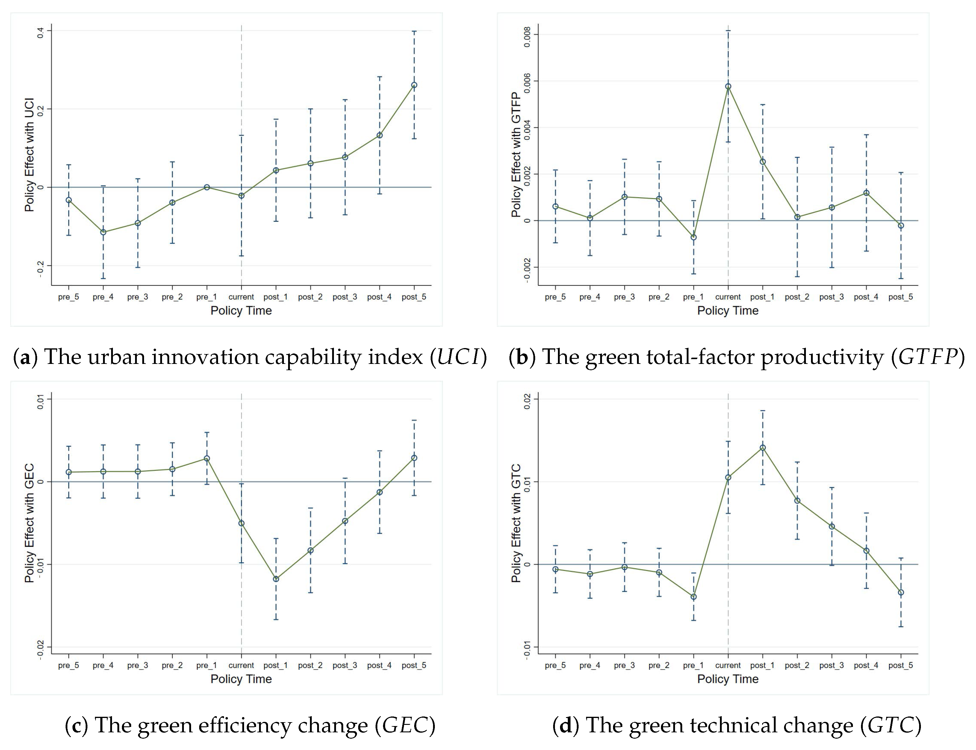
5.1. Parallel Trend Test

The classical differential method requires that the experimental group and the control group meet the parallel trend hypothesis before the implementation of the policy, that there is no significant difference before the implementation of the policy, and there is a significant difference after the implementation of the policy (that is, the regression coefficient before the implementation of the policy is not significant, but the regression coefficient is significant after the implementation of the policy) to verify whether the changing trend of the experimental group and the control group before and after the implementation of the policy is different. Therefore, for the relevant dependent variables of this paper, the urban innovation capability index ($UCI$) and green total-factor productivity ($GTFP$), a parallel trend test was conducted on the green efficiency change ($GEC$) and the green technical change ($GTC$). Figure 1a–d show the change in the regression coefficient before and after the implementation of smart pilot cities. The horizontal axis $post$ is posted after the policy is implemented, $pre$ is before the policy is implemented, and 0 is the base period.

It can be observed from Figure 1a–d that pilot cities had no significant impact on any of the dependent variables ($UCI$, $GTFP$, $GEC$, and $GTC$) before the construction of smart-city policies. Still, after the implementation of smart-city policies, different dependent variables showed various effects. On the one hand, Figure 1a, Figure 1b, and Figure 1d, respectively, show that, after a smart-city pilot policy, the urban innovation capacity index, green total-factor productivity, and green technology changes showed an inevitable upward trend, which is reflected as a positive impact. In addition, the $GTFP$ and $GTC$ had a positive impact on policy implementation in the current period, with a time lag effect of one to three periods, while the $UCI$ had no significant impact on policy implementation in the current period but a significant positive effect on the lag period of five periods. On the other hand, Figure 1c shows a negative impact after the implementation of the smart-city pilot policy, which means the green efficiency change had a specific downward trend. It can be seen that all the samples studied in this paper met the parallel trend test.

5.2. Regression Results and Discussion

5.2.1. Basic Regressions

In this study, the traditional DID model was used as the benchmark regression model. The results in

Table 3. Classic DID baseline regressions.

Variables	$UCI$		$GTFP$
Model	Model (1)	Model (2)	Model (3)	Model (4)
Effect	RE	FE	RE	FE
$DID$	0.4002 ***	0.4224 ***	0.0005	−0.0007
	(18.54)	(18.97)	(1.25)	(−1.28)
$edexp$	0.5107 ***	0.7000 ***	0.0008 **	0.0004
	(20.93)	(22.89)	(2.31)	(0.50)
$bua$	0.5444 ***	0.4627 ***	−0.0044 ***	−0.0053 ***
	(19.86)	(14.04)	(−11.96)	(−6.29)
$pgdp$	0.1028 ***	−0.0707 *	−0.0002	0.0003
	(3.63)	(−1.95)	(−0.61)	(0.34)
$eoye$	0.0052	−0.0203	0.0022 ***	0.0065 ***
	(0.22)	(−0.78)	(5.69)	(9.67)
$sciexp$	0.1435 ***	0.1173 ***	0	0.0003
	(9.92)	(7.75)	(−0.15)	(0.83)
$Constant$	−10.2962 ***	−9.9530 ***	0.9854 ***	0.9315 ***
	(−33.16)	(−29.33)	(195.91)	(107.16)
$Fixedeffect$	No	Yes	No	Yes
N	3892.00	3892.00	3892.00	3892.00
$R^2$	0.73	0.73	0.02	0.03
$Hausmantest$	chi2(6) = 101.80		chi2(6) = 69.85
	(p = 0.0000)		(p = 0.0000)
Variables	$GEC$		$GTC$
Model	Model (5)	Model (6)	Model (7)	Model (8)
Effect	RE	FE	RE	FE
$DID$	−0.0017	−0.0046 **	0.0026 **	0.0043 **
	(−1.35)	(−2.44)	(2.05)	(2.29)
$edexp$	−0.0003	−0.0016	0.0017 *	0.002
	(−0.25)	(−0.62)	(1.66)	(0.79)
$bua$	−0.0043 ***	−0.0027	−0.0001	−0.0021
	(−3.80)	(−0.96)	(−0.05)	(−0.77)
$pgdp$	−0.0003	0.0012	0.0005	−0.0001
	(−0.31)	(0.39)	(0.50)	(−0.05)
$eoye$	0.0012	0.0062 ***	0.0006	−0.0001
	(0.97)	(2.77)	(0.53)	(−0.06)
$sciexp$	0.0004	0.0008	−0.0005	−0.0002
	(0.58)	(0.60)	(−0.66)	(−0.17)
$Constant$	1.0172 ***	0.9445 ***	0.9612 ***	0.9804 ***
	(64.86)	(32.66)	(61.99)	(34.19)
$Fixedeffect$	No	Yes	No	Yes
N	3892.00	3892.00	3892.00	3892.00
$R^2$	0.00	0.00	0.00	0.00
$Hausmantest$	chi2(6) = 10.71		chi2(6) = 2.28
	(p = 0.0978)		(p = 0.8927)

Notes: * p < 0.10, ** p < 0.05, *** p < 0.01, and the t value is in parentheses. When the p-value of the regression coefficient is less than 0.1, 0.05, or 0.01, it indicates that the null hypothesis can be rejected at the 10%, 5%, or 1% significance level, thus supporting the alternative hypothesis. However, if the p-value of the regression coefficient is greater than 0.1, it indicates that the null hypothesis cannot be rejected at any of the commonly used significance levels, thereby confirming that the null hypothesis is true. The same as below.

show the regression results of the benchmark model, and the estimated results obtained using fixed effects and random effects are listed, respectively.

As shown in Table 3, through the Hausman test of fixed-effect and random-effect models, it was found that there were fixed effects in the regression models of the innovation index ($UCI$) and the green total-factor productivity ($GTFP$). However, in the regression results of the green efficiency change ($GEC$) and the green technical change ($GTC$), the fixed effect was not significant, so the random effect results could be selected for analysis. So, the policy-effect coefficient of the main explanatory variable innovation index ($UCI$) and the green technical change ($GTC$) were significantly positive, according to Model (2) and Models (7), indicating that the construction of smart pilot cities promotes the improvement of urban innovation capacity and the green technical change. However, the policy effect coefficient of the green total-factor productivity ($GTFP$) and the green efficiency change ($GEC$) did not significantly refer to Model (4) or Model (5), indicating that smart pilot-city construction has no significant effect on the sustainable development or the green efficiency change of a city. The above is only a preliminary conclusion, but the spatial effect of each variable was not taken into account. Therefore, the spatial effect of each variable needed to be added later for analysis.

5.2.2. Spatial Effect Regressions

The traditional DID model may have the problem of missing variables, resulting in unrobust regression results. The above analysis shows that, due to the connection between cities, urban innovation efficiency and sustainable development levels do not change independently. A city’s innovation efficiency and level of sustainable development may be influenced by the relevant policies or economic actions of other cities in the city network. Therefore, a DID-spatial Durbin model with spatial considerations is needed to more accurately estimate the impact of smart pilot-city policies on $UCI$ and sustainable development. The DID-spatial Durbin model can control the influence of missing variables and consider the spatial spillover effect. By incorporating the spatial adjacency matrix, the model can capture the spatial interconnections between cities, thus obtaining more robust regression results. Therefore, this study used the DID-spatial Durbin model to analyze the impact of smart pilot-city policies on $UCI$ and sustainable development. The premise of using the spatial metrology model is the existence of a spatial correlation among cities. In this study, Moran’s I index test was conducted using the anti-geographic distance matrix to test whether there was a spatial effect on urban innovation efficiency. The results are shown in

Table 4. Moran’s I test with $UCI,GTFP,GEC$, and $GTC$.

Variables	$\mathit{UCI}$	$\mathit{GTFP}$	$\mathit{GEC}$	$\mathit{GTC}$
2007	0.064 *	0.082 ***	0.125 ***	0.169 **
2008	0.097 **	0.167 ***	0.266 ***	0.245 ***
2009	0.142 ***	0.141 ***	0.237 ***	0.224 ***
2010	0.183 ***	0.159 ***	0.223 ***	0.220 ***
2011	0.221 ***	0.115 ***	0.113 ***	0.122 ***
2012	0.254 ***	0.079 **	0.144 ***	0.121 ***
2013	0.275 ***	0.088 **	0.391 ***	0.350 ***
2014	0.291 ***	−0.075 *	0.187 ***	0.376 ***
2015	0.312 ***	0.01	0.046	0.280 ***
2016	0.335 ***	0.058	0.015	0.066 *
2017	0.347 ***	0.118 ***	0.127 ***	0.183 ***
2018	0.363 ***	0.434 ***	0.281 ***	0.371 ***
2019	0.369 ***	0.218 ***	0.361 ***	0.378 ***
2020	0.380 ***	0.08 **	−0.019	0.169 ***

Notes: * p < 0.10, ** p < 0.05, *** p < 0.01, and the t value is in parentheses.

.

The Moran’s I index of the $UCI,GTFP,GEC$, and $GTC$ from 2007 to 2020 were almost significant and generally showed an increasing trend year by year, which basically could indicate that these variables all have a spatial correlation [75]. Therefore, the spatial econometric model could be used to study how the innovation capacity, green total-factor productivity, green efficiency change, and green technical change of cities may be affected by the relevant policies or economic behaviors of other cities in a city network.

To further investigate the impact of policy actions on urban innovation efficiency and sustainable development, this study incorporated a spatial-adjacency matrix in the DID-spatial Durbin model, and the regression results are shown in

Table 5. Results of SDM regression with spatial-adjacency matrix.

Variables	$UCI$		$GTEP$
Model	Model (9)	Model (10)	Model (11)	Model (12)
$DID$	0.3609 ***	0.2796 ***	−0.0006	−2.0012 **
	(21.46)	(16.78)	(−2.47)	(−2.22)
$edexp$		0.2381 ***		0.0002
		(10.80)		(0.40)
$bua$		0.3312 ***		−2.0069 ***
		(13.84)		(−20.73)
$pgdp$		−2.1388 ***		0.0048 ***
		(−2.62)		(7.08)
$eoye$		0.0621 ***		0.0083 ***
		(3.35)		(14.46)
$sciexp$		0.0800 ***		−2.0007 **
		(7.35)		(−2.07)
$Constant$	0.1846 ***	−2.1885 ***	0.9980 ***	0.8368 ***
	(3.30)	(−24.73)	(741.45)	(93.34)
$W_n\ast DID$	0.1163 ***	−2.1008 ***	0.0009	−2.0029 ***
	(4.30)	(−2.56)	(1.42)	(−2.33)
$\rho$	0.7690 ***	0.6194 ***	0.0037 ***	0.0450 ***
	(84.97)	(51.10)	(2.70)	(13.04)
${\sigma }_e^2$	0.0802 ***	0.0759 ***	0.0001 ***	0.0001 ***
	(40.99)	(40.65)	(42.48)	(41.85)
N	3892	3892	3892	3892
$R^2$	0.238	0.667	0.002	0.005
$DID$	−2.0048 ***	−2.0049 ***	0.0053 ***	0.0050 ***
	(−2.31)	(−2.28)	(5.35)	(4.84)
Variables	$GEC$		$GTC$
Model	Model (13)	Model (14)	Model (15)	Model (16)
$edexp$		−2.0003		−2.0011
		(−2.18)		(−2.82)
$bua$		−2.0036 **		0.0006
		(−2.20)		(0.41)
$pgdp$		−2.0016		0.0048 ***
		(−2.91)		(2.99)
$eoye$		0.0045 ***		−2.0006
		(3.43)		(−2.48)
$sciexp$		0.0009		−2.0009
		(1.19)		(−2.40)
$Constant$	0.2826 ***	0.2529 ***	0.2362 ***	0.2136 ***
	(24.50)	(11.69)	(22.37)	(10.93)
$W_n\ast DID$	0.0048 ***	0.0056 ***	−2.0050 ***	−2.0069 ***
	(3.23)	(3.00)	(−2.81)	(−2.13)
$\rho$	0.7361 ***	0.7369 ***	0.7786 ***	0.7795 ***
	(76.40)	(76.69)	(92.72)	(92.94)
${\sigma }_e^2$	0.0004 ***	0.0004 ***	0.0003 ***	0.0003 ***
	(40.21)	(40.20)	(40.34)	(40.33)
N	3892	3892	3892	3892
$R^2$	0.0000	0.0000	0.0000	0.0000

Notes: ** p < 0.05, *** p < 0.01, and the t value is in parentheses.

. Overall, the regression results of the SDM model are consistent with those of the traditional DID regression, indicating that the SDM model is more robust.

Based on the SDM regression results in Table 5, it was found that the impact of the smart pilot-city policy on $UCI$ and $GTFP$ was mainly reflected in two aspects. Firstly, the policy had a direct positive effect on innovation capacity, which was verified according to the significant positive coefficient of the policy dummy variable DID in Model (10), indicating that the smart pilot-city policy had a facilitating effect on the improvement of innovation capacity. This also verifies the reasonableness of H1_1. Policies have a direct negative impact on $GTFP$, which was verified according to the significant negative coefficient of the policy dummy variable DID. This indicates that smart pilot-city policies may inhibit the sustainable development of cities. This is inconsistent with the non-significant conclusion obtained using the panel regression Model (4) in Table 3, so the situation of H2_0 may occur. Secondly, there was a spillover effect of smart pilot-city policy on $UCI$, $GTFP$, $GEC$, and $GTC$. The coefficients of the spatial lag term ($W_n\ast DID$) of the policy dummy variables in models (10), (12), (14), and (16) were significantly negative or positive at the 5% level, and the coefficients that inhibit the spillover effect on $UCI$, $GTFP$, and $GTC$ while having a positive spillover effect on $GEC$ were all significantly negative or positive. This indicates that the construction of smart cities can effectively promote the $GEC$ of neighboring cities, the policy of smart pilot cities has an “inhibitory” effect on the $UCI$, $GTFP$, and $GTC$ of neighboring cities, and the policy of smart pilot cities can promote the sustainable development of neighboring cities. This verifies H3a_1.

The reason for this is that the construction of smart cities is often concentrated in one city, leading to a high concentration of resources and technologies. This concentration may put neighboring cities at a disadvantage in terms of access to resources and technological support, thereby limiting their innovative activities. For example, smart cities may attract large amounts of talent, capital, and technology, making it difficult for neighboring cities to access these resources in order to drive innovation. The development of smart cities may trigger a “catch-up effect” in neighboring cities, whereby neighboring cities have to invest more in similar developments to remain competitive. However, such catching up may not be based on their own development needs and realities but, rather, on blind imitation, leading to a waste of resources and inefficiency [77]. At the same time, neighboring cities may face technical, financial, and managerial challenges in the process of catching up, further inhibiting their $UCI$, $GTFP$, and $GTC$. The construction of smart cities may intensify the competition between cities, leading to less cooperation between neighboring cities. This competitive relationship may result in a lack of cooperation mechanisms such as information sharing and technology exchange between cities, thus limiting the scope and depth of innovation activities. This makes the negative spatial spillover effect of the smart pilot-city policy on $UCI$, $GTFP$, and $GTC$ more prominent. This also validates H3a_1 of the study.

5.3. Robustness Test

5.3.1. Variable Substitution

To check whether the SDM regression model is robust to various potential interfering factors, this study tried different combinations of control variables to observe whether the coefficients and significance levels of the core explanatory variables changed significantly, as shown in

Table 6. Results of variable substitution regression.

Variables	$UCI$		$GTEP$
Model	Model (9)	Model (10)	Model (11)	Model (12)
$DID$	0.3609 ***	0.2725 ***	−2.0006	−2.0002
	(21.46)	(16.68)	(−2.47)	(−2.46)
$fina$		−2.1921 ***		0.0032 ***
		(−2.39)		(4.56)
$bua$		0.3109 ***		−2.0019 ***
		(13.57)		(−2.30)
$gdp$		0.4727 ***		−2.0027 ***
		(13.30)		(−2.22)
$sis$		−2.7221 ***		0.0103 ***
		(−28.01)		(9.23)
$sciexp$		0.0953 ***		0.0010 ***
		(8.50)		(2.95)
$Constant$	0.1846 ***	0.4368	0.9980 ***	0.9031 ***
	(3.30)	(1.50)	(741.45)	(100.95)
$W_n\ast DID$	0.1163 ***	−2.1385 ***	0.0009	−2.0006
	(4.30)	(−2.96)	(1.42)	(−2.74)
$\rho$	0.7690 ***	0.5489 ***	0.0037 ***	0.0305 ***
	(84.97)	(42.12)	(2.70)	(12.39)
${\sigma }_e^2$	0.0802 ***	0.0740 ***	0.0001 ***	0.0001 ***
	−20.99	−20.92	−22.48	−22.13
N	3892	3892	3892	3892
$R^2$	0.238	0.727	0.002	0.009
Variables	$GEC$		$GTC$
Model	Model (13)	Model (14)	Model (15)	Model (16)
$DID$	−2.0048 ***	−2.0040 ***	0.0053 ***	0.0047 ***
	(−2.31)	(−2.53)	(5.35)	(4.55)
$fina$		0.0039 **		−2.0021
		(2.01)		(−2.18)
$bua$		−2.0019		0.0004
		(−2.16)		(0.30)
$gdp$		−2.0074 ***		0.0041 *
		(−2.80)		(1.72)
$sis$		0.0109 ***		−2.0095 ***
		(4.02)		(−2.90)
$sciexp$		0.0012		−2.0003
		(1.53)		(−2.45)
$Constant$	0.2826 ***	0.2350 ***	0.2362 ***	0.2776 ***
	(24.50)	(10.28)	(22.37)	(12.90)
$W_n\ast DID$	0.0048 ***	0.0077 ***	−2.0050 ***	−2.0077 ***
	(3.23)	(4.06)	(−2.81)	(−2.50)
$\rho$	0.7361 ***	0.7333 ***	0.7786 ***	0.7764 ***
	(76.40)	(75.67)	(92.72)	(91.94)
${\sigma }_e^2$	0.0004 ***	0.0004 ***	0.0003 ***	0.0003 ***
	(40.21)	(40.22)	(40.34)	(40.33)
N	3892	3892	3892	3892
$R^2$	0.0000	0.0000	0.0000	0.0000

Notes: * p < 0.10, ** p < 0.05, *** p < 0.01, and the t value is in parentheses.

.

The innovation capacity of smart pilot cities is influenced not only by the per-capita GDP of education expenditure but also by the financial expenditure, the proportion of the GDP of the whole city, and the GDP of secondary industries. Therefore, this study further analyzed the impact of smart pilot cities on $UCI$, $GTFP$, $GEC$, and $GTC$ in the case of urban network externalities by rebuilding the spatial weight matrix based on the adjacency matrix of variables. In the stable bond regression results for $GTFP$, it was found that the impact of smart-city construction on urban $GTFP$ is still not significant, which is consistent with the conclusion of Model (4) in Table 3 but inconsistent with the conclusion of Model (12) in Table 5, indicating that the impact of smart-city construction on the sustainable development of a city is not stable. In Table 5 of spatial regression results and Table 6 of steady-key regression results, the regression results of other variables are consistent except for differences in the impact of smart-city policies on $GTFP$. At the same time, it was found that the influence of smart-city policy construction on $GEC$ and $GTC$ were in opposite directions, which was precisely because of the effects of these two variables; the impact of a smart city on urban green total-factor productivity may not be significant. At the same time, the theoretical H1_1, H2_0, and H3a_1 proposed above were verified again.

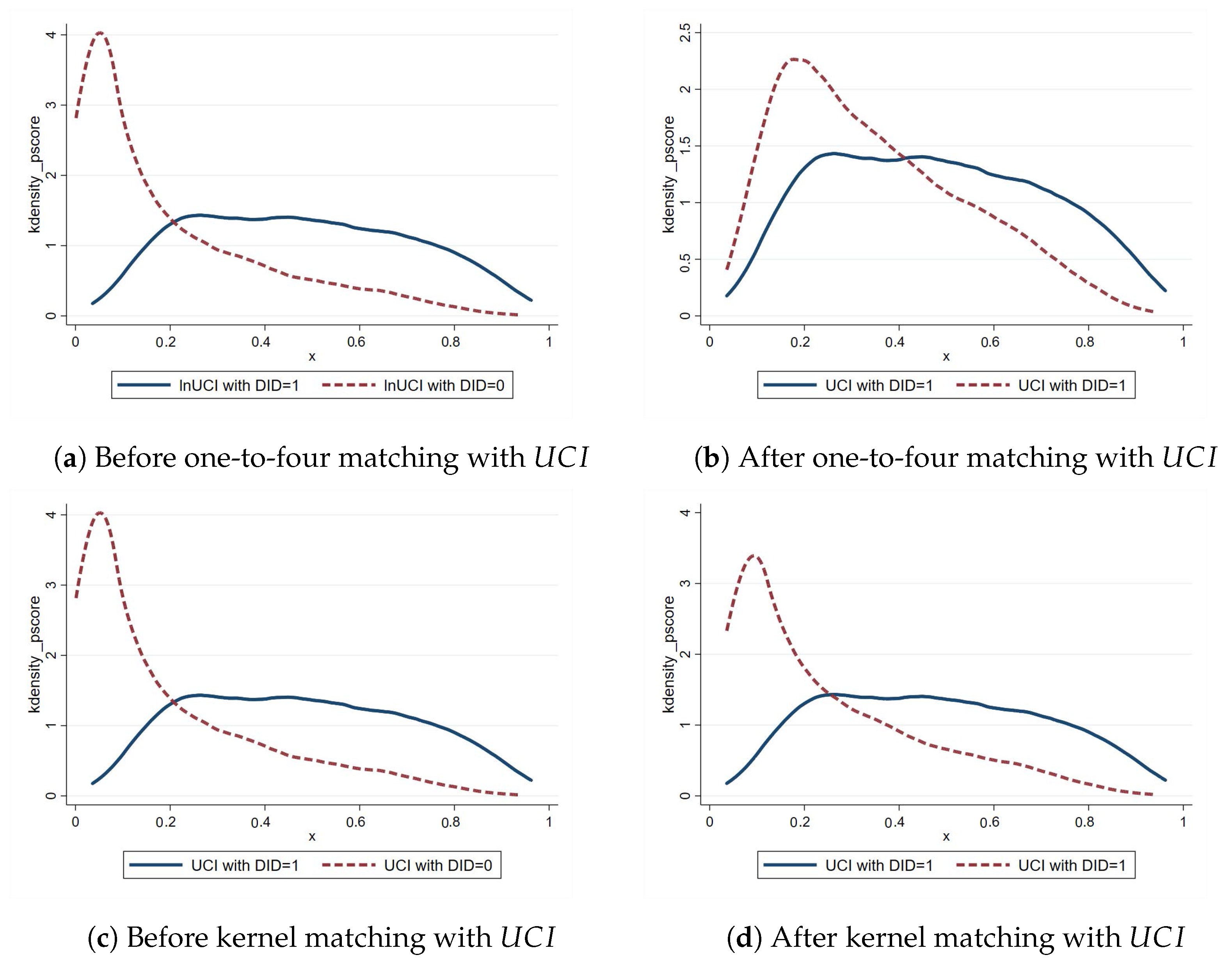
5.3.2. Propensity Score-Matching Method and Difference-in-Difference (PSM-DID)

The above analysis results show the following: (1) The construction of smart cities can enhance the innovation efficiency of a city. (2) The construction of smart cities has a spatial effect and can influence the $UCI$ and $GTFP$ of surrounding cities through urban network externalities. (3) The construction of smart cities may inhibit or have no significant effect on the $GTFP$ of a city. However, the selection of which cities are to implement smart-city pilots is not random, and there may be a high level of $UCI$ or a low level of $GTFP$ in these cities, so the data may be biased. To further discuss the stability of the above conclusions, this section presents a regression test that was conducted on the impact of smart-city construction on $UCI$ and $GTFP$ based on PSM-DID. The propensity-matching score was mainly selected from one to four matching and kernel-matching methods, and the distribution diagram of the matched data was tested. The variable $UCI$ was taken as an example to show its progress, as depicted in Figure 2.

It can be found from the results of Figure 2, by comparing the probability density distribution maps before and after data matching, that the matching effect of one-to-four was revealed to be better than that of kernel-density matching, and both of them had a certain effect on the similarity of the data distribution. Based on the above matching data of one-to-four matching and nuclear matching, and combined with Formula (3), the effect of smart-city policy construction was analyzed, and the results are shown in

Table 7. PSM-DID regression results.

Variable	$UCI$
Matching	One-to-four matching			Kernel matching
$DID$	1.2529 ***	0.6907 ***	0.4016 ***	30.0451 ***	23.2986 ***	22.1134 ***
	(29.46)	(14.98)	(15.45)	(19.93)	(13.00)	(12.97)
$W_n\ast DID$		0.2982 ***	−2.0075		3.3642 ***	0.1006
		(21.74)	(−2.84)		(6.84)	(0.20)
$W_n\ast UCI$			0.1772 ***			0.0932 ***
			(66.27)			(17.83)
$Constant$	1.2891 ***	0.9434 ***	0.1413 ***	4.1034 ***	0.9566	−2.0712
	(59.64)	(37.59)	(7.65)	(5.89)	(1.15)	(−2.09)
N	2241	2241	2241	3246	3246	3246
$R^2$	0.307	0.441	0.827	0.118	0.132	0.216
Variable	$GTFP$
Matching	One-to-four matching			Kernel matching
$DID$	−2.0007	0.0009	0.0008	−2.0006	0.0001	−2.0001
	(−2.75)	(0.73)	(0.72)	(−2.09)	(0.09)	(−2.11)
$W_n\ast DID$		−2.0009 **	−2.0006 *		−2.0003 *	−2.0001
		(−2.41)	(−2.87)		(−2.81)	(−2.59)
$W_n\ast GTFP$			0.1329 ***			0.1253 ***
			(18.60)			(22.14)
$Constant$	1.0022 ***	1.0032 ***	0.3534 ***	1.0021 ***	1.0024 ***	0.3907 ***
	(1979.69)	(1534.55)	(10.12)	(3799.15)	(3164.20)	(14.14)
N	2241	2241	2241	3246	3246	3246
$R^2$	0	0.003	0.153	0	0.002	0.143
Variable	$GEC$
Matching	One-to-four matching			Kernel matching
$DID$	−2.0089 ***	−2.0092 **	−2.0077 ***	−2.0066 ***	−2.0059 ***	−2.0061 ***
	(−2.76)	(−2.35)	(−2.64)	(−2.48)	(−2.60)	(−2.69)
$W_n\ast DID$		0.0001	0.0001		−2.0003	0.0007 *
		(0.11)	(0.17)		(−2.55)	(1.96)
$W_n\ast GEC$			0.1723 ***			0.1728 ***
			(68.57)			(77.14)
$Constant$	1.0131 ***	1.0130 ***	0.1638 ***	1.0125 ***	1.0129 ***	0.1614 ***
	(615.67)	(475.99)	(13.17)	(1157.79)	(963.80)	(14.60)
N	2241	2241	2241	3246	3246	3246
$R^2$	0.004	0.004	0.707	0.004	0.004	0.669
Variable	$GTC$
Matching	One-to-four matching			Kernel matching
$DID$	0.0094 ***	0.0108 ***	0.0089 ***	0.0072 ***	0.0067 ***	0.0065 ***
	(2.92)	(2.76)	(4.60)	(3.84)	(2.96)	(5.41)
$W_n\ast DID$		−2.0007	−2.0007		0.0003	−2.0008 **
		(−2.62)	(−2.23)		(0.45)	(−2.41)
$W_n\ast GTC$			0.1742 ***			0.1752 ***
			(77.09)			(87.19)
$Constant$	0.9899 ***	0.9908 ***	0.1474 ***	0.9903 ***	0.9901 ***	0.1451 ***
	(604.16)	(467.60)	(13.41)	(1139.90)	(948.35)	(14.94)
N	2241	2241	2241	3246	3246	3246
$R^2$	0.004	0.005	0.753	0.005	0.005	0.721

Notes: * p < 0.10, ** p < 0.05, *** p < 0.01, and the t value is in parentheses.

.

The following can be seen from the results in Table 7: (1) At the 1% level, smart-city construction had a significant positive impact on urban innovation ($UCI$), and urban innovation had a significant positive spatial spillover effect, while the policy space had a certain positive spatial spillover effect, but the effect was unstable, regardless of whether the spatial effect variables of policy and the urban innovation index were added. (2) Regardless of one-to-four matching or nuclear matching, in the regression results obtained, smart-city construction policies had no significant impact on the green total-factor productivity of cities. However, at the 10% level, smart-city construction had a significant negative spatial effect on the green total-factor productivity of neighboring cities. Moreover, urban green total-factor productivity ($GTFP$) had a significant positive spatial effect on the development of urban green total-factor productivity in neighboring cities. (3) At the 5% level, smart-city construction had a significant negative impact on urban green efficiency change ($GEC$). In addition, there were positive spatial spillover effects and positive policy spatial effects for the green efficiency change. (4) At the 5% level, smart-city construction had a significant positive impact on the green technical change ($GTC$), and there was a significant positive spatial spillover effect and negative policy spatial effect of the green technical change, but similarly. Thus, H1_1, H2_0, and H3a_1 were tested again.

6. Further Results and Discussion

6.1. Regional Difference Analysis

The impact of smart pilot-city policies on innovation and sustainable development is different in different regions. In this section of the study, the experimental data were divided into three regions, eastern, central, and western, according to China’s regional divisions to analyze the differences in city regions and gain a more intuitive understanding of the impact of the smart pilot-city policy on different regions. The results are shown in

Table 8. Results of SDM regression with spatial-adjacency matrix in three regions.

Variables	Eastern
	$UCI$	$GTFP$	$GEC$	$GTC$
Model	Model (25)	Model (26)	Model (27)	Model (28)
$DID$	0.3442 ***	−2.0006	−2.0086 ***	0.0062 ***
	(11.20)	(−2.57)	(−2.64)	(2.90)
$W_n\ast DID$	−2.1123 **	0.0029 **	0.0016	−2.0037
	(−2.19)	(2.12)	(0.45)	(−2.16)
$\rho$	0.5539 ***	0.0003	0.6916 ***	0.7539 ***
	(25.26)	(0.15)	(39.84)	(51.52)
$Controls$	Yes	Yes	Yes	Yes
N	1344	1344	1344	1344
$Citiesnum$	96	96	96	96
$R^2$	0.745	0.078	0.000	0.001
Variables	Central
	$UCI$	$GTFP$	$GEC$	$GTC$
Model	Model (29)	Model (30)	Model (31)	Model (32)
$DID$	0.1954 ***	0.0000	−2.0006	0.0005
	(7.72)	(0.04)	(−2.52)	(0.55)
$W_n\ast DID$	−2.0034	0.0013	0.0055 ***	−2.0036 **
	(−2.08)	(1.36)	(2.80)	(−2.15)
$\rho$	0.6265 ***	0.3866 ***	0.7777 ***	0.8073 ***
	(29.48)	(13.18)	(57.96)	(68.36)
$Controls$	Yes	Yes	Yes	Yes
N	1400	1400	1400	1400
$Citiesnum$	100	100	100	100
$R^2$	0.662	0.07	0.007	0.008
Variables	Western
	$UCI$	$GTFP$	$GEC$	$GTC$
Model	Model (33)	Model (34)	Model (35)	Model (36)
$DID$	0.3828 ***	0.0011 **	−2.0062 ***	0.0075 ***
	(12.02)	(2.07)	(−2.91)	(3.89)
$W_n\ast DID$	−2.0775	0.0001	0.0073 **	−2.0094 ***
	(−2.55)	(0.14)	(2.33)	(−2.32)
$\rho$	0.3383 ***	0.0016	0.6326 ***	0.6698 ***
	(12.18)	(1.57)	(32.45)	(38.04)
$Controls$	Yes	Yes	Yes	Yes
N	1148	1148	1148	1148
$Citiesnum$	82	82	82	82
$R^2$	0.614	0.048	0.000	0.000

Notes: ** p < 0.05, *** p < 0.01, and the t value is in parentheses.

.

From the results of Table 8, it can be seen from models (25), (29), and (33) that the policy has a positive and significant impact and a positive spatial spillover effect on the innovation level of eastern, central, and western China; the average direct effect was 0.3442, 0.1954, and 0.3828, respectively. The average spatial spillover effects were 0.5539, 0.6265, and 0.3383, respectively. This indicates that the direct promotion effect of smart-city construction in the central region was the lowest, while the spatial spillover effect was the highest, and the direct promotion effect of smart-city construction in the western region was the highest, while the spatial spillover effect was the lowest. In addition, the spatial spillover effect of smart-city policy effects was significantly negative only in the eastern region but not in the central and western areas.

At the same time, it can be seen from models (26), (30), and (34) that the impact of smart-city construction on urban green total-factor productivity ($GTFP$) was different in different regions. The western region had a significant positive effect, but the eastern and central regions had no significant impact. Only the central region had a significant positive spatial spillover effect on green total-factor productivity, and the eastern region had a considerable polity-positive spatial spillover effect on green total-factor productivity.

In addition, the results of the remaining regression results revealed that the eastern and western regions had a significant effect on the change in the green effect and green technology change, in which the former was significantly negative, the latter was significantly positive, and there was a significant policy spatial effect in the central and western regions. In other words, the implementation of policies in cities of the western and central areas would promote the green effect or inhibit the green technology of cities in the neighboring regions, respectively. On the whole, there were significant positive spatial spillover effects for the urban green effect and green technology in the eastern, central, and western regions. This tested H3b_1.

To further analyze the impact of policy effects on $UCI$ and $GTFP$ in different regions, the region was further divided into seven regions: northeast, north, central, south, east, northwest, and southwest, and the regression results are shown in

Table 9. Results of SDM regression with spatial-adjacency matrix in seven regions.

Variables	Northeast
	$UCI$	$GTFP$	$GEC$	$GTC$
Model	Model (37)	Model (38)	Model (39)	Model (40)
$DID$	0.2346 ***	−2.0015	−2.001	0.0006
	(4.87)	(−2.77)	(−2.26)	(0.21)
$W_n\ast DID$	0.014	−2.0106 ***	0.0005	−2.0049
	(0.18)	(−2.29)	(0.10)	(−2.02)
$\rho$	0.4765 ***	0.0149 ***	0.6522 ***	0.7610 ***
	(11.20)	(3.87)	(19.17)	(30.49)
$Controls$	Yes	Yes	Yes	Yes
N	504	504	504	504
$Citiesnum$	36	36	36	36
$R^2$	0.737	0.02	0.001	0.002
Variables	North
	$UCI$	$GTFP$	$GEC$	$GTC$
Model	Model (41)	Model (42)	Model (43)	Model (44)
$DID$	0.4262 ***	−2.0039 ***	−2.0084 *	0.0075 *
	(12.64)	(−2.89)	(−2.92)	(1.86)
$W_n\ast DID$	−2.2565 ***	−2.0035 *	0.006	−2.0089
	(−2.38)	(−2.70)	(0.88)	(−2.41)
$\rho$	0.5133 ***	0.0136 **	0.6555 ***	0.7120 ***
	(13.41)	(2.52)	(20.67)	(25.73)
$Controls$	Yes	Yes	Yes	Yes
N	420	420	420	420
$Citiesnum$	30	30	30	30
$R^2$	0.519	0.015	0	0
Variables	Midland
	$UCI$	$GTFP$	$GEC$	$GTC$
Model	Model (45)	Model (46)	Model (47)	Model (48)
$DID$	0.2181 ***	0.0001	−2.0018	0.0019
	(5.70)	(0.12)	(−2.95)	(1.10)
$W_n\ast DID$	0.1247 *	0.0032 **	0.0072 *	−2.0034
	(1.68)	(2.20)	(1.94)	(−2.01)
$\rho$	0.5661 ***	0.4289 ***	0.7788 ***	0.7906 ***
	(15.95)	(9.96)	(40.73)	(43.68)
$Controls$	Yes	Yes	Yes	Yes
N	588	588	588	588
$Citiesnum$	42	42	42	42
$R^2$	0.69	0.121	0.009	0.01
Variables	South
	$UCI$	$GTFP$	$GEC$	$GTC$
Model	Model (49)	Model (50)	Model (51)	Model (52)
$DID$	0.3743 ***	0.0011	−2.0009	0.0018
	(6.73)	(0.60)	(−2.38)	(0.90)
$W_n\ast DID$	−2.1117	0.0064 **	0.0114 ***	−2.005
	(−2.15)	(2.12)	(2.95)	(−2.43)
$\rho$	0.6163 ***	0.0804	0.6994 ***	0.7462 ***
	(17.71)	(1.39)	(25.36)	(29.72)
$Controls$	Yes	Yes	Yes	Yes
N	490	490	490	490
$Citiesnum$	35	35	35	35
$R^2$	0.807	0.087	0.035	0.015
Variables	Eastland
	$UCI$	$GTFP$	$GEC$	$GTC$
Model	Model (53)	Model (54)	Model (55)	Model (56)
$DID$	0.1778 ***	−2.0012	−2.0056 **	0.0051 ***
	(5.89)	(−2.04)	(−2.47)	(2.60)
$W_n\ast DID$	−2.2040 ***	0.0001	0.0048	−2.0047
	(−2.21)	(0.07)	(1.38)	(−2.55)
$\rho$	0.6952 ***	0.1164 ***	0.7740 ***	0.8202 ***
	(34.42)	(8.52)	(46.43)	(58.20)
$Controls$	Yes	Yes	Yes	Yes
N	1064	1064	1064	1064
$Citiesnum$	76	76	76	76
$R^2$	0.682	0.008	0	0
Variables	Northwest
	$UCI$	$GTFP$	$GEC$	$GTC$
Model	Model (57)	Model (58)	Model (59)	Model (60)
$DID$	0.2975 ***	0.0015 *	−2.0037	0.0051 *
	(6.36)	(1.91)	(−2.15)	(1.83)
$W_n\ast DID$	−2.1569 *	0.0012	0.0088 *	−2.0116 **
	(−2.91)	(0.92)	(1.68)	(−2.52)
$\rho$	0.1984 ***	0.0011	0.6419 ***	0.7097 ***
	(3.52)	(0.79)	(17.64)	(22.67)
Controls	Yes	Yes	Yes	Yes
N	420	420	420	420
$Citiesnum$	30	30	30	30
$R^2$	0.653	0.094	0.001	0
Variables	Southwest
	$UCI$	$GTFP$	$GEC$	$GTC$
Model	Model (61)	Model (62)	Model (63)	Model (64)
$DID$	0.2581 ***	0.0013	−2.002	0.0031
	(4.14)	(1.18)	(−2.78)	(1.36)
$W_n\ast DID$	0.1692 *	0.0026	0.0067 *	−2.0046
	(1.76)	(1.63)	(1.74)	(−2.37)
$\rho$	0.2481 ***	0.2723 ***	0.6715 ***	0.6893 ***
	(5.56)	(5.71)	(24.65)	(26.67)
Controls	Yes	Yes	Yes	Yes
N	406	406	406	406
$Citiesnum$	29	29	29	29
$R^2$	0.722	0.052	0.011	0.004

Notes: * p < 0.10, ** p < 0.05, *** p < 0.01, and the t value is in parentheses.

.

According to models (37), (41), (45) (49), (53), (57), and (61), in Table 9, the regression results show that, among the regression results of $UCI$, there were significant positive direct policy effects and indirect spatial spillover effects in different regions, among which the direct policy effects were 0.2346, 0.4262, 0.2181, 0.3743, 0.1778, 0.2975, and 0.2581, respectively. The direct policy average effect in the midland region was the largest, followed by that in the south region. The east region had the smallest indirect spatial spillover effect, and the indirect spatial spillover effect was 0.4765, 0.5133, 0.5661, 0.6163, 0.6952, 0.198, and 0.2481, respectively. The east region had the most significant indirect spatial spillover effect, followed by the south region and northwest region. However, the spatial impacts of policies in the different areas were different, among which, the north, east, and northwest were significantly negative, the midland and southwest were significantly positive, and the northeast and south were not significant.

Similarly, from models (38), (42), (46) (50), (54), (58), and (62) in Table 9, it can be found that smart-city policies had no significant impact on urban green total-factor productivity in most regions. Only the northwest region had a significant positive effect at the 10% level. As for the regression results of the indirect spatial spillover effect and policy-spatial effect, it can be found that spatial effects were different in different regions. $GTFP$ had positive spatial spillover effects in the northeast, north, midland, east, and southwest regions. There was a negative spillover effect of the policy space in the northeast and north regions and a positive spillover effect in the midland and south regions.

From the remaining regression results in Table 9, it can be seen that the implementation of smart-city policies had a different significance on urban $GEC$ and $GTC$; some regions were significant, while others were not, but the symbols of influence on $GEC$ and $GTC$ were the opposite. At the same time, both $GEC$ and $GTC$ had significant positive spatial spillover effects on neighboring cities, while there were few areas with significant spillover effects of policies. This also verified H3b_1.

6.2. City Difference Analysis

The previous analysis from the perspective of different geographical regions in China indicates that there are regional differences in the impact of smart-city construction on urban innovation capability ($UCI$), green total-factor productivity ($GTEP$), green efficiency ($GEC$), and green technology progress ($GTC$). In addition to the regional disparities, the development status of different cities could also have affected the outcomes of this study. Therefore, this paper further categorized the development levels of cities based on the annual regional GDP quartiles: the lower quartile ($Q25$), the median ($Q50$), and the upper quartile ($Q75$). The categorization rules were as follows: if a city’s annual GDP was greater than or equal to the regional annual GDP’s upper quartile ($Q75$), the city was defined as a first-tier city for that year. If a city’s annual GDP was greater than or equal to the regional annual GDP median ($Q50$) but less than the regional annual GDP’s upper quartile ($Q75$), the city was defined as a second-tier city for that year. If a city’s annual GDP was greater than or equal to the regional annual GDP’s lower quartile ($Q25$) but less than the regional annual GDP median ($Q50$), the city was defined as a third-tier city for that year. If a city’s annual GDP was less than the regional annual GDP’s lower quartile ($Q25$), the city was defined as a fourth-tier city for that year. The regression results based on samples divided into different urban regions are shown in

Table 10. Results of SDM regression with spatial-adjacency matrix in four different city regions.

City	First-tier cities
Variables	$UCI$	$GTFP$	$GEC$	$GTC$
Model	Model (65)	Model (66)	Model (67)	Model (68)
$DID$	0.2982 ***	−2.002	−2.0110 ***	0.0096 ***
	(8.92)	(−2.19)	(−2.66)	(3.55)
$W_n\ast DID$	0.0372 ***	−2.0011 **	−2.0002	−2.0011
	(3.44)	(−2.03)	(−2.25)	(−2.21)
$\rho$	0.0013 ***	0.1455 ***	0.1907 ***	0.1947 ***
	(17.23)	(11.37)	(39.49)	(46.46)
$Controls$	Yes	Yes	Yes	Yes
N	966	966	966	966
$Citiesnum$	69	69	69	69
$R^2$	0.929	0.239	0.65	0.723
City	Second-tier cities
Variables	$UCI$	$GTFP$	$GEC$	$GTC$
Model	Model (69)	Model (70)	Model (71)	Model (72)
$DID$	0.3456 ***	−2.001	−2.0079 ***	0.0069 ***
	(9.39)	(−2.96)	(−2.21)	(3.09)
$W_n\ast DID$	0.0251 **	−2.0005 *	0.0005	−2.001
	(2.28)	(−2.66)	(0.71)	(−2.53)
$\rho$	0.0027 ***	0.1046 ***	0.1718 ***	0.1751 ***
	(19.56)	(12.18)	(48.15)	(53.27)
$Controls$	Yes	Yes	Yes	Yes
N	980	980	980	980
$Citiesnum$	70	70	70	70
$R^2$	0.848	0.209	0.731	0.769
	$UCI$	$GTFP$	$GEC$	$GTC$
City	Third-tier cities
Model	Model (73)	Model (74)	Model (75)	Model (76)
$DID$	0.1838 ***	0.0008	0.0009	0.0006
	(4.85)	(0.85)	(0.37)	(0.28)
$W_n\ast DID$	0.0629 ***	−2.0005 *	0.001	−2.0016 ***
	(5.76)	(−2.71)	(1.55)	(−2.65)
$\rho$	0.0019 ***	0.0846 ***	0.1556 ***	0.1552 ***
	(13.03)	(9.11)	(40.91)	(45.63)
$Controls$	Yes	Yes	Yes	Yes
N	980	980	980	980
$Citiesnum$	70	70	70	70
$R^2$	0.761	0.163	0.666	0.711
City	Fourth-tier cities
Variables	$UCI$	$GTFP$	$GEC$	$GTC$
Model	Model (77)	Model (78)	Model (79)	Model (80)
$DID$	0.1607 ***	−2.0005	−2.0007	0.0007
	(6.33)	(−2.82)	(−2.33)	(0.35)
$W_n\ast DID$	0.0431 ***	0.0002	0.0024 ***	−2.0022 ***
	(5.36)	(0.81)	(3.73)	(−2.66)
$\rho$	0.0032 ***	0.0697 ***	0.1593 ***	0.1582 ***
	(17.17)	(10.28)	(35.66)	(39.32)
$Controls$	Yes	Yes	Yes	Yes
N	966	966	966	966
$Citiesnum$	69	69	69	69
$R^2$	0.724	0.152	0.607	0.649

Notes: * p < 0.10, ** p < 0.05, *** p < 0.01, and the t value is in parentheses.

.

According to the regression results of $UCI$, in models (65), (69), (73), and (77) in Table 10, it can be seen that smart-city policies had significant positive direct and indirect impacts on the innovation capability of different cities. The average direct impact effect was 0.2982, 0.3456, 0.1838, and 0.1607, respectively. First-tier and second-tier cities had a more significant impact, while third-tier and fourth-tier cities had a more minor impact. This shows that the construction of smart cities has a more noticeable effect on the innovation capacity of cities with sound economic development. At the same time, the spatial indirect impact of policies was 0.0372, 0.0251, 0.0629, and 0.0431, respectively. Among them, the influence of first-tier and second-tier cities was relatively small. In contrast, the impact of third-tier and fourth-tier cities was more significant, which was the opposite of the direct-effect size distribution. This indicates that the smart-city construction policy of a city with weak economic development has a more obvious promoting effect on the innovation capacity of neighboring cities.

According to the regression results of $GTFP$, in models (66), (70), (74), and (78) in Table 10, smart-city policies had no significant impact on urban green total-factor productivity. Meanwhile, the spatial effect of urban green total-factor productivity was significantly positive. However, in first-tier, second-tier, and third-tier cities, smart-city policies had a significant negative spatial effect on urban green total-factor productivity at the 10% level.

According to the regression results of $GEC$ and $GTC$ in models (67), (68), (71), (72), (75), (76), (79), and (80) in Table 10, it can be seen that the impact of smart-city policies on urban green efficiency or urban technological progress was significantly negative or positive in first-tier and second-tier cities, respectively. However, it was not significant in third-tier and fourth-tier cities. That is, there were also regional differences in economic development. At the same time, the spatial effect of urban green efficiency or urban technological progress was significantly positive. However, in fourth-tier cities, smart-city policies had significant positive or negative policy-space spillover effects on urban green efficiency or urban technological progress at the 1% level, respectively. In contrast, in third-tier cities, smart-city policies only had significant adverse policy-space spillover effects on urban technological progress.

According to the value of regression coefficient $\rho$ in Table 10, at the 1% level, urban innovation capability ($UCI$), urban green productivity ($GTEP$), urban green efficiency ($GEC$), and green technology progress ($GTC$) all had significant positive spatial spillover effects in the four metropolitan regions. Most of them showed the following rule: the better the urban regional economic development, the greater the average spillover effect. This also tested H3b_1.

7. Conclusions, Policy Recommendations, and Further Research

7.1. Main Conclusions

Urban innovation capacity and urban green total-factor productivity are the keys to sustainable urban development. To study the impact of smart-city policies on urban innovation capacity and green total-factor productivity, this paper has analyzed the direct and spatial indirect effects of China’s smart-city pilot policies on urban innovation and the total productivity of urban green factors based on the quasi-natural experiment of China’s smart-city pilot policies and 278 prefecture-level cities’ data from 2007 to 2020. The main conclusions are as follows.

Firstly, the construction of smart pilot cities can significantly improve urban innovation capacity, but it has a negative spillover effect on innovation capacity.

Secondly, the impact of smart-city policies on urban green total-factor productivity is unstable or even insignificant because smart-city policies can inhibit the change in urban green efficiency ($GEC$) but can also promote the progress of urban green technology ($GTC$).

Thirdly, due to the existence of urban network externalities, the construction of smart pilot cities will have a negative spillover effect on the green total-factor productivity ($GTFP$) and the green technical change ($GTC$) of neighboring cities like the innovation capacity ($UCI$), but it will also have a positive spillover effect on the green efficiency change ($GEC$).

Fourthly, there are significant regional and city differences in the impact of implementing smart-city policies on urban innovation capacity, green total-factor productivity, green efficiency change, and green technology progress.

7.2. Policy Recommendations

Based on the research conclusions, the implications for the construction of smart pilot cities in China are as follows.

• We should further increase investment in technological research and development in smart pilot cities, actively attract and cultivate technological talent, and pool research resources to promote rapid progress in green technology.
• It is necessary to ensure that the Eastern, Central, and Westernregions all have smart cities with innovative potential and provide balanced support to enhance regional innovation capabilities.
• To create a favorable urban sustainable innovation environment, we need to start from multiple aspects. This includes learning from the construction experience of smart cities, improving intellectual property protection and talent-training systems, and optimizing infrastructure for transportation, research, education, and manufacturing.

7.3. Limitations of This Study and Further Research

This paper mainly analyzed the impact of China’s smart-city pilot policy implementation on urban innovation and urban green total-factor productivity from the perspective of spatial effects. Further, it discussed the implications of green total-factor productivity on green efficiency change and green technology progress. However, this study did not consider the spatial effect of selected smart cities on neighboring smart cities that were not chosen or the impact of non-selected smart cities on selected smart cities. Additionally, this study did not account for the channels through which smart-city implementation policies impact urban innovation capacity and sustainable urban development. Furthermore, the potential asymmetry in spatial effects between cities was not thoroughly examined in this study. These represent the limitations of our research, and they are subjects worthy of further investigation. We will address these issues in greater depth in future research.

References

1. Angelidou, M. Smart city policies: A spatial approach. Cities 2014, 41, S3–S11. [Google Scholar] [CrossRef]
2. Los Angeles Community Analysis Bureau (LACAB). The State of the City: The Cluster Analysis of Los Angeles; Community Analysis Bureau: Los Angeles, CA, USA, 1974. [Google Scholar]
3. Bakici, T.; Almirall, E.; Wareham, J. A smart city initiative: The case of Barcelona. J. Knowl. Econ. 2013, 4, 135–148. [Google Scholar] [CrossRef]
4. Nam, T.; Pardo, T.A. Conceptualizing smart city with dimensions of technology, people, and institutions. In Proceedings of the 12th Annual International Digital Government Research Conference: Digital Government Innovation in Challenging Times, College Park, MD, USA, 12–15 June 2011; Volume 4, pp. 282–291. [Google Scholar] [CrossRef]
5. Alawadhi, S.; Aldama-Nalda, A.; Chourabi, H.; Gil-Garcia, J.R.; Leung, S.; Mellouli, S.; Nam, T.; Pardo, T.A.; Scholl, H.J.; Walker, S. Building Understanding of Smart City Initiatives. In Proceedings of the 11th International Conference on Electronic Government (EGOV), Kristiansand, Norway, 3–6 September 2012; pp. 40–53. Available online: https://link.springer.com/chapter/10.1007/978-3-642-33489-4_4 (accessed on 28 June 2024).
6. Zubizarreta, I.; Seravalli, A.; Arrizabalaga, S. Smart city concept: What it is and what it should be. J. Urban Plan. Dev. 2016, 142, 4015005. [Google Scholar] [CrossRef]
7. Vanolo, A. Smart mentality: The smart city as disciplinary strategy. Urban Stud. 2014, 51, 883–898. [Google Scholar] [CrossRef]
8. Yigitcanlar, T.; Kankanamge, N.; Vella, K. How Are Smart City Concepts and Technologies Perceived and Utilized? A Systematic Geo-Twitter Analysis of Smart Cities in Australia. J. Urban Technol. 2021, 28, 135–154. [Google Scholar] [CrossRef]
9. Rodríguez-Bolívar, P.M. Transforming City Governments for Successful Smart Cities; Springer International Publishing: Berlin/Heidelberg, Germany, 2015; pp. 9–12. [Google Scholar] [CrossRef]
10. Lai, C.S.; Jia, Y.; Dong, Z.; Wang, D.; Tao, Y.; Lai, Q.H.; Wong, R.T.; Zobaa, A.F.; Wu, R.; Lai, L.L. A review of technical standards for smart cities. Clean Technol. 2020, 2, 290–310. [Google Scholar] [CrossRef]
11. Wang, K.-L.; Pang, S.Q.; Zhang, F.Q.; Miao, Z.; Sun, H.P. The impact assessment of smart city policy on urban green total-factor productivity: Evidence from China. Environ. Impact Assess. Rev. 2022, 94, 106756. [Google Scholar] [CrossRef]
12. Stübinger, J.; Schneider, L. Understanding smart city—A data-driven literature review. Sustainability 2020, 12, 8460. [Google Scholar] [CrossRef]
13. Holgersson, T.; Kekezi, O. Towards a multivariate innovation index. Econ. Innov. New Technol. 2017, 27, 254–272. [Google Scholar] [CrossRef]
14. Zhong, J.; Chun, W.; Deng, W.; Gao, H. Can Mergers and Acquisitions Promote Technological Innovation in the New Energy Industry? An Empirical Analysis Based on China’s Lithium Battery Industry. Sustainability 2023, 15, 12136. [Google Scholar] [CrossRef]
15. Ren, Y.; Fang, C.; Li, G. Spatiotemporal characteristics and influential factors of eco-efficiency in Chinese prefecture-level cities: A spatial panel econometric analysis. J. Clean. Prod. 2020, 260, 120787. [Google Scholar] [CrossRef]
16. Hollands, R.G. Will The Real Smart City Please stand Up. In telligent, Progressive or Entrepreneurial? In The Routledge Companion to Smart Cities; Routledge: Abingdon, UK, 2008; Volume 21. [Google Scholar] [CrossRef]
17. Washburn, D.; Sindhu, U.; Balaouras, S.; Dines, R.A.; Hayes, N.M.; Nelson, L.E. Helping CIOs Understand “Smart City” Initiatives: Defining the Smart City, Its Drivers, and the Role of the CIO; Forrester Research, Inc.: Cambridge, MA, USA, 2010; Available online: http://public.dhe.ibm.com/partnerworld/pub/smb/smarterplanet/forr_help_cios_und_smart_city_initiatives.pdf (accessed on 28 June 2024).
18. Rios, P. Creating the Smart City. 2008. Available online: http://dspace.udmercy.edu:8080/dspace/bitstream/10429/20/1/2008_rios_smart.pdf (accessed on 28 June 2024).
19. Marsa-Maestre, I.; Lopez-Carmona, M.A.; Velasco, J.R.; Navarro, A. Mobile agents for service personalization in smart environments. J. Netw. 2008, 3, 30–41. [Google Scholar] [CrossRef]
20. Anthopoulos, L.; Tsoukalas, I.A. The Implementation Model of a Digital City. The Case Study of the Digital City of Trikala, Greece: E-Trikala. J. e-Gov. 2005, 2, 91–109. Available online: https://www.academia.edu/download/30696690/icfinal.pdf (accessed on 28 June 2024). [CrossRef]
21. Komninos, N. Intelligent cities: Towards interactive and global innovation environments. Int. J. Innov. Reg. Dev. 2009, 1, 337–355. [Google Scholar] [CrossRef]
22. Sairamesh, J.; Lee, A.; Anania, L. Session details: Information cities. Commun. Acm. 2004, 47, 28–31. [Google Scholar] [CrossRef]
23. Hall, P. Creative cities and economic development. Urban Stud. 2000, 37, 633–649. [Google Scholar] [CrossRef]
24. Coe, A.; Paquet, G.; Roy, J. E-Governance and Smart Communities. Soc. Sci. Comput. Rev. 2001, 19, 80–93. [Google Scholar] [CrossRef]
25. Dameri, R.P. Searching for Smart City definition: A comprehensive proposal. Int. J. Comput. Technol. 2013, 11, 2544–2551. [Google Scholar] [CrossRef]
26. Kim, T.; Ramos, C.; Mohammed, S. Smart city and IoT. Future Gener. Comput. Syst. 2017, 76, 159–162. [Google Scholar] [CrossRef]
27. Kirimtat, A.; Krejcar, O.; Kertesz, A.; Tasgetiren, M.F. Future trends and current state of smart city concepts: A survey. IEEE Access 2020, 8, 86448–86467. [Google Scholar] [CrossRef]
28. Neirott, P.; De Marco, A.; Cagliano, A.C.; Mangano, G.; Scorrano, F. Current trends in Smart City initiatives: Some stylised facts. Cities 2014, 38, 25–36. [Google Scholar] [CrossRef]
29. Kim, J. Smart city trends: A focus on 5 countries and 15 companies. Cities 2022, 123, 103551. [Google Scholar] [CrossRef]
30. Rejeb, A.; Rejeb, K.; Simske, S.; Treiblmaier, H.; Zailani, S. The big picture on the internet of things and the smart city: A review of what we know and what we need to know. Internet Thing 2022, 19. [Google Scholar] [CrossRef]
31. Yaqoob, I.; Salah, K.; Jayaraman, R.; Omar, M. Metaverse applications in smart cities: Enabling technologies, opportunities, challenges, and future directions. Internet Things 2023, 23, 100884. [Google Scholar] [CrossRef]
32. Alizadeh, H.; Sharifi, A. Toward a societal smart city: Clarifying the social justice dimension of smart cities. Sustain. Cities Soc. 2023, 95, 104612. [Google Scholar] [CrossRef]
33. Kruhlov, V.; Dvorak, J.; Moroz, V.; Tereshchenko, D. Revitalizing Ukrainian Cities: The Role of Public-Private Partnerships in Smart Urban Development. Cent. Eur. Public Adm. Rev. 2024, 22, 85–107. [Google Scholar] [CrossRef]
34. Chen, M.A. Smart city and cyber-security; technologies used, leading challenges and future recommendations. Energy Rep. 2021, 7, 7999–8012. [Google Scholar] [CrossRef]
35. Mora, L.; Gerli, P.; Ardito, L.; Petruzzelli, A.M. Smart city governance from an innovation management perspective: Theoretical framing, review of current practices, and future research agenda. Technovation 2023, 123, 102717. [Google Scholar] [CrossRef]
36. Zhao, F.; Fashola, O.I.; Olarewaju, T.I.; Onwumere, I. Smart city research: A holistic and state-of-the-art literature review. Cities 2021, 119, 103406. [Google Scholar] [CrossRef]
37. Sharif, A.R.; Pokharel, S. Smart city dimensions and associated risks: Review of literature. Sustain. Cities Soc. 2022, 77, 103542. [Google Scholar] [CrossRef]
38. Bibri, S.E.; Krogstie, J. The emerging data–driven Smart City and its innovative applied solutions for sustainability: The cases of London and Barcelona. Energy Inform. 2020, 3, 26–471. [Google Scholar] [CrossRef]
39. Yang, S.B.; Jahanger, A.; Usman, M. Examining the influence of green innovations in industrial enterprises on China’s smart city development. Technol. Forecast. Soc. Chang. 2024, 199, 123031. [Google Scholar] [CrossRef]
40. Gohar, A.; Nencioni, G. The role of 5G technologies in a smart city: The case for intelligent transportation system. Sustainability 2021, 13, 5188. [Google Scholar] [CrossRef]
41. Alahi, M.E.E.; Sukkuea, A.; Tina, F.W.; Nag, A.; Kurdthongmee, W.; Suwannarat, K.; Mukhopadhyay, S.C. Integration of IoT-enabled technologies and artificial intelligence (AI) for smart city scenario: Recent advancements and future trends. Sensors 2023, 23, 5206. [Google Scholar] [CrossRef] [PubMed]
42. Kashef, M.; Visvizi, A.; Troisi, O. Smart city as a smart service system: Human-computer interaction and smart city surveillance systems. Comput. Hum. Behav. 2021, 124, 106923. [Google Scholar] [CrossRef]
43. Guo, Q.B.; Wang, Y.; Dong, X.B. Effects of smart city construction on energy saving and CO2 emission reduction: Evidence from China. Appl. Energy. 2022, 313, 118879. [Google Scholar] [CrossRef]
44. Jinxiu, W.; Kun, D. Impact and mechanism analysis of smart city policy on urban innovation: Evidence from China. Econ. Anal. Policy 2021, 73, 574–587. [Google Scholar] [CrossRef]
45. Ji, M.; Jin, M.; Chen, L.; Liu, Y.; Tian, Y. Promoting urban innovation through smart cities: Evidence from a Quasi-Natural experiment in China. Environ. Stud. 2024, 13, 319. [Google Scholar] [CrossRef]
46. Despoina, F.; Effie, K.; Lichao, W. Are smart cities green? The role of environmental and digital policies for Eco-innovation in China. World Dev. 2023, 165, 106212. [Google Scholar] [CrossRef]
47. Yan, Z.; Sun, Z.; Shi, R.; Zhao, M. Smart city and green development: Empirical evidence from the perspective of green technological innovation. Technol. Forecast. Soc. Chang. 2023, 191, 122507. [Google Scholar] [CrossRef]
48. Chu, Z.; Cheng, M.W.; Yu, N.N. A smart city is a less polluted city. Technol. Forecast. Soc. Chang. 2021, 172, 121037. [Google Scholar] [CrossRef]
49. Hoang, A.T.; Nguyen, X.P. Integrating renewable sources into energy system for smart city as a sagacious strategy towards clean and sustainable process. J. Clean. Prod. 2021, 305, 127161. [Google Scholar] [CrossRef]
50. Clement, J.; Manjon, M.; Crutzen, N. Factors for collaboration amongst smart city stakeholders: A local government perspective. Gov. Inf. Q. 2022, 39, 101746. [Google Scholar] [CrossRef]
51. Chen, Z.; Sivaparthipan, C.B.; Muthu, B. IoT based smart and intelligent smart city energy optimization. Sustain. Energy Technol. Assessments 2022, 49, 101724. [Google Scholar] [CrossRef]
52. Salman, M.Y.; Hasar, H. Review on environmental aspects in smart city concept: Water, waste, air pollution and transportation smart applications using IoT techniques. Sustain. Cities Soc.. 2023, 94, 104567. [Google Scholar] [CrossRef]
53. Ji, T.T.; Chen, J.H.; Wei, H.H.; Su, Y.C. Towards people-centric smart city development: Investigating the citizens’ preferences and perceptions about smart-city services in Taiwan. Sustain. Cities Soc. 2021, 67, 102691. [Google Scholar] [CrossRef]
54. Chen, K.; Li, Q.; Shoaib, M.; Ameer, W.; Jiang, T. Does improved digital governance in government promote natural resource management? Quasi-natural experiments based on smart city pilot. Resour. Policy 2024, 90, 104721. [Google Scholar] [CrossRef]
55. Sharifi, A.; Khavarian-garmsir, A.R.; Kummitha, R.K.R. Contributions of smart city solutions and technologies to resilience against the COVID-19 pandemic: A literature review. Sustainability 2021, 13, 8018. [Google Scholar] [CrossRef]
56. Lee, J.; Babcock, J.; Pham, T.S.; Bui, T.H.; Kang, M. Smart city as a social transition towards inclusive development through technology: A tale of four smart cities. Int. J. Urban Sci. 2023, 27, 75–100. [Google Scholar] [CrossRef]
57. Clement, J.; Ruysschaert, B.; Crutzen, N. Smart city strategies–A driver for the localization of the sustainable development goals? Ecol. Econ. 2023, 213, 107941. [Google Scholar] [CrossRef]
58. Filippo, M.; Francesca, M.; Andrea, B. Smart city as a hub for talent and innovative companies: Exploring the (dis) advantages of digital technology implementation in cities. Technol. Forecast. Soc. Chang. 2023, 193, 122636. [Google Scholar] [CrossRef]
59. Caird, S. City approaches to smart city evaluation and reporting: Case studies in the United Kingdom. Urban Res. Pract. 2018, 11, 159–179. [Google Scholar] [CrossRef]
60. Singh, U.; Upadhyay, S.P.; Uttam, S. Fractured smart cities: Missing links in India’s smart city mission. Environ. Plan. B Urban Anal. City Sci. 2023, 50, 1790–1805. [Google Scholar] [CrossRef]
61. Shin, S.Y.; Kim, D.; Chun, S.A. Digital Divide in Advanced Smart City Innovations. Sustainability 2021, 13, 4076. [Google Scholar] [CrossRef]
62. Hao, Y.; Wu, Y.; Wu, H.; Ren, S. How do FDI and technical innovation affect environmental quality? Evidence from China. Environ. Sci. Pollut. Res. 2020, 27, 7835–7850. [Google Scholar] [CrossRef] [PubMed]
63. Matteo, M.; Alessandro, S.; Luigi, M.; Ramakrishna, S. Strategies for Improving the Sustainability of Data Centers via Energy Mix, Energy Conservation, and Circular Energy. Sustainability 2021, 13, 6114. [Google Scholar] [CrossRef]
64. Qinyuan, W.; Wencui, D. Social Capital, Environmental Knowledge, and Pro-Environmental Behavior. Int. J. Environ. Res. Public Health 2022, 19, 1443. [Google Scholar] [CrossRef] [PubMed]
65. Haque, A.B.; Bhushan, B.; Dhiman, G. Conceptualizing smart city applications: Requirements, architecture, security issues, and emerging trends. Expert Syst. 2022, 39, e12753. [Google Scholar] [CrossRef]
66. Ahmad, K.; Maabreh, M.; Ghaly, M.; Khan, K.; Qadir, J.; Al-Fuqaha, A. Developing future human-centered smart cities: Critical analysis of smart city security, Data management, and Ethical challenges. Comput. Sci. Rev. 2022, 43, 100452. [Google Scholar] [CrossRef]
67. Ismagilova, E.; Hughes, L.; Rana, N.P.; Dwivedi, Y.K. Security, Privacy and Risks Within Smart Cities: Literature Review and Development of a Smart City Interaction Framework. Inf. Syst. Front. A J. Res. Innov. 2020, 24, 21–22. [Google Scholar] [CrossRef]
68. Laufs, J.; Borrion, H.; Bradford, B. Security and the smart city: A systematic review. Sustain. Cities Soc. 2020, 55, 102023. [Google Scholar] [CrossRef]
69. Spicer, Z.; Goodman, N.; Wolfe, D.A. How ‘smart’ are smart cities? Resident attitudes towards smart city design. Cities 2023, 141, 104442. [Google Scholar] [CrossRef]
70. Sepasgozar, S.M.; Hawken, S.; Sargolzaei, S.; Foroozanfa, M. Implementing citizen centric technology in developing smart cities: A model for predicting the acceptance of urban technologies. Technol. Forecast. Soc. Chang. 2019, 142, 105–116. [Google Scholar] [CrossRef]
71. Bansak, K. Estimating causal moderation effects with randomized treatments and non-randomized moderators. J. R. Stat. Soc. Ser. A-Stat. Soc. 2021, 184, 65–86. [Google Scholar] [CrossRef]
72. Kolak, M.; Anselin, L. A spatial perspective on the econometrics of program evaluation. Int. Reg. Sci. Rev. 2019, 43, 128–153. [Google Scholar] [CrossRef]
73. Ferman, B. Inference in differences-in-differences: How much should we trust in independent clusters? J. Appl. Econom. 2023, 38, 358–369. [Google Scholar] [CrossRef]
74. LeSage, P.J.; Pace, K.R. Spatial econometric modeling of origin-destination flows. J. Reg. Sci. 2008, 48, 941–967. [Google Scholar] [CrossRef]
75. Beck, T.; Levine, R.; Levkov, A. Big Bad Banks? The Winners and Losers from Bank Deregulation in the United States. J. Financ. 2010, 65, 1637–1667. [Google Scholar] [CrossRef]
76. Tone, K.; Tsutsui, M. An epsilon-based measure of efficiency in DEA—A third pole of technical efficiency. Eur. J. Oper. Res. 2010, 207, 1554–1563. [Google Scholar] [CrossRef]
77. Lu, D. China’s Growth Slowdown and Prospects for Becoming a High-Income Developed Economy. Asian Econ. Pap. 2017, 16, 89–113. [Google Scholar] [CrossRef]
Figure 1. Parallel trend test figures. Notes: The green line represents the line of the point estimates for the policy effect regression coefficient at each time point, while the blue dashed line represents the 95% confidence interval for the policy effect regression coefficient at each time point.
Sustainability 16 06884 g001
Figure 2. The density distribution of the U C I before and after matching.
Sustainability 16 06884 g002