Analysis of the Convergence of Environmental Sustainability and Its Main Determinants: The Case of the Americas (1990–2022)

Abstract

This paper studies the convergence of environmental sustainability and its main determinants in selected American countries. In addition, it studies the impact of economic activity, income inequality, trade openness, and innovative activity on the sustainability of these countries. Convergence tests such as unit root and club convergence are applied. Furthermore, cointegration and causality tests are used, and long-term parameters are estimated using methods robust for cross-sectional dependence. The results show evidence of stochastic convergence with the univariate unit root tests in the five indicators (energy consumption, carbon dioxide emissions, ecological footprint, energy intensity, and load capacity factor) used, while with the panel data unit root tests only in four (carbon dioxide emissions, ecological footprint, energy intensity, and load capacity factor). There is no evidence of convergence towards a single club considering the complete sample, but there is evidence of convergence towards several clubs. The variables are integrated of order one and are cointegrated. Moreover, using robust estimators in the presence of cross-sectional dependence in long-term economic activity, income inequality, trade openness, and innovative activity deteriorate sustainability, while renewable energy improves it in these countries.

1. Introduction

One of the significant challenges in developed and developing economies is achieving economic growth and reducing environmental degradation, which will allow them to achieve international environmental agreements. The Paris Agreement is a global climate change treaty adopted by 196 parties at the United Nations Climate Change Conference (COP21) in Paris, France, on 12 December 2015. It seeks to maintain the increase in global average temperature below 2 °C relative to pre-industrial levels [1]. It is essential to achieve carbon neutrality by 2050 in response to the effects of global climate change. However, this carbon neutrality demands a rapid and comprehensive transformation in the energy and industrial sectors for the coming years [2].

Economic growth and environmental degradation reduction are significant challenges for countries. In the literature, different indicators have been used to measure environmental degradation such as carbon dioxide emissions (CO₂), ecological footprint, and load capacity factor (Locf). In this regard, the environmental Kuznets curve shows a relationship between these variables. Panayotou [3] was the first to test and validate the inverted U-shaped hypothesis relating to environmental degradation and economic development for a sample of developed and developing countries. Some more recent studies are Altıntaş and Kassouri [4], Awad [5], Aydin et al. [6], Kalim et al. [7], Karimi et al. [8], Nizamani et al. [9], Sesma-Martín and Puente-Ajovín [10], Taghvaee et al. [11], and Wang et al. [12].

CO₂ has been widely used in the literature to measure environmental degradation. However, more recently, the ecological footprint has been considered the most complete measure of environmental degradation, and it has been used in several studies [4,13]. The amount of natural capital needed to sustain resource demand and waste absorption requirements in global hectares of biocapacity is known as the ecological footprint [14]. This indicator covers various aspects of environmental degradation, namely agricultural land, carbon, and grazing land footprint, in opposition to conventional greenhouse gas indicators [4]. Indeed, the ecological footprint measures more accurately the environmental degradation tracking the use of multiple categories of productive land in opposition to carbon dioxide emissions [13]. However, this last indicator of environmental degradation has recently received some criticism because it only considers the demand side (ecological footprint) and forgets the supply side; that is, it does not consider biocapacity [15,16]. Biocapacity can be interpreted as the regenerative capacity of the planet’s ecosystems [17]. In this sense, Siche et al. [18] proposed the Locf as a better indicator of environmental degradation. This indicator shows the strength of a region or country in supporting the population according to the current lifestyle and is calculated as biocapacity/ecological footprint. If the result is less than 1, the current lifestyle or environmental condition is unsustainable, while a value greater than 1 indicates that the system is sustainable [18]. The recent literature has used this new indicator of environmental degradation; see, for example, the works of Caglar et al. [19] for APEC economies; Djedaiet et al. [20] for seven African oil-producing OPEC countries; Dogan and Pata [21] for the G7; Fang [22] for the ASEAN region.

In this paper, ecological footprint and biocapacity data from the Global Footprint Network [17] are used, and they are employed in most of the literature that studies these indicators. According to Figure 1, the Latin American and Caribbean region had one of the most enormous ecological reserves in 1990, with a biocapacity (measured by global hectares per person) greater than the ecological footprint (measured by global hectares per person) more than three times. However, this reserve has been reduced since, in 2022, the biocapacity is only twice the ecological footprint.

According to Figure 2, North America has had an ecological deficit since 1990, which has tended to expand, mainly due to the size and dynamics of the economy of the United States of America (USA), which has always maintained a sizeable ecological deficit. The demand for natural resources has always been higher than their regeneration.

Considering the Locf for seven of the leading countries of the Americas (Argentina, Brazil, Canada, Chile, Colombia, Mexico, and the USA), Figure 3 shows the behavior of each of the sample countries considered and the limit of sustainability.

Brazil has the highest level of sustainability, followed by Colombia, Canada, and Argentina. The countries below the sustainability line are the USA, Mexico, and Chile. The average Locf of these countries is shown in Figure 4. There is a decreasing and alarming trend in sustainability levels since the gap between the average Locf and the limit of sustainability has tended to reduce, with a slight rebound in the last three years.

Renewable energy consumption can contribute to explaining environmental degradation as it reduces fossil oil dependence [4,23]. In the case of the countries of Latin America and the Caribbean (Ecuador, Bolivia, Brazil, Argentina, Chile, Peru, El Salvador, and Costa Rica), some renewable energy investment projects are carried out [24]. These countries have been considered leaders in renewable energy [25]. In the region, energy consumption has been increasing due to the increase in the urban population, and renewable energy constitutes 25% of the total energy supply, almost double the global average [26].

Latin America is one of the regions with the highest inequality in terms of labor income. This region’s richest population (1%) captures more than 20% of the entire income in Latin American countries [27]. Income inequality can affect environmental degradation positively or negatively. As economic and political inequalities are more significant, they generate greater environmental degradation [28]. Societies with high inequality tend to receive less support for environmental protection [29]. People experiencing poverty are more concerned with daily survival and, therefore, are less interested in pursuing environmental policies [30]. Some empirical studies confirm this positive relationship. For example, in middle-income countries, income inequality increases environmental degradation [31]. In some developing Asian countries, income inequality has a detrimental effect on the environment [32]. However, another part of the empirical literature considers that greater income inequality can reduce environmental degradation [2,33]. According to the equity-pollution dilemma, efforts to increase the income of poor households to reach a higher income level will increase their energy consumption and carbon footprint; therefore, such a reduction in income inequality will lead to greater environmental pollution [2].

The development of patents can also help reduce polluting emissions. Patents can improve existing technologies and reduce polluting emissions [23]. Although technological innovation has an economic cost, it can improve energy efficiency and reduce environmental pollution [34]. In this regard, Töbelmann and Wendler [35] study innovations and carbon dioxide emissions for the EU-27, finding that innovations contributed to reducing carbon dioxide emissions in these countries during this period.

The theory of convergence is based on economic theory and attempts to explain the relationship between the initial economic level and the speed of economic growth. According to the literature review, there could be four types of convergence: beta convergence [36], sigma convergence [37], stochastic convergence [38], and club convergence [39,40].

Analyzing energy convergence is very important because it has implications for sustainable energy consumption and efforts to reduce carbon dioxide emissions. Many countries have adopted policies to reduce energy intensity, promote energy efficiency, and reduce carbon dioxide emissions [41]. Convergence in environmental quality means that economies with higher pollution levels will reduce their growth rate, while economies with lower pollution levels will have higher pollution growth [42].

In the empirical literature, several studies currently analyze the convergence of energy consumption, carbon dioxide emissions, and the ecological footprint, among other variables. For OECD countries, convergence in energy use [43]; for twenty-one industrialized countries, the convergence of CO₂ emissions [44]; globally, the convergence of energy consumption [45]; globally, convergence of renewable electricity for 49 countries [46]; for Vietnam, regional convergence of nonrenewable energy consumption [47]; for 15 European countries, stochastic convergence of energy consumption [48]; for provinces in China, energy consumption convergence [49]; for 146 countries, convergence of energy poverty [50]; for 183 countries, convergence in renewable energy sources (Saba and Ngepah, 2022); for 77 countries, ecological footprint, and carbon footprint convergence [51]; for the Association of Southeast Asian Nations (ASEAN) countries, energy consumption convergence [41].

For Latin America and the Caribbean, total factor efficiency and renewable energy convergence analysis [52]; greenhouse gas convergence in 19 countries [53]; convergence in the ecological footprint [54]; biocapacity convergence clubs [55]. For the Americas, it studies the convergence of carbon dioxide emissions for 39 countries [56].

The presence of structural changes in the time series can affect the statistical inference of unit root and cointegration tests, as has been documented in the econometric literature [57,58,59,60]. This research aims to use a root test with panel data, which allows the incorporation of structural changes and the cross-sectional dependence proposal by Karavias and Tzavalis [58] and following Chen et al. [61] for implementation.

According to the literature reviewed, except for the study by Martins and Heshmati [56], there are no studies on the American continents together. The Americas is an area that includes countries with different income levels but that are geographically close to each other. However, environmental objectives must be similar for all countries, reducing greenhouse gases in the coming years. Currently, the Americas are grouped into four major active integration agreements: the Central American Integration System (SICA), the Southern Common Market (Mercosur), the Pacific Alliance (AP), and the United States-Mexico-Canada Agreement (USMCA). Economic and commercial integration through these specific blocks can help environmental club convergence.

Therefore, this research analyzes the convergence of energy consumption, energy intensity, and environmental degradation (measured by carbon dioxide emissions, the ecological footprint, and Locf) for the leading selected countries of the Americas (1990–2022). In addition, the importance of economic activity, income inequality, trade openness, and innovative activity on sustainability in these countries are tested.

This research is different from the reviewed literature in the following aspects: (1) in addition to studying the convergence of carbon dioxide emissions, the convergence of energy consumption, energy intensity, the ecological footprint, and Locf is studied; (2) in addition to club convergence, a panel data unit root test that allows cross-sectional dependence and structural changes for the analysis of stochastic convergence is applied; (3) it applies robust methods that consider cross-sectional dependence to see the effects of the determinants of Locf; (4) it includes other variables (e.g., trade open, renewable energy, income inequality, trade, and patents) in the analysis; and (5) the new Granger causality test for heterogeneous panels and with cross-sectional dependence proposed by Juodis et al. [62] is applied.

Therefore, studying the convergence of environmental degradation and energy consumption in the Americas and understanding the impact of economic activity, income inequality, trade openness, and innovative activity on sustainability is essential to help policy decision-makers mitigate environmental degradation. In this study, the seven main energy-consuming and polluting countries in the Americas have been chosen according to data availability (United States, Brazil, Canada, Mexico, Argentina, Colombia, and Chile). In this sense, the Enerdata Yearbook [63], in 2022, marks that the total global energy consumption was 14,951 (million tons of oil equivalent, Mtoe), of which 22.22% was consumed in the Americas. This consumption was distributed as follows: United States with 65.6%, Brazil with 9.3%, Canada with 9.0%, Mexico with 5.6%, Argentina with 2.5%, Colombia with 1.3%, and, finally, Chile with 1.2%. The total energy consumption of these seven countries on the continent represented 94.6%. In the same sense, CO₂ emissions from fuel combustion (metric tons of carbon dioxide equivalent, MtCO₂): the United States with 69.16%, Canada with 8.22%, Mexico with 6.4%, Brazil with 6.1%, Argentina with 2.5%, Chile with 1.3%, and, finally, Colombia with 1.2%. The emissions of these seven countries on the American continents represented 94.9% of their total.

2. Materials and Methods

According to the literature review, this paper tests the following hypotheses:

Hypothesis 1.

There is more than one convergence club on environmental degradation and energy consumption in the selected countries.

Hypothesis 2.

The economic activity negatively affects sustainability in the selected countries.

Hypothesis 3.

Income inequality positively/negatively influences sustainability in the selected countries.

Hypothesis 4.

The trade openness positively/negatively affects sustainability in the selected countries.

Hypothesis 5.

The innovative activity positively impacts sustainability in these countries.

The gross domestic product (GDP), trade openness (Tradeopen, % of GDP), CO₂ (metric tons per capita), applied patents (Patents, number of total patents), and renewable energy consumption (Renergy, % of total final energy consumption) were taken from the World Bank [64]. For the inequality income, in this search, the Gini index is from the Standardized World Income Inequality Database (SWIID) [65]. Energy consumption (Enercon, energy consumption per capita) and energy intensity (Energyint, Energy intensity of GDP at constant PPP, koe 2015) were taken from the Enerdata Yearbook [63]. The ecological footprint (Ecologf) and load capacity factor (Locf, calculated as biocapacity/ecological footprint) were taken from the Global Footprint Network [17].

It is crucial to know the order of integration of variables and check the existence of long-term equilibrium relationships between variables when working with time series and panel data. Indeed, by combining time series with cross-sectional data, there are more degrees of freedom, more variability, less collinearity, and greater efficiency [66]. In addition, unit root tests on panel data have greater power than unit root tests on time series. According to the characteristics of the data, however, it is essential to test the cross-sectional dependence of variables to apply the most appropriate unit root and cointegration tests. In this sense, cross-sectional dependence (CSD) tests were used: Breusch–Pagan LM, Pesaran scaled LM, Bias-corrected scaled LM, and Pesaran CD.

Importantly, first-generation unit root tests assume cross-section independence, while second-generation tests allow cross-section dependence. This research to test stochastic convergence follows Chen et al. [61] in implementing the novel unit root test developed by Karavias and Tzavalis (KT) [58]. This test allows for structural (endogenous) changes in the deterministic components of the series. The test allows for incorporating the intercept and linear trend, non-normal errors, heteroscedasticity, and dependence in the cross-section. It has greater power over homogeneous and heterogeneous alternatives and can be applied to panels with small or large time series.

The convergence methodology of Phillips and Sul [39,40] is also applied. This methodology considers individual heterogeneity and adapts to the evolution of heterogeneous behavior, as well as the need to capture this behavior in empirical modeling. It consists of the development of an econometric convergence test for time-varying idiosyncratic components. This new regression test (log t-test) explores whether there is convergence towards a single common component in the long run. It also questions the possible segmentation of the market in the form of a convergence club where they converge to their stationary state. In this regard, a club convergence clustering algorithm is used; the panel data are grouped into clubs with similar convergence characteristics. In the presence of heterogeneity, standard cointegration, and unit root tests may not be appropriate for testing convergence [39].

Furthermore, the log t-test approach offers several potential advantages over other approaches to studying convergence: (1) it allows the number of groups (countries, states, cities, etc.) that belong to each convergence club to be determined endogenously [67]; (2) when there are possible structural changes over the years, this test is appropriate to take into account heterogeneity in the data set across regions and sectors, as well as over time [67]; and (3) this methodology can include linear, nonlinear, stationary, and non-stationary processes [39].

Due to the possibility of cross-section dependence, the Westerlund [68] cointegration test can be applied. Westerlund’s cointegration test is based on the normal distribution; considers autocorrelation and heteroscedasticity; supports cross-section dependence within or between panel units; is suitable for small samples; and has high power compared to residual-based cointegration tests. To estimate long-term parameters in the presence of cross-dependence, one of the methods proposed by Beck and Katz [69] that can be used is the panel-corrected standard error (PCSE), which allows better inference of the estimates with cross-section dependence. Also, the Feasible Generalized Least Squares (FGLS) estimator was proposed by Parks [70]. In this research, PCSE and FGLS will be used to verify the robustness of the results.

Furthermore, the new Granger causality test proposed by Juodis et al. [62] is applied. With this approach, Granger causality can be studied in homogeneous or heterogeneous panels [71]. This test offers greater size and power performance than existing tests and can be used in multivariate systems; it has power against both homogeneous and heterogeneous alternatives and allows for cross-section dependence and cross-section heteroskedasticity [72]. In terms of power, this proposal is superior to the Dumitrescu and Hurlin [73] method, mainly in panels with large N and T [62].

In this paper, generally speaking, unit root tests are applied to test conditional convergence and verify the order of integration of the variables. The club convergence test is applied for the analysis of conditional and absolute convergence. The Kao and Westerlund cointegration tests are applied to validate the long-term inference. The causality test is applied to analyze the predictive capacity of one variable over another.

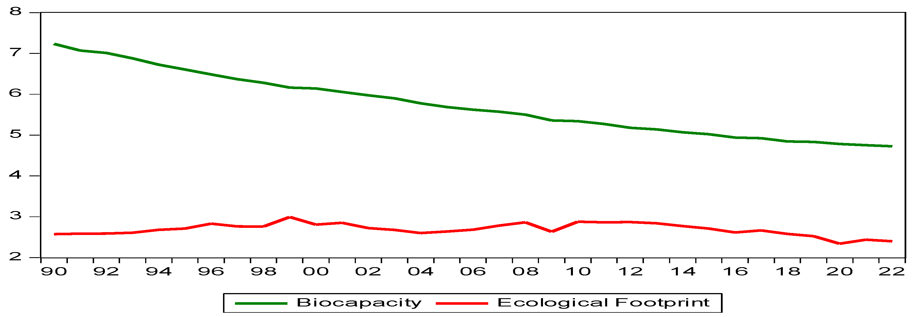
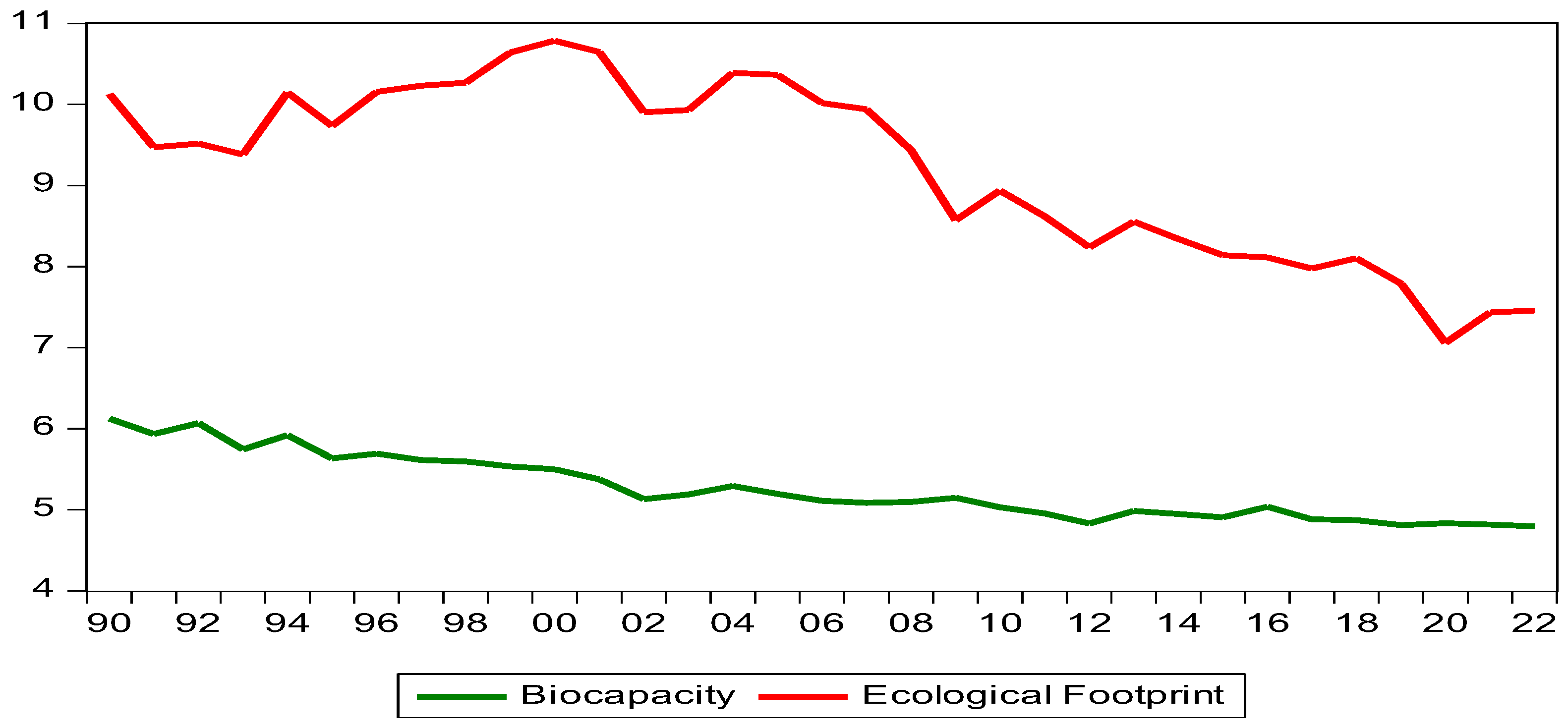
3. Results and Discussion

To test stochastic conditional convergence, the Dickey–Fuller (DF) [74] or Augmented Dickey–Fuller (DFA), Zivot–Andrews [75] with a structural change, and Lee–Strazicich [59] with two structural changes unit root tests were applied. Following Carlino and Mills [38], in this research, to test the convergence of the variables, the average of each variable is calculated annually by country, and then the relative natural logarithm of each variable is applied to each country. If there is a unit root, it implies that shock on the series would have a permanent effect (it does not return to its mean value), and, therefore, the hypothesis of stochastic conditional convergence would not be supported [38]. For energy consumption (

Table 1. Result of unit root tests for Enercon (1990–2022).

Enercon	DF or DFA Test C/CT	Zivot–Andrews Test One Break		Lee–Strazicich Test Two Breaks
		Crash	Break	Crash	Break
Argentina	−1.527/−1.850	−3.015 (2006)	−3.149 (2006)	−3.874 ** (2003, 2005)	−7.773 *** (2002, 2007)
Brazil	−0.323/−1.766	−3.539 (2007)	−3.528 (2008)	−2.788 (2007, 2013)	−6.521 ** (2006, 2014)
Chile	−2.239/−1.973	−2.998 (1996)	−2.999 (1996)	−4.112 *** (2013, 2017)	−5.773 (2001, 2013)
Canada	−1.733/−3.740 **	−5.042 ** (2016)	−5.516 ** (2010)	−4.462 ***(2006, 2015)	−7.062 *** (2007, 2014)
Colombia	−1.123/−1.514	−3.874 (2013)	−4.156 (1999)	−4.627 *** (2008, 2012)	−13.314 *** (2002, 2011)
Mexico	−1.601/−1.729	−3.061 (2001)	−3.111 (2001)	−4.124 *** (2010, 2019)	−5.258 (2001, 2013)
USA	−0.720/−1.789	−2.801 (2011)	−3.288 (2011)	−2.546 (2002, 2018)	−5.196 (2001, 2010)

*** and ** denote a rejection of the null hypothesis at 1 and 5% levels, respectively. The authors’ calculation is made using EViews 10.

), only Canada shows evidence in the three convergence tests in this variable. Argentina, Canada, and Colombia show evidence of conditional convergence when two structural changes are incorporated into the two models. Mexico and Chile show evidence of convergence with the Crash model, and Brazil with the Break model. However, the USA would have divergence since the series is not stationary or does not tend to return to its mean.

Regarding CO₂ emissions (

Table 2. Result of unit root tests for CO₂ (1990–2022).

CO2	DF or DFA Test C/CT	Zivot–Andrews Test One Break		Lee–Strazicich Test Two Breaks
		Crash	Break	Crash	Break
Argentina	−1.060/−2.111	−3.627 (2006)	−3.293 (2006)	−4.749 *** (2003, 2010)	−5.624 (2002, 2017)
Brazil	−1.081/−1.739	−3.005 (2010)	−3.547 (2012)	−3.379 ** (2001, 2016)	−6.677 ** (2003, 2018)
Chile	−1.136/−1.852	−4.224 (2011)	−4.147 (2011)	−5.104 *** (2003, 2010)	−6.733 ** (2005, 2013)
Canada	−3.233 **/−3.222 **	−4.275 (2000)	−4.142 (2000)	−4.489 *** (2006, 2011)	−5.785 (2005, 2010)
Colombia	−0.930/−1.209	−3.485 (1999)	−4.257 (2009)	−4.093 *** (2007, 2010)	−4.414 (2004, 2018)
Mexico	−2.564/−2.596	−3.652 (2002)	−3.841 (2009)	−3.612 ** (2003, 2006)	−5.998 * (2009, 2018)
USA	−0.462/−2.924	−4.976 (2011) **	−2.842 (2000)	−3.097 (2011, 2016)	−7.525 *** (2004, 2009)

***, **, and * denote a rejection of the null hypothesis at 1, 5, and 10% levels, respectively. The authors’ calculation is made using EViews 10.

), the most significant evidence of rejecting the unit root null hypothesis is when two structural changes are incorporated into the Crash model. There is convergence for Argentina, Brazil, Chile, Canada, Colombia, and Mexico. For the Break model, there is convergence for Brazil, Chile, Mexico, and The USA.

There is greater convergence when the ecological footprint is considered in the Crash model (

Table 3. Result of unit root tests for Ecologf (1990–2022).

Ecologf	DF or DFA Test C/CT	Zivot–Andrews Test One Break		Lee–Strazicich Test Two Breaks
		Crash	Break	Crash	Break
Argentina	−3.087 **/−3.417 *	−4.499 (1997)	−5.178 ** (2006)	−3.968 ** (2008, 2015)	−8.003 *** (2003, 2008)
Brazil	−1.782/−1.928	−3.870 (2008)	−3.999 (2008)	−3.412 * (2007, 2011)	−8.266 *** (2003, 2009)
Chile	−1.630/−2.593	−4.927 ** (1997)	−4.353 (1997)	−5.203 *** (2001, 2010)	−4.342 (2000, 2010)
Canada	−3.520 **/−4.054 **	−5.409 *** (1999)	−5.449 ** (2007)	−3.812 ** (2000, 2012)	−5.630 (2000, 2013)
Colombia	−1.830/−1.895	−4.046 (1999)	−4.487 (1999)	−4.332 *** (2001, 2011)	−4.758 (2003, 2008)
Mexico	−3.548 **/−3.537 **	−3.125 (1997)	−3.422 (2009)	−3.464 * (2003, 2012)	−10.291 *** (2002, 2010)
USA	−1.107/−2.160	−4.556 (2010)	−4.325 (2010)	−3.286 (2009, 2013)	−5.023 (2005, 2008)

***, **, and * denote a rejection of the null hypothesis at 1, 5, and 10% levels, respectively. The authors’ calculation is made using EViews 10.

). The presence of a unit root can be rejected in all countries except the USA. The six countries have convergence in environmental degradation per capita measured via the ecological footprint.

The Crash model with two structural changes presents evidence of convergence in energy intensity for all countries. In contrast, considering the Break model, there is evidence of convergence in Argentina, Brazil, Chile, Colombia, and Mexico (

Table 4. Result of unit root tests for Energyint (1990–2022).

Energyint	DF or DFA Test C/CT	Zivot–Andrews Test One Break		Lee–Strazicich Test Two Breaks
		Crash	Break	Crash	Break
Argentina	−0.634/−2.730	−3.793 (2002)	−3.811 (2002)	−4.856 *** (2005, 2011)	−9.674 *** (2000, 2008)
Brazil	−0.458/−3.500 *	−4.211 (2010)	−5.247 ** (2014)	−4.954 *** (2009, 2015)	−6.448 *** (2006, 2012)
Chile	−2.756 */−6.048 ***	−4.776 * (1997)	−4.562 (2003)	−5.850 *** (2006, 2009)	−6.372 ** (2009, 2015)
Canada	−0.682/−1.974	−5.013 ** (2016)	−4.694 (2016)	−3.434 * (2006, 2009)	−4.468 (2005, 2013)
Colombia	−2.458/−2.483	−7.270 *** (2013)	−6.450 (2013)	−4.175 *** (2010, 2012)	−11.809 *** (2003, 2011)
Mexico	−1.258/−3.110	−4.416 (2014)	−5.212 ** (2008)	−5.175 *** (2000, 2002)	−6.888 *** (2005, 2013)
USA	0.619/−2.672	−4.667 * (2007)	−5.320 ** (2007)	−3.336 * (2011, 2018)	−5.305 (2005, 2017)

***, **, and * denote a rejection of the null hypothesis at 1, 5, and 10% levels, respectively. The authors’ calculation is made using EViews 10.

).

Finally, considering the Locf indicator, the results show convergence for the seven countries considering the Crash model. In contrast, for the Break model, there is only convergence for Brazil, Chile, Canada, Colombia, and Mexico (

Table 5. Result of unit root tests for Locf (1990–2022).

Locf	DF or DFA Test C/CT	Zivot–Andrews Test One Break		Lee–Strazicich Test Two Breaks
		Crash	Break	Crash	Break
Argentina	−2.616/−2.717	−4.218 (1997)	−4.996 * (1999)	−3.642 ** (2008, 2012)	−4.665 (2010, 2017)
Brazil	−1.636/−3.330 *	−4.298 (2011)	−4.685 (2011)	−4.550 ** (2008, 2015)	−7.818 ** (2003, 2007)
Chile	−2.741 */−3.896 **	−4.661 * (1999)	−4.739 (2004)	−4.155 *** (2008, 2014)	−5.925 * (2000, 2013)
Canada	−2.554/−2.610	−4.824 * (1999)	−5.331 ** (2007)	−4.727 *** (2000, 2009)	−6.583 *** (2001, 2009)
Colombia	−2.344/−2.693	−3.889 (2016)	−4.511 (2012)	−4.553 *** (2013, 2019)	−5.590 *(2000, 2008)
Mexico	−3.282 **/−3.306 *	−3.583 (1997)	−4.552 * (1999)	−3.900 ** (2010, 2012)	−13.829 * (2006, 2012)
USA	−0.205/−1.867	−5.925 *** (2008)	−4.009 (2008)	−3.683 ** (2003, 2019)	−5.711 (2002, 2010)

***, **, and * denote a rejection of the null hypothesis at 1, 5, and 10% levels, respectively. The authors’ calculation is made using EViews 10.

). Therefore, considering the Crash model with two structural changes for a better specification, the majority of countries present evidence of convergence in energy consumption (six countries), CO₂ emissions (six countries), ecological footprint (six countries), energy intensity (all countries), and the Locf (all countries). In the case of the United States, there is no conclusive evidence of convergence in any of the indicators used. The countries of the Americas are very heterogeneous in terms of economic development, energy use, and environmental challenges, especially in the case of the United States.

In panel data analysis, it is essential to test the presence or absence of cross-sectional dependence in the data and, depending on this, to use suitable tests, making more appropriate statistical inferences. In this sense, CSD tests were applied: Breusch–Pagan [76] LM, Pesaran [77] scaled LM, Baltagi et al. [78] bias-corrected scaled LM, and Pesaran [77] CD. The null hypothesis of all four tests is that there is no cross-sectional dependence. In

Table 6. Results of CSD tests.

Tests	Enercon	CO2	Ecologf	Energyint	Locf
Breusch–Pagan LM	250.725 ***	219.456 ***	134.365 ***	280.055 ***	121.463 ***
Pesaran scaled LM	34.365 ***	29.542 ***	16.412 ***	38.892 ***	14.421 ***
Bias-corrected scaled LM	34.257 ***	29.433 ***	16.303 ***	38.783 ***	14.312 ***
Pesaran CD	−3.044 ***	0.480	−2.654 ***	−4.053 ***	−4.076 ***

*** denotes rejecting the null hypothesis at a 1% level. The authors’ calculation is made using EViews 10.

, the results show that the null hypothesis is rejected at a 1% significance level in the five variables and with the four tests, except for the Pesaran CD test for CO₂. Therefore, it is concluded that there is cross-sectional dependence in the variables for all the variables. Due to the above, the Im–Pesaran–Shin (IPS) [79], cross-sectional ADF (CADF), and IPS (CIPS) tests proposed by Pesaran [80], and the KT test proposed by Karavias and Tzavalis [58] were applied.

The results of the unit root tests are presented in

Table 7. Results of the stochastic convergence test.

Variable	IPS	CIPS	CADF	KT (1 Break)	KT (2 Breaks)
Enercon	0.600	−2.082	−2.126	−0.768	−1.101
CO2	0.088	−2.514	−2.115	−0.629	−1.909 ***
Ecologf	−2.486 ***	−3.532 ***	−2.907 **	−6.062 ***	−6.185 ***
Energyint	0.824	−2.128	−1.713	−1.505 ***	−1.798 ***
Locf	−2.023 **	−2.158 **	−1.985	−5.595 ***	−6.094 ***

*** and ** reject the null hypothesis at 1 and 5% levels, respectively. The authors’ calculation is made using Stata 16.0.

. In the case of energy consumption, the presence of a unit root is not rejected, so there is no evidence of convergence, considering the four tests applied. In the case of CO₂, considering two structural changes, it is possible to reject the null hypothesis of the unit root. The Ecologf is the only variable that rejects the null hypothesis of a unit root in all tests applied at 5% (or better). The series is stationary and tends to return to its mean. It implies convergence in environmental degradation measured by the ecological footprint per capita in the sample countries. Considering one and two endogenously determined structural changes, the Energyint is stationary. In the case of Locf, there is evidence of convergence with the IPS, CIPS, and KT (one and two breaks) tests. Therefore, there is evidence of stochastic convergence in CO₂, Ecologf, Energyint, and Locf in these countries. According to the literature, this convergence is conditional stochastic [38,43,81]. However, it is possible that with the panel data unit root tests applied, not all countries analyzed converge in the five indicators. It would be interesting to study whether there are any convergence clubs.

The results of the club convergence test are presented below to confirm the robustness. In this paper, a convergence club means that two or more countries are converging on the transition path of the indicator analyzed. A divergent group means that one or more countries are not converging on the transition path of the indicator analyzed. In

Table 8. Log t results of convergence test.

Variable	Coefficients	Standard Error	Statistic T	R
Enercon	−0.990	0.005	−179.355 *	0.3
CO2	−1.110	0.008	−134.508 *	0.3
Ecologf	−1.050	0.016	−62.546 *	0.3
Energyint	−1.159	0.006	−167.114 *	0.3
Locf	−0.879	0.004	−187.596 *	0.3

There are seven countries and 33 periods. * indicates rejection of the null hypothesis (convergence) at a 5% significance level.

, the results of the full panel test show evidence that there is no common long-term trend among the seven countries in energy consumption, CO₂ emissions, ecological footprint, energy intensity, and Locf; that is, there is no evidence of convergence in these variables for the countries in the sample.

Given the above, testing or analyzing the possibility of clubs or convergence groups for each variable analyzed is essential. The results of the grouping procedures and club merger tests for the seven countries are as follows.

Considering energy consumption, evidence of the convergence of two clubs and a divergent group is found. Chile, Canada, and the United States are in club 1, considering that the last two are developed countries based on a productive structure with high energy consumption per capita. Although Chile is not a developed country, it is one of the largest energy consumers in Latin America. In club 2 are Argentina, Brazil, and Mexico, while Colombia is divergent (

Table 9. Initial convergence club classification (Enercom).

Variable	Countries	Coefficient	T-Stat
Club 1	Canada, Chile, United States	0.005	13.076
Club 2	Argentina, Brazil, Mexico	0.229	3.300
Group (divergent)	Colombia	-	-

The null hypothesis is that there is convergence. The authors’ calculation is made using Stata 16.0.

).

The convergence trend of each club can be seen in Figure 5. There is no evidence of the possibility of the existence of additional clubs, according to the club fusion test (

Table 10. Club merging classification test (Enercom).

Variable	Coefficients	Standard Error	T-Stat
Club 1 + Club 2	−1.3042	0.0221	−58.933 *
Club 2 + Club 3	−0.411	0.0674	−6.109 *

* indicates rejection of the null hypothesis (convergence) at a 5% significance level. The authors’ calculation is made using Stata 16.0.

).

Considering CO₂ emissions, there is evidence of convergence in a club comprising Argentina, Canada, Chile, Mexico, and the United States and a divergent group comprising Brazil and Colombia (

Table 11. Initial convergence club classification (CO₂).

Variable	Countries	Coefficients	T-Stat
Club 1	Argentina, Canada, Chile, Mexico, United States	0.206	11.616 *
Group (divergent)	Brazil, Colombia	−1.233	−11.974

* Indicates rejection of the null hypothesis (convergence) at a significance level of 5%. The authors’ calculation using Stata 16.0.

). There is no evidence of the existence of additional clubs.

Figure 6 shows club 1’s convergence trend. According to this indicator, the United States and Canada, which have very similar paths, are the two economies on this continent with the highest pollution levels. However, both countries tend to converge in the long term with Argentina, Chile, and Mexico.

Regarding the ecological footprint, there is evidence of two clubs of convergence. In club 1, Argentina, Brazil, Canada, Chile, and the United States are the most polluting countries with this indicator (led by the United States and Canada). At the same time, Colombia and Mexico are in club 2 (

Table 12. Initial convergence club classification (Ecologf).

Variable	Countries	Coefficients	T-Stat
Club 1	Argentina, Brazil, Canada, Chile, United States	2.240	23.990
Club 2	Colombia, Mexico	1.463	6.026

The null hypothesis is that there is convergence. The author’s calculations were performed in Stata 16.0.

).

There is no evidence of the existence of additional clubs (

Table 13. Club merging classification test (Ecologf).

Variable	Coefficients	Standard Error	T-Stat
Club 1 + Club 2	−1.050	0.0168	−62.546

The null hypothesis is that there is convergence. The author’s calculations were performed in Stata 16.0.

), and Figure 7 shows the trend of each club’s convergence path.

In the case of energy intensity, there is evidence of a convergence club and a divergent group (

Table 14. Initial convergence club classification (Energyint).

Variable	Countries	Coefficients	T-Stat
Club 1	Brazil, Canada, United State	0.206	11.616
Group (divergent)	Argentina, Chile, Colombia, Mexico	−1.233	−11.974 *

* indicates rejection of the null hypothesis (convergence) at a significance level of 5%. The authors’ calculation using Stata 16.0.

). Brazil, Canada, and the United States are the convergence club 1 with the highest energy intensity levels, while Argentina, Chile, Colombia, and Mexico are the divergent group.

There is no evidence of additional clubs, and Figure 8 shows the trend of club 1’s convergence paths.

Finally, considering the case of Locf, there is evidence of convergence of two clubs and a divergent group. Brazil and Canada are in club 1, assuming they have the most natural resources and are above the sustainability limit. In club 2 are Chile, Mexico, and the USA, countries below the sustainability limit. Finally, Argentina and Colombia are within the divergent group above the sustainability limit (

Table 15. Initial convergence club classification (Locf).

Variable	Countries	Coefficient	T-Stat
Club 1	Brazil and Canada	0.076	0.984
Club 2	Chile, Mexico, and USA	0.194	3.760
Group (divergent)	Argentina and Colombia	−0.479	−11.788

The null hypothesis is that there is convergence. The authors’ calculation is made using Stata 16.0.

).

Figure 9 shows each club’s convergence trend. Club 1 shows an important gap between Brazil and Canada but tends to reduce and converge in the long term. Club 2 shows a clear trend towards convergence in the long term. Mexico’s and the USA’s trends are very similar, which could explain the solid commercial integration between both countries.

According to the club fusion test, there is no evidence of the possibility of additional clubs (

Table 16. Club merging classification test (Locf).

Variable	Coefficients	Standard Error	T-Stat
Club 1 + Club 2	−0.947	0.017	−54.700 *
Club 2 + Group 3	−0.429	0.027	−15.377 *

* indicates rejection of the null hypothesis (convergence) at a 5% significance level. The authors’ calculation is made using Stata 16.0.

).

Considering that the Locf is the most complete indicator to measure environmental degradation, according to the results, the countries could be classified into two clubs and a divergent group. In the first club, Brazil and Canada are the countries with the highest level of sustainability and biocapacity reserves in the Americas. In the divergent group of countries, Argentina and Colombia, representing some countries still above the sustainability limit, but whose biocapacity reserves and sustainability tend to decrease. Finally, in the second club are the United States, Mexico, and Chile, which are countries that are below the sustainability line, so the current lifestyle or environmental condition of these countries is unsustainable, and thus there is a biocapacity deficit.

Next, studying the possible drivers of forming convergence clubs is crucial. In this sense, logit models are estimated to investigate the variables expected to influence the probability of a country being in a specific convergence club for energy consumption, carbon dioxide emissions, ecological footprint, and energy intensity. According to the literature review, the main explanatory variables in the convergence are economic growth, trade openness, renewable energy consumption, income inequality, and innovative activity.

Table 17. Determinants of convergence clubs (Enercom).

	Club 1		Club 2
Variable	Odds Ratio	Marginal Effects dy/dx	Odds Ratio	Marginal Effects dy/dx
GDP	0.131 ***	−0.465 **	1.782 **	0.137 **
Patent	14.007 ***	0.633 ***	0.461 ***	−0.183 ***
Renergy	2.505 ***	0.210 ***	0.443 ***	−0.193 ***
Tradeopen	280.788 ***	1.294 ***	0.095 ***	−0.559 ***
	Wald chi2 = 100.39 Prob (0.000)		Wald chi2 = 74.91 Prob (0.000)

*** and ** indicate rejection of the null hypothesis at a significance level of 1 and 5%, respectively. The authors’ calculation is made using Stata 16.0.

shows the odds ratios and marginal effects for Enercom. In club 1, innovative activity, renewable energy, and trade increase countries’ probability of belonging to this specific club, while economic activity reduces the probability. In club 2, economic activity has a positive marginal effect, while the other variables have a negative sign.

The results for CO₂ are shown in

Table 18. Determinants of convergence clubs (CO₂).

	Club 1
Variable	Odds Ratio	Marginal Effects dy/dx
GDP	5.589 ***	0.123 **
Patent	0.456 ***	−0.056 **
Gini	4.42 × 10−7 ***	−1.050 *
Tradeopen	93.268 ***	0.325 ***
	Wald chi2 = 119.67 Prob (0.000)

***, **, and * indicate rejection of the null hypothesis at a significance level of 1, 5, and 10%, respectively. The authors’ calculation is made using Stata 16.0.

. There is only one convergence club; economic activity and trade increase the probability of countries belonging, while inequality and innovative activity reduce it.

Two convergence clubs were found when using the ecological footprint as an indicator of environmental degradation (

Table 19. Determinants of convergence clubs (Ecologf).

	Club 1		Club 2
Variable	Odds Ratio	Marginal Effects dy/dx	Odds Ratio	Marginal Effects dy/dx
GDP	0.336 ***	−0.046 **	2.795 ***	0.046 **
Gini	41.384 **	0.159 *	0.024 **	−0.159 *
Patent	12.049 ***	0.106 **	0.082 ***	−0.106 **
Renergy	5.153 ***	0.070 ***	0.194 ***	−0.070 ***
Tradeopen	0.215 **	−0.066 ***	4.647 **	0.066 ***
	Wald chi2 = 41.43 Prob (0.000)		Wald chi2 = 29.35 Prob (0.000)

***, **, and * indicate rejection of the null hypothesis at a significance level of 1, 5, and 10%, respectively. The authors’ calculation is made using Stata 16.0.

). In club 1, income inequality, innovative activity, and renewable energy consumption have positive marginal effects on probability, while economic activity and trade reduce it. In club 2, economic activity and trade increase the probability of countries belonging, while the other variables reduce it.

Table 20. Determinants of convergence clubs (Energyint).

	Club 1
Variable	Odds Ratio	Marginal Effects dy/dx
GDP	12.974 ***	0.555 ***
Gini	5.45 × 10−7 ***	−3.126 ***
Tradeopen	0.009 ***	−1.003 ***
	Wald chi2 = 73.70 Prob (0.000)

*** indicates rejection of the null hypothesis at a significance level of 1%. The authors’ calculation is made using Stata 16.0.

shows the results for energy intensity. There is only one convergence club; economic activity increases the probability of countries belonging, while inequality and trade reduce it.

Using the Locf as an indicator of environmental degradation, two convergence clubs were found (

Table 21. Determinants of convergence clubs (Locf).

	Club 1		Club 2
Variable	Odds Ratio	Marginal Effects dy/dx	Odds Ratio	Marginal Effects dy/dx
GDP	0.917 **	−0.015 **	0.717 ***	−0.076 ***
Renergy	5.240 ***	0.304 ***	0.046 ***	−0.708 ***
Tradeopen	0.376 ***	−0.179 ***	11.713 ***	0.565 ***
Gini	--	--	9.475 ***	0.517 ***
	Wald chi2 = 54.61 Prob (0.000)		Wald chi2 = 41.54 Prob (0.000)

*** and ** indicate rejection of the null hypothesis at a significance level of 1 and 5%, respectively. Source: The authors’ calculation using Stata 16.0.

). In club 1, renewable energy consumption has positive marginal effects on probability, while economic activity and trade reduce it. In club 2, trade increases the probability of countries belonging, while economic activity and renewable energy consumption reduce it.

Next, the cross-sectional dependence, unit root, and cointegration tests will be applied, as well as the long-term estimation of the parameters, to see the influence of each variable on the environmental degradation measured by Locf.

Table 22. Results of CSD tests for long-run model.

Tests	GDP	Gini	Locf	Patents	Renergy	Tradeopen
Breusch–Pagan LM	610.317 ***	283.064 ***	276.780 ***	358.044 ***	94.849 ***	160.935 ***
Pesaran scaled LM	89.853 ***	39.357 ***	38.387 ***	50.926 ***	10.315 ***	20.512 ***
Bias-corrected scaled LM	89.736 ***	39.240 ***	38.271 ***	50.810 ***	10.198 ***	20.395 ***
Pesaran CD	24.698 ***	5.623 ***	12.978 ***	16.044 ***	1.996 **	11.221 ***

*** and ** indicate rejection of the null hypothesis at a significance level of 1 and 5%, respectively. Source: The authors’ calculation using EViews 10.

presents the results of the tests, where all variables reject the null hypothesis of no cross-sectional dependence.

Given the above, Pesaran’s [80] CIPS unit root test will be applied. The unit root test results indicate that the variables in levels present a stochastic trend but are stationary in first differences and integrated of order one (

Table 23. Results of the unit root and cointegration tests.

Variables	CIPS (Levels)	CIPS (First Difference)
GDP	−1.610	−3.621 ***
Gini	−1.544	−3.002 ***
Locf	−1.954	−5.134 ***
Patents	−2.531	−5.638 ***
Renergy	−2.126	−5.002 ***
Tradeopen	−2.149	−4.293 ***
	Cointegration test Kao [82]	Cointegration test Westerlund [68]
	Statistic−4.420 ***	Statistic−1.816 **

*** and ** reject the null hypothesis at 1 and 5% levels, respectively. The authors’ calculation is made using Stata 16.0.

). Kao [82] and Westerlund [68] cointegration tests are applied in this sense. The results at the bottom of Table 23 indicate that the hypothesis of non-cointegration of both tests is rejected at a 1 and 5% significance level, respectively. It implies that there is a long-term equilibrium relationship between the variables. Although each of the variables separately has a stochastic tendency, in the long term, there is a convergence towards equilibrium. Because there is cross-sectional dependence between the variables, the FGLS and PCSE methods will be applied to estimate the long-term parameters.

The results show evidence (

Table 24. Long-term model.

Variables	FGLS Coefficients	PCSE Coefficients
GDP	−0.116 ***	−0.099 **
Gini	−2.224 ***	−2.701 ***
Patents	−0.074 ***	−0.106 ***
Renergy	0.824 ***	0.873 ***
Tradeopen	−0.838 ***	−0.992 ***

*** and ** denote the rejection of the null hypothesis at the 1 and 5% levels, respectively. The authors’ calculation is made using Stata 16.0.

) of a negative influence of economic activity, income inequality, innovative activity (in general), and trade openness on sustainability. As expected, greater economic activity requires greater energy consumption and greater environmental degradation. These results are similar to those found by Caglar et al. [19] for APEC countries, by Djedaiet et al. [20] for the APEC oil countries, and by Dogan and Pata [21] for the G7. The greater the inequality in wealth distribution, the greater the environmental deterioration, especially in most of the selected Latin American countries. These results are similar to those found by Khan et al. [32] for Asian developing economies and Ehigiamusoe et al. [31] for different countries’ income levels. Innovative activity, in general, is not enough to improve the environment; these results coincide with Cheng et al. [23] for OECD countries and Allard et al. [83] for 74 countries. Likewise, greater trade openness negatively affects the sustainability of the selected countries of the American continent. These results are similar to those found by Allard et al. [83] for 74 countries. Evidence shows that renewable energy will improve environmental sustainability in the region. These results are similar to those of Caglar et al. [19] for APEC countries.

Table 25. Causality test results.

Variables	GDP	Gini	Locf	Patents	Renergy	Tradeopen
GDP	-	−0.740	−0.410	−2.480 **	−1.310	6.910 ***
Gini	−2.090 ***	-	−3.760 ***	0.700	1.590	−4.020 ***
Locf	−3.980 ***	0.350	-	1.190	2.97 ***	−7.700 ***
Patents	2.240 **	5.920 ***	0.630	-	−1.60	1.260
Renergy	−0.110	−0.880	2.510 **	4.440 ***	-	−2.060 **
Tradeopen	2.100 **	0.990	−0.370	−1.680 **	−0.270	-

*** and ** denote the rejection of the null hypothesis at the 1 and 5% levels, respectively. The authors’ calculation is made using Stata 16.0.

presents the results of the causality test. There is evidence of a bidirectional causal relationship between renewable energy and environmental degradation, between economic activity and trade openness, and between economic activity and patenting activity. Each of these variables contains important information that helps to better predict the behavior of the other variable. It highlights the direction of unidirectional causality from economic activity, renewable energy, and trade openness to environmental degradation. Any movement in these variables affects the sustainability of these countries, that is, greater economic activity and greater trade openness reduce it, while greater use of renewable energy increases it. This information is relevant for the energy transition of these countries.

4. Conclusions and Policy Implications

This paper studies the convergence of environmental sustainability and its main determinants in selected countries of the Americas for the period 1990–2022. Furthermore, this paper studies the effect of economic activity, income inequality, trade openness, and innovative activity on sustainability. Cross-sectional dependence, unit root, club convergence, causality, and cointegration tests are applied. In addition, long-term parameters are estimated using robust methods for cross-sectional dependence, such as FGLS and PCSE. The results show evidence of stochastic convergence with the univariate unit root tests in the five indicators used (Enercon, CO₂, Ecologf, Energyint, and Locf); although, in the case of the United States, there is no conclusive evidence of convergence in all the indicators used, while with the unit root tests of panel data, there is only convergence in four indicators (CO₂, Ecologf, Energyint, and Locf). Furthermore, there is no evidence of convergence towards a single club considering the entire sample, but there is evidence of convergence towards several clubs. In the case of energy consumption, two clubs were found, for CO₂ emissions one club, for the ecological footprint two clubs, for energy intensity one club, and for the Locf two clubs. The results suggest that the variables are integrated of order one and are cointegrated in the long run. In the long term, economic activity, income inequality, trade openness, and innovative activity deteriorate sustainability, while renewable energy improves the sustainability of these countries. There is evidence of a bidirectional causal relationship between renewable energy and environmental degradation, between economic activity and trade openness, and between economic activity and patenting activity. Furthermore, the direction of unidirectional causality from economic activity, renewable energy, and trade openness to environmental degradation confirms that greater economic activity and trade openness reduce sustainability, while greater use of renewable energy increases sustainability. This information is relevant for the energy transition of these countries. It implies accelerating this region’s transition from fossil energy sources to renewable and cleaner energy. The countries could be classified into two clubs and one group, considering the convergence results of the Locf indicator, to design and implement specific energy and environmental policies. In the first club, Brazil and Canada are the countries with the highest levels of sustainability, so environmental and energy policies should be aimed at maintaining and increasing sustainability levels. In the divergent group of countries, Argentina and Colombia, although they are above the sustainability limit, sustainability tends to decrease, so specific environmental and energy policies are necessary to move away from the limit and converge towards greater sustainability. Finally, in the second club are the United States, Mexico, and Chile, where the current lifestyle or environmental condition is unsustainable. Specific environmental and energy policies are urgently needed for these countries to move to a sustainable environmental condition. According to the results of the long-term model, it is important to consider that the energy and environmental policies of these countries should focus on promoting economic activities that reduce energy intensity, reduce income inequality, promote green patents, and encourage the production and use of renewable and cleaner energy sources.

Regarding the limitations of the study, one of them is the sample period; it is always desirable to have a greater number of observations. In addition to the fact that it was not possible to find data for all the countries of the Americas, complete data on the variables used were only available for seven countries, which were the main consumers of energy and those that generate the most environmental pollution. Also, although robust methodologies were included to address the heterogeneity and cross-section dependence between the countries considered, this may be an element to take into account.

References

1. UNFCCC. The Paris Agreement, United Nations. 2015. Available online: https://unfccc.int/process-and-meetings/the-paris-agreement (accessed on 5 July 2023).
2. Guo, Q.; Ahmad, W.; Sofuoğlu, E.; Abbas, S. Testing the equity-pollution dilemma from a global perspective: Does reducing consumption inequality impose environmental burdens? Gondwana Res. 2023, 122, 125–137. [Google Scholar] [CrossRef]
3. Panayotou, T. Technology and Employment Program. In Empirical Tests and Policy Analysis of Environmental Degradation at Different Stages of Economic Development; Working Paper WP238; International Labour Office: Geneva, Switzerland, 1993; pp. 1–42. [Google Scholar]
4. Altıntaş, H.; Kassouri, Y. Is the environmental Kuznets Curve in Europe related to the per-capita ecological footprint or CO2 emissions? Ecol. Indic. 2020, 113, 106187. [Google Scholar] [CrossRef]
5. Awad, A. Is there any impact from ICT on environmental quality in Africa? Evidence from second-generation panel techniques. Environ. Chall. 2020, 7, 100520. [Google Scholar] [CrossRef]
6. Aydin, M.; Degirmenci, T.; Gurdal, T.; Yavuz, H. The role of green innovation in achieving environmental sustainability in European Union countries: Testing the environmental Kuznets curve hypothesis. Gondwana Res. 2023, 118, 105–116. [Google Scholar] [CrossRef]
7. Kalim, R.; Ul-Durar, S.; Iqbal, M.; Arshed, N.; Shahbaz, M. Role of knowledge economy in managing demand-based Environmental Kuznets Curve. Geosci. Front. 2023, 15, 101594. [Google Scholar] [CrossRef]
8. Karimi, M.; Khezri, M.; Khan, Y.A.; Somayeh, R. Exploring the influence of economic freedom index on fishing grounds footprint in environmental Kuznets curve framework through spatial econometrics technique: Evidence from Asia-Pacific countries. Environ. Sci. Pollut. Res. 2022, 29, 6251–6266. [Google Scholar] [CrossRef] [PubMed]
9. Nizamani, R.A.; Shaikh, F.; Nizamani, A.G.; Mirjat, N.H.; Kumar, L.; Assad, M.E.H. The impacts of conventional energies on environmental degradation: Does Pakistan’s economic and environmental model follow the Kuznets curve? Environ. Sci. Pollut. Res. 2023, 30, 7173–7185. [Google Scholar] [CrossRef]
10. Sesma-Martín, D.; Puente-Ajovín, M. The Environmental Kuznets Curve at the thermoelectricity-water nexus: Empirical evidence from Spain. Water Resour. Econ. 2022, 39, 100202. [Google Scholar] [CrossRef]
11. Taghvaee, V.M.; Nodehi, M.; Saboori, B. Economic complexity and CO2 emissions in OECD countries: Sector-wise Environmental Kuznets Curve hypothesis. Environ. Sci. Pollut. Res. 2022, 29, 80860–80870. [Google Scholar] [CrossRef]
12. Wang, Q.; Yang, T.; Li, R. Does income inequality reshape the environmental Kuznets curve (EKC) hypothesis? A nonlinear panel data analysis. Environ. Res. 2023, 216, 114575. [Google Scholar] [CrossRef]
13. Dogan, E.; Ulucak, R.; Kocak, E.; Isik, C. The use of ecological footprint in estimating the Environmental Kuznets Curve hypothesis for BRICST by considering cross-section dependence and heterogeneity. Sci. Total Environ. 2020, 723, 138063. [Google Scholar] [CrossRef] [PubMed]
14. Wackernagel, M.; Monfreda, C.; Erb, K.H.; Haberl, H.; Schulz, N.B. Ecological footprint time series of Austria, the Philippines, and South Korea for 1961–1999: Comparing the conventional approach to an ‘actual land area’ approach. Land Use Policy 2004, 21, 261–269. [Google Scholar] [CrossRef]
15. Galli, A. On the rationale and policy usefulness of Ecological Footprint Accounting: The case of Morocco. Environ. Sci. Policy 2004, 48, 210–224. [Google Scholar] [CrossRef]
16. Pata, U.K.; Isik, C. Determinants of the load capacity factor in China: A novel dynamic ARDL approach for ecological footprint accounting. Resour. Policy 2021, 74, 102313. [Google Scholar] [CrossRef]
17. Global Footprint Network. Available online: https://www.footprintnetwork.org/our-work/ (accessed on 1 October 2023).
18. Siche, R.; Pereira, L.; Agostinho, F.; Ortega, E. Convergence of ecological footprint and emergy analysis as a sustainability indicator of countries: Peru as case study. Commun. Nonlinear Sci. Numer. Simulat. 2010, 15, 3182–3192. [Google Scholar] [CrossRef]
19. Caglar, A.E.; Pata, U.K.; Ulug, M.; Zafar, M.W. Examining the impact of clean environmental regulations on load capacity factor to achieve sustainability: Evidence from APEC economies. J. Clean. Prod. 2023, 429, 139563. [Google Scholar] [CrossRef]
20. Djedaiet, A.; Ayad, H.; Ben-Salha, O. Oil prices and the load capacity factor in African oil-producing OPEC members: Modeling the symmetric and asymmetric effects. Resour. Policy 2024, 89, 104598. [Google Scholar] [CrossRef]
21. Dogan, A.; Pata, U.K. The role of ICT, R&D spending and renewable energy consumption on environmental quality: Testing the LCC hypothesis for G7 countries. J. Clean. Prod. 2022, 380, 135038. [Google Scholar] [CrossRef]
22. Fang, Z.; Wang, T.; Yang, C. Nexus among natural resources, environmental sustainability, and political risk: Testing the load capacity factor curve hypothesis. Resour. Policy 2024, 90, 104791. [Google Scholar] [CrossRef]
23. Cheng, C.; Ren, X.; Wang, Z. The impact of renewable energy and innovation on carbon emission: An empirical analysis for OECD countries. Energy Procedia 2019, 158, 1506–1512. [Google Scholar] [CrossRef]
24. Alvarado, R.; Ponce, P.; Alvarado, R.; Ponce, K.; Huachizaca, V.; Toledo, E. Sustainable and non-sustainable energy and output in Latin America: A cointegration and causality approach with panel data. Energy Strat. Rev. 2019, 26, 100369. [Google Scholar] [CrossRef]
25. Wolde-Rufael, Y.; Mulat-Weldemeskel, E. The moderating role of environmental tax and renewable energy in CO2 emissions in Latin America and Caribbean countries: Evidence from method of moments quantile regression. Environ. Chall. 2022, 6, 100412. [Google Scholar] [CrossRef]
26. Vural, G. Analyzing the impacts of economic growth, pollution, technological innovation and trade on renewable energy production in selected Latin American countries. Renew. Energy 2021, 171, 210–216. [Google Scholar] [CrossRef]
27. Moreno, L.A. Prefacio. In La Crisis de la Desigualdad: América Latina y el Caribe en la Encrucijada; Busso, M., Messina, J., Eds.; Banco Interamericano de Desarrollo: Washington, DC, USA, 2020. [Google Scholar]
28. Boyce, J.K. Is Inequality Bad for the Environment? Res. Soc. Probl. 2008, 15, 267–288. [Google Scholar]
29. Ridzuan, S. Inequality and the environmental Kuznets curve. J. Clean. Prod. 2019, 228, 1472–1481. [Google Scholar] [CrossRef]
30. Stiglitz, J.E. Inequality and environmental policy. In Green Planet Blues: Critical Perspectives on Global Environmental Politics, 6th ed.; Dabelko, G.D., Ed.; Routledge: New York, NY, USA, 2019. [Google Scholar] [CrossRef]
31. Ehigiamusoe, K.U.; Majeed, M.T.; Dogan, E. The nexus between poverty, inequality and environmental pollution: Evidence across different income groups of countries. J. Clean. Prod. 2022, 341, 130863. [Google Scholar] [CrossRef]
32. Khan, S.; Yahong, W.; Zeeshan, A. Impact of poverty and income inequality on the ecological footprint in Asian developing economies: Assessment of Sustainable Development Goals. Energy Rep. 2022, 8, 670–679. [Google Scholar] [CrossRef]
33. Hailemariam, A.; Dzhumashev, R.; Shahbaz, M. Carbon emissions, income inequality, and economic development. Empir. Econ. 2020, 59, 1139–1159. [Google Scholar] [CrossRef]
34. Ockwell, D.G.; Haum, R.; Mallett, A.; Watson, J. Intellectual property rights and low carbon technology transfer: Conflicting discourses of diffusion and development. Glob. Environ. Change 2010, 20, 729–738. [Google Scholar] [CrossRef]
35. Töbelmann, D.; Wendler, T. The impact of environmental innovation on carbon dioxide emissions. J. Clean. Prod. 2020, 244, 118787. [Google Scholar] [CrossRef]
36. Baumol, W.J. Productivity Growth, Convergence, and Welfare: What the Long-Run Data Show. Am. Econ. Rev. 1986, 76, 1072–1085. Available online: http://www.jstor.org/stable/1816469 (accessed on 8 June 2024).
37. Barro, R.J.; Sala-i-Martin, X. Economic Growth and Convergence across the United States. NBER Work. Pap. 1990, 3419, 1–39. [Google Scholar]
38. Carlino, G.; Mills, L. Testing neoclassical convergence in regional incomes. Reg. Sci. Urban Econ 1996, 26, 565–590. [Google Scholar] [CrossRef]
39. Phillips, P.C.B.; Sul, D. Transition Modeling and Econometric Convergence Tests. J. Econom. Soc. 2007, 75, 1771–1855. Available online: https://www.jstor.org/stable/4502048 (accessed on 8 June 2024). [CrossRef]
40. Phillips, P.C.B.; Sul, D. Economic transition and growth. J. Appl. Econom. 2009, 24, 1153–1185. [Google Scholar] [CrossRef]
41. Mishra, V.; Smyth, R. Convergence in energy consumption per capita among ASEAN countries. Energy Policy 2014, 73, 180–185. [Google Scholar] [CrossRef]
42. Haider, S.; Akram, V. Club convergence analysis of ecological and carbon footprint: Evidence from a cross-country analysis. Carbon Manag. 2019, 10, 451–463. [Google Scholar] [CrossRef]
43. Meng, M.; Payne, J.E.; Lee, J. Convergence in per capita energy use among OECD countries. Energy Econ. 2013, 36, 536–545. [Google Scholar] [CrossRef]
44. Karakaya, E.; Alataş, S.; Yılmaz, B. Replication of Strazicich and List (2003): Are CO2 emission levels converging among industrial countries? Energy Econ. 2019, 82, 135–138. [Google Scholar] [CrossRef]
45. Romero-Ávila, D.; Tolga, O. Convergence of per capita energy consumption around the world: New evidence from nonlinear panel unit root tests. Energy Econ. 2022, 111, 106062. [Google Scholar] [CrossRef]
46. Kazemzadeh, E.; Fuinhas, J.A.; Koengkan, M.; Shadmehri, M.T.A. Relationship between the share of renewable electricity consumption, economic complexity, financial development, and oil prices: A two-step club convergence and PVAR model approach. Int. Econ. 2023, 173, 260–275. [Google Scholar] [CrossRef]
47. Vo, D.H.; Vo, L.H.; Ho, C.M. Regional convergence of nonrenewable energy consumption in Vietnam. Energy Policy 2022, 169, 113194. [Google Scholar] [CrossRef]
48. Simionescu, M. Stochastic convergence in per capita energy use in the EU-15 countries. The role of economic growth. Appl. Energy 2022, 322, 119489. [Google Scholar] [CrossRef]
49. He, W.; Chen, H. Will China’s provincial per capita energy consumption converge to a common level over 1990–2017? Evidence from a club convergence approach. Energy 2022, 249, 123624. [Google Scholar] [CrossRef]
50. Salman, M.; Zha, D.; Wang, G. Assessment of energy poverty convergence: A global analysis. Energy 2022, 255, 124579. [Google Scholar] [CrossRef]
51. Saba, C.S.; Ngepah, N. Convergence in renewable energy sources and the dynamics of their determinants: An insight from a club clustering algorithm. Energy Rep. 2022, 8, 3483–3506. [Google Scholar] [CrossRef]
52. Zhang, Y.; Jin, W.; Xu, M. Total factor efficiency and convergence analysis of renewable energy in Latin American countries. Renew. Energy 2021, 170, 785–795. [Google Scholar] [CrossRef]
53. Belloc, I.; Molina, J.A. Are greenhouse gas emissions converging in Latin America? Implications for environmental policies. Econ. Anal. Policy 2023, 77, 337–356. [Google Scholar] [CrossRef]
54. Tillaguango, B.; Alvarado, R.; Dagar, V.; Murshed, M.; Pinzón, Y.; Méndez, P. Convergence of the ecological footprint in Latin America: The role of the productive structure. Environ. Sci. Pollut. Res. 2021, 28, 59771–59783. [Google Scholar] [CrossRef]
55. Alvarado, R.; Tillaguango, B.; Cuesta, L.; Pinzon, S.; Alvarado-Lopez, M.R.; Işık, C.; Dagar, V. Biocapacity convergence clubs in Latin America: An analysis of their determining factors using quantile regressions. Environ. Sci. Pollut. Res. 2022, 29, 66605–66621. [Google Scholar] [CrossRef]
56. Martins, M.A.; Heshmati, A. Convergence of carbon dioxide emissions in the Americas and its determinants. Lat. Am. Econ. Rev. 2022, 31, 1–33. [Google Scholar] [CrossRef]
57. Gregory, A.W.; Hansen, B.E. Residual-based tests for cointegration in models with regime shifts. J. Econom. 1996, 70, 99–126. [Google Scholar] [CrossRef]
58. Karavias, Y.; Tzavalis, E. Testing for unit roots in short panels allowing for a structural break. Comput. Stat. Data Anal. 2014, 76, 391–407. [Google Scholar] [CrossRef]
59. Lee, J.; Strazicich, M.C. Minimum Lagrange Multiplier Unit Root Test with Two Structural Breaks. Rev. Econ. Stat. 2003, 85, 1082–1089. [Google Scholar] [CrossRef]
60. Perron, P. Further Evidence on Breaking Trend Functions in Macroeconomic Variables. J. Econom. 1997, 80, 355–385. [Google Scholar] [CrossRef]
61. Chen, P.; Karavias, Y.; Tzavalis, E. Panel Unit Root Tests with Structural Breaks; Discussion Papers 21-12; Department of Economics, University of Birmingham: Birmingham, UK, 2021. [Google Scholar]
62. Juodis, A.; Karavias, Y.; Sarafidis, V. A homogeneous approach to testing for Granger non-causality in heterogeneous panels. Empir. Econ. 2021, 60, 93–112. [Google Scholar] [CrossRef]
63. The Enerdata Yearbook. World Energy & Climate Statistics. Available online: https://www.enerdata.net (accessed on 25 July 2023).
64. World Bank. World Development Indicators. Available online: http://data.worldbank.org/ (accessed on 5 July 2023).
65. Solt, F. Measuring Income Inequality across Countries and Over Time: The Standardized World Income Inequality Database, SWIID Version 9.5. 2020. Available online: https://fsolt.org/swiid/ (accessed on 10 November 2023).
66. Baltagi, B.H. Econometric Analysis of Panel Data, 1st ed.; John Wiley and Sons: New York, NY, USA, 1995. [Google Scholar]
67. Ivanovski, K.; Churchill, S.A.; Smyth, R. A club convergence analysis of per capita energy consumption across Australian regions and sectors. Energy Econ. 2018, 76, 519–531. [Google Scholar] [CrossRef]
68. Westerlund, J. Testing for error correction in panel data. Oxf. Bull. Econ. Stat. 2007, 69, 709–748. [Google Scholar] [CrossRef]
69. Beck, N.; Katz, J.N. What to do (and not to do) with time series cross-section data. Am. Political Sci. Rev. 1995, 89, 634–647. [Google Scholar] [CrossRef]
70. Parks, R. Efficient estimation of a regression equation system when disturbances are serially and contemporaneously correlated. J. Am. Stat. Assoc. 1967, 62, 500–509. [Google Scholar] [CrossRef]
71. You, W.; Zhang, Y.; Lee, C.C. The dynamic impact of economic growth and economic complexity on CO2 emissions: An advanced panel data estimation. Econ. Anal. Policy 2022, 73, 112–128. [Google Scholar] [CrossRef]
72. Xiao, J.; Karavias, Y.; Juodis, A.; Sarafidis, V.; Ditzen, J. Improved tests for Granger noncausality in panel data. Stata J. 2023, 23, 230–242. [Google Scholar] [CrossRef]
73. Dumitrescu, E.I.; Hurlin, C. Testing for Granger non-causality in heterogeneous panels. Econ. Model. 2012, 29, 1450–1460. [Google Scholar] [CrossRef]
74. Dickey, D.A.; Fuller, W.A. Distribution of the Estimators for Autoregressive Time Series with a Unit Root. J. Am. Stat. Assoc. 1979, 74, 427–431. [Google Scholar] [CrossRef]
75. Zivot, E.; Andrews, W.K. Further evidence on the great crash, the oil-price shock, and the unit root hypothesis. J. Bus. Econ. Stat. 1992, 10, 251–270. [Google Scholar] [CrossRef]
76. Breusch, T.; Pagan, A. The Lagrange Multiplier Test and its Application to Model Specification in Econometrics. Rev. Econ. Stud. 1980, 47, 239–253. [Google Scholar] [CrossRef]
77. Pesaran, M.H. General Diagnostic Tests for Cross Section Dependence in Panels; Cambridge Working Papers in Economics No. 0435; Faculty of Economics, University of Cambridge: Cambridge, UK, 2004. [Google Scholar]
78. Baltagi, B.H.; Feng, Q.; Kao, C. A Lagrange Multiplier test for Cross-sectional Dependence in a Fixed Effects Panel Data Model. J. Econom. 2012, 170, 164–177. [Google Scholar] [CrossRef]
79. Im, K.S.; Pesaran, M.H.; Shin, Y. Testing for unit roots in heterogeneous panels. J. Econom. 2003, 115, 53–74. [Google Scholar] [CrossRef]
80. Pesaran, M.H. A simple panel unit root test in the presence of cross section dependence. J. Appl. Econom. 2007, 22, 265–312. [Google Scholar] [CrossRef]
81. Strazicich, M.C.; List, J.A. Are CO2 Emission Levels Converging Among Industrial Countries? Environ. Resour. Econ. 2003, 24, 263–271. [Google Scholar] [CrossRef]
82. Kao, C. Spurious Regression and Residual-Based Tests for Cointegration in Panel Data. J. Econom. 1999, 90, 1–44. [Google Scholar] [CrossRef]
83. Allard, A.; Takman, J.; Uddin, G.S.; Ahmed, A. The N-shaped environmental Kuznets curve: An empirical evaluation using a panel quantile regression approach. Environ. Sci. Pollut. Res. 2017, 25, 5848–5861. [Google Scholar] [CrossRef] [PubMed]
Figure 1. Ecological footprint and biocapacity in Latin America and the Caribbean. Source: Global Footprint Network [17].
Sustainability 16 06819 g001
Figure 2. Ecological footprint and biocapacity of North America. Source: Global Footprint Network [17].
Sustainability 16 06819 g002
Figure 3. Load capacity factor (Locf) for the leading countries of the Americas. Source: Global Footprint Network [17].
Sustainability 16 06819 g003
Figure 4. Locf average vs. Locf limit. Source: Global Footprint Network [17].
Sustainability 16 06819 g004
Figure 5. Transition paths for countries within their own energy consumption club.
Sustainability 16 06819 g005
Figure 6. Transition pathways for countries within their own CO2 club 1.
Sustainability 16 06819 g006
Figure 7. Transition paths for countries within their own ecological footprint club.
Sustainability 16 06819 g007
Figure 8. Transition paths for countries within their own energy intensity club 1.
Sustainability 16 06819 g008
Figure 9. Transition paths for countries within their own Locf club.
Sustainability 16 06819 g009