


Research on Air Quality in Response to Meteorological Factors Based on the Informer Model

 ,
,
Abstract
1. Introduction
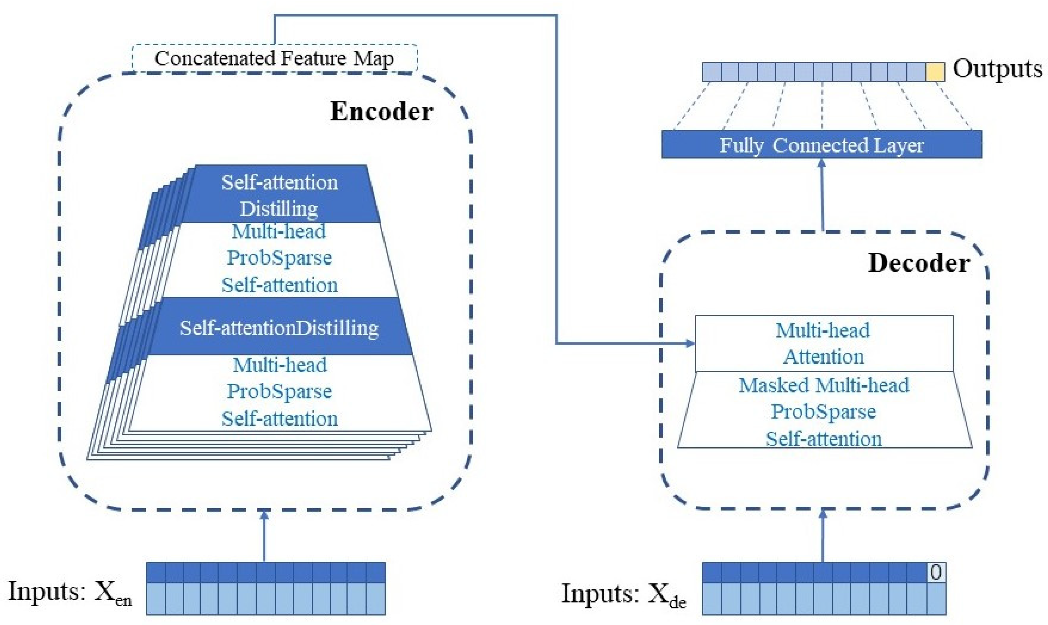
2. Methodology
3. Model Calibration
4. Numerical Example
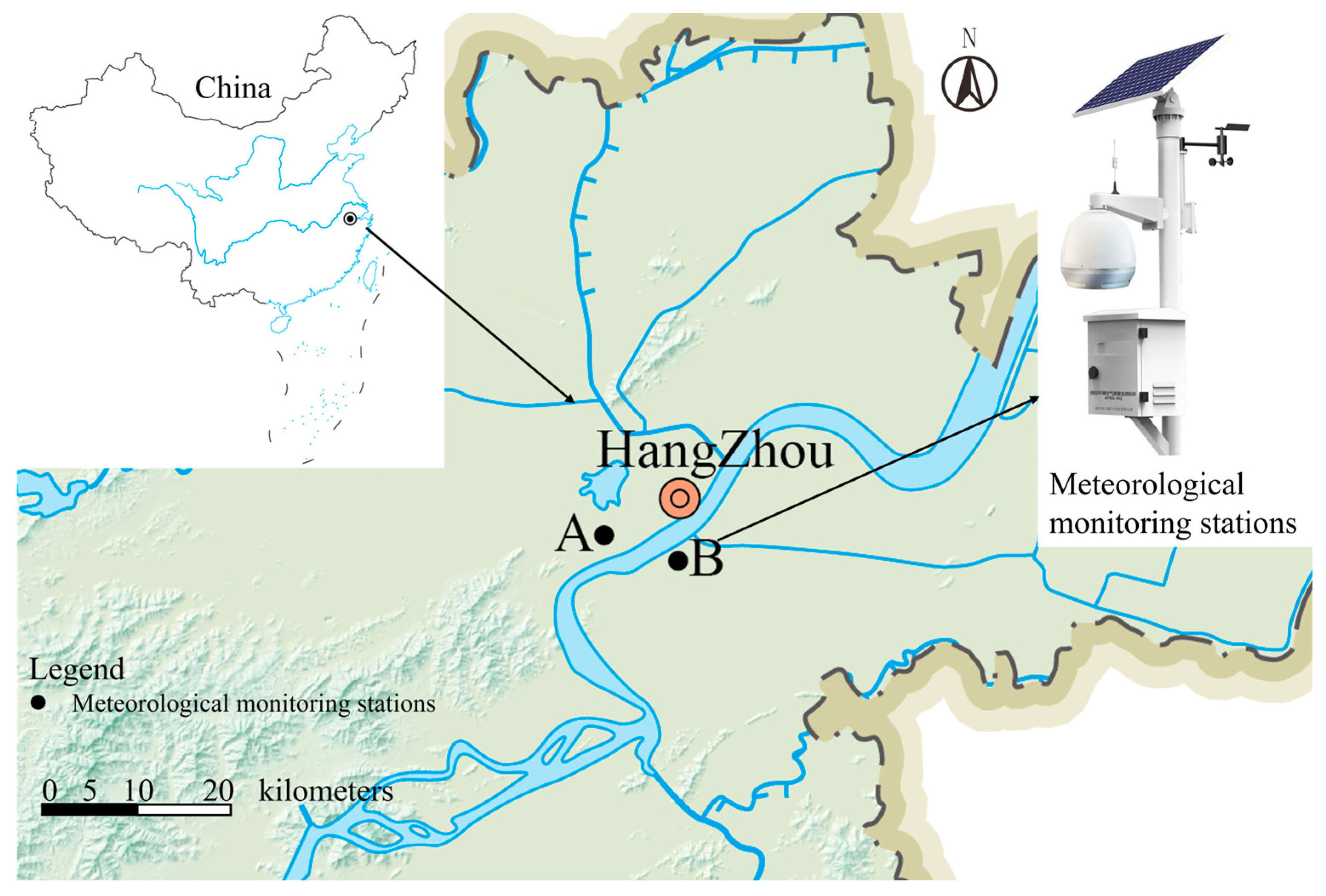
4.1. Study Data
4.1.1. Data
4.1.2. Model Performance Evaluation Metrics
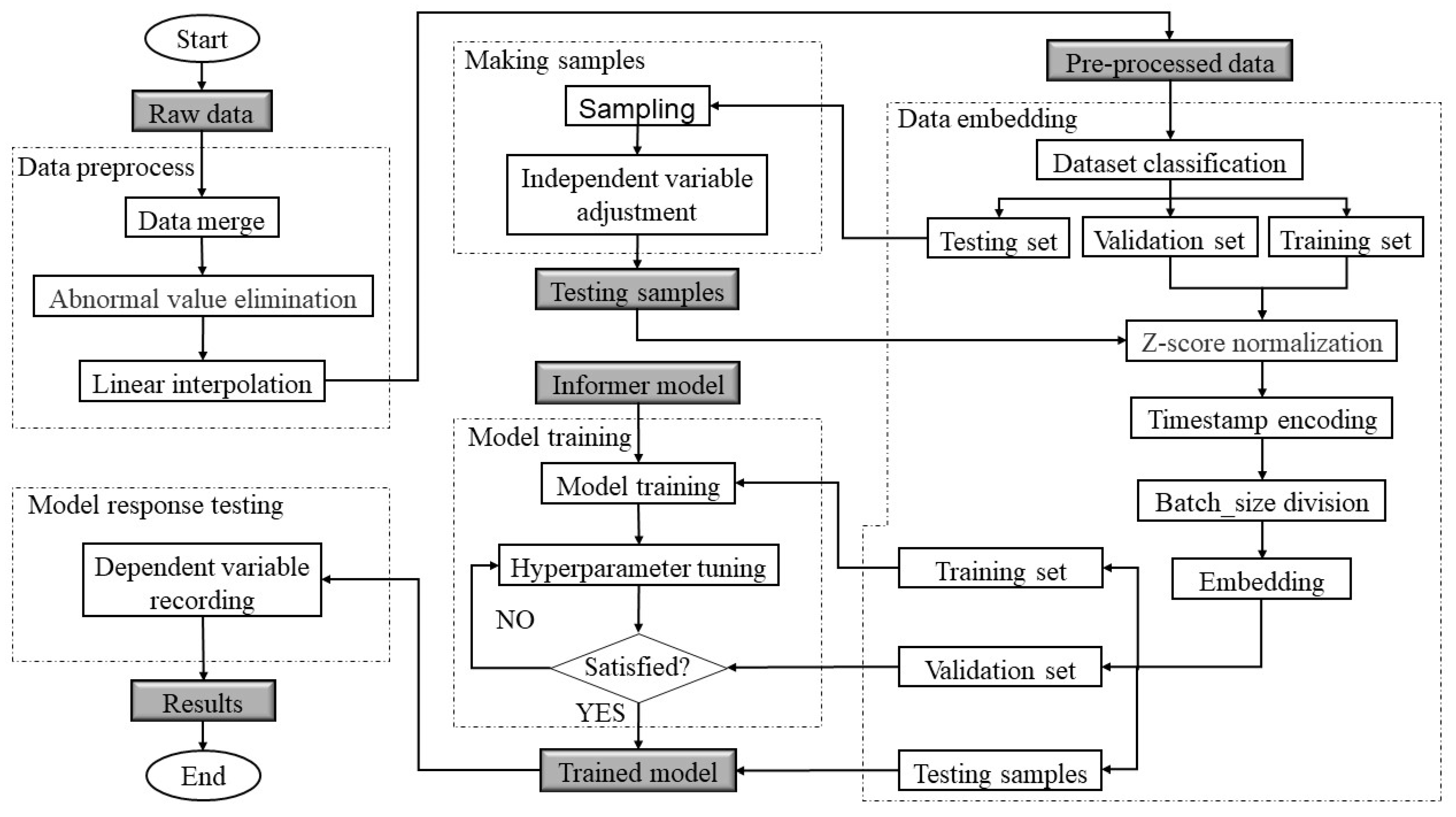
4.2. Research Process
4.2.1. Data Preprocessing
4.2.2. Data Embedding
4.2.3. Model Training
4.2.4. Model Response Testing
4.3. Results
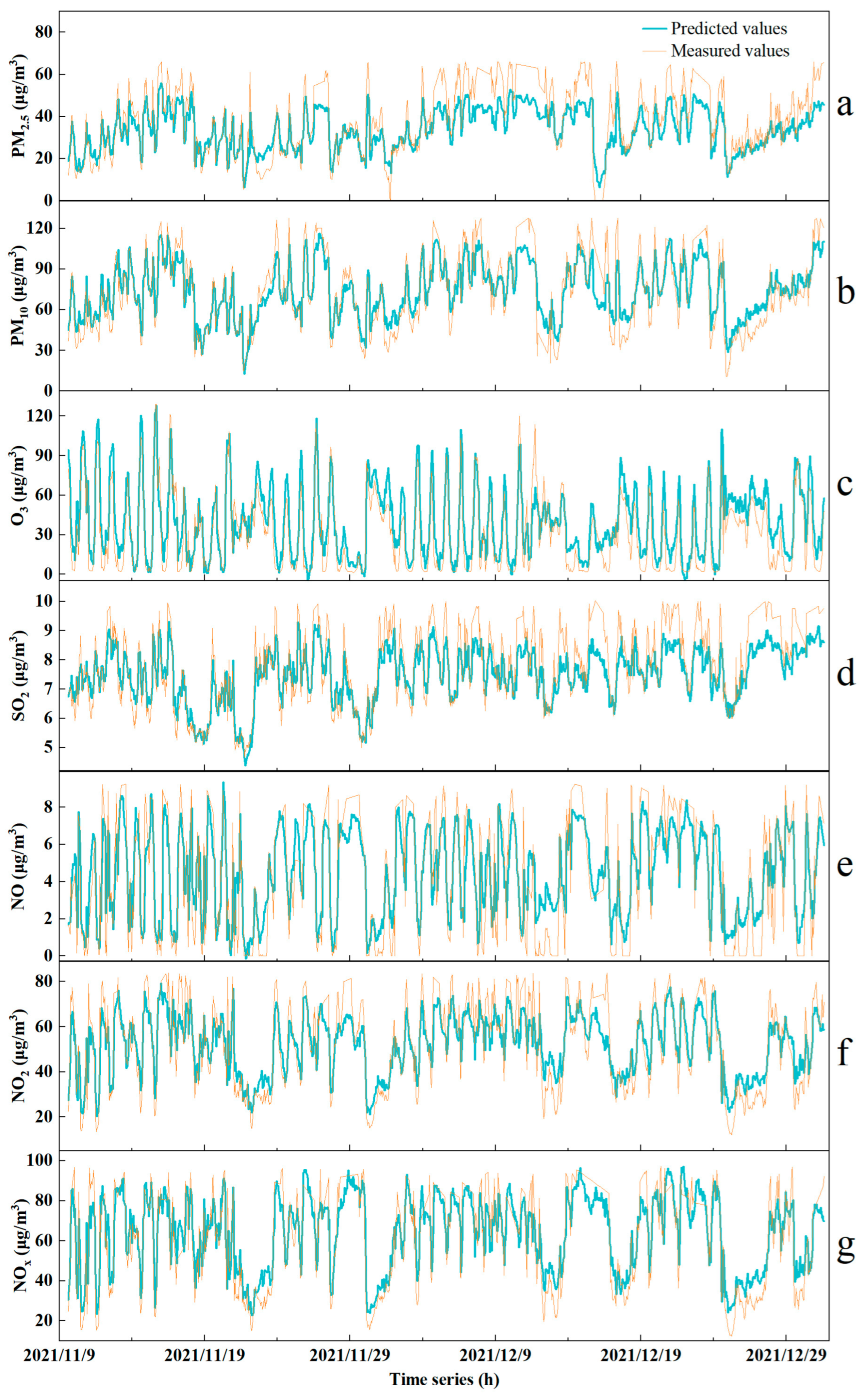
4.3.1. The Predictive Performance of the Model
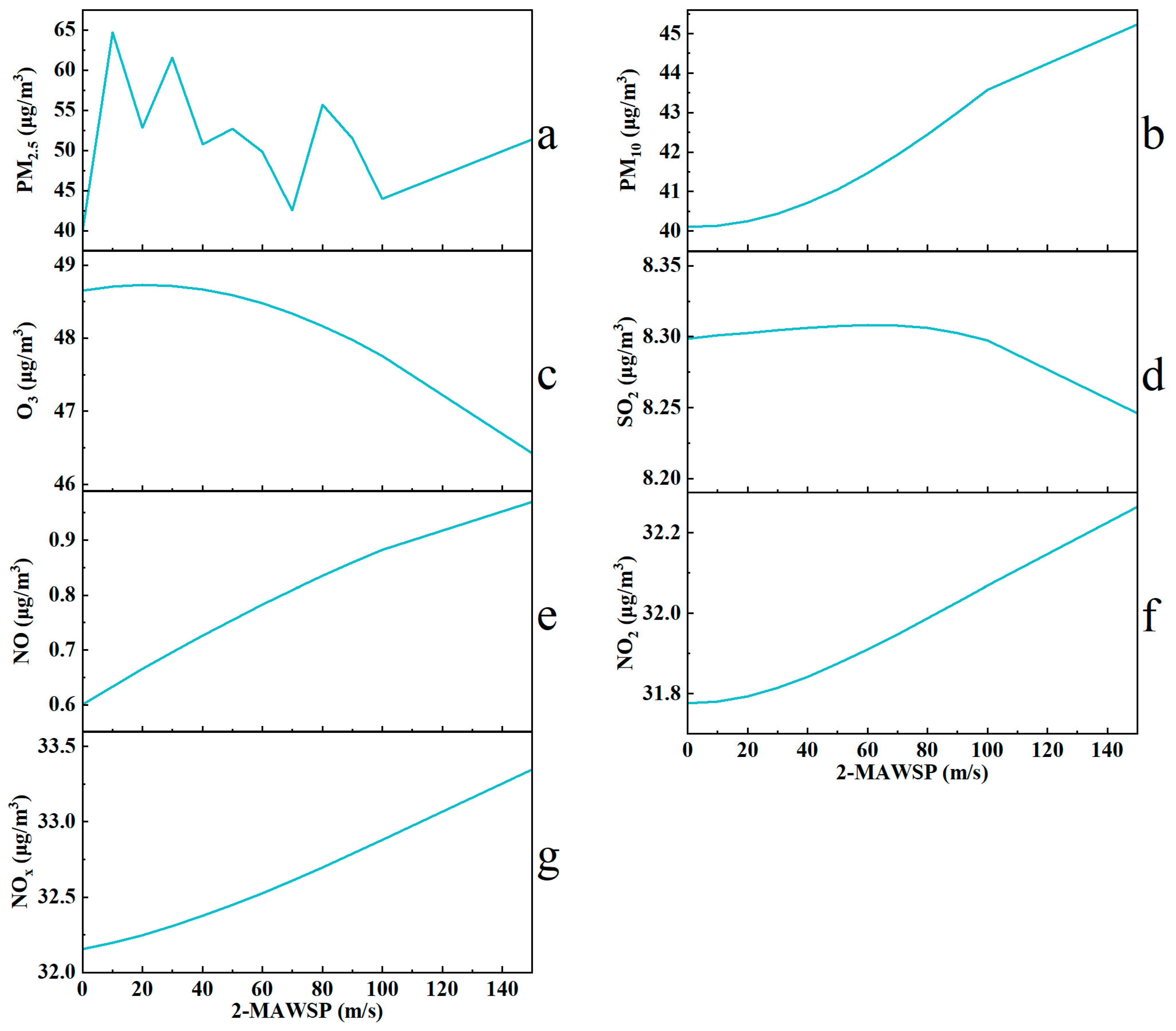
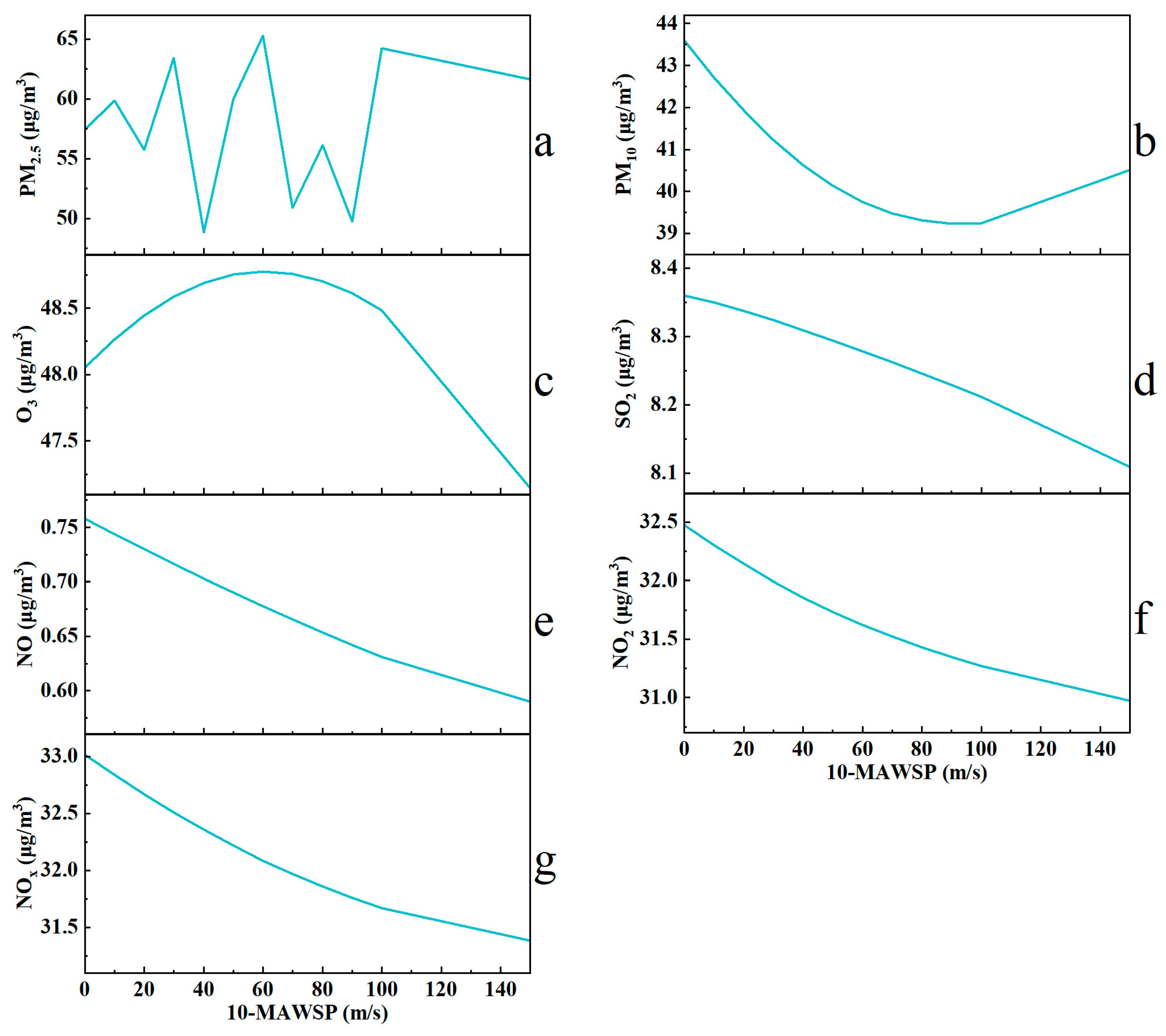
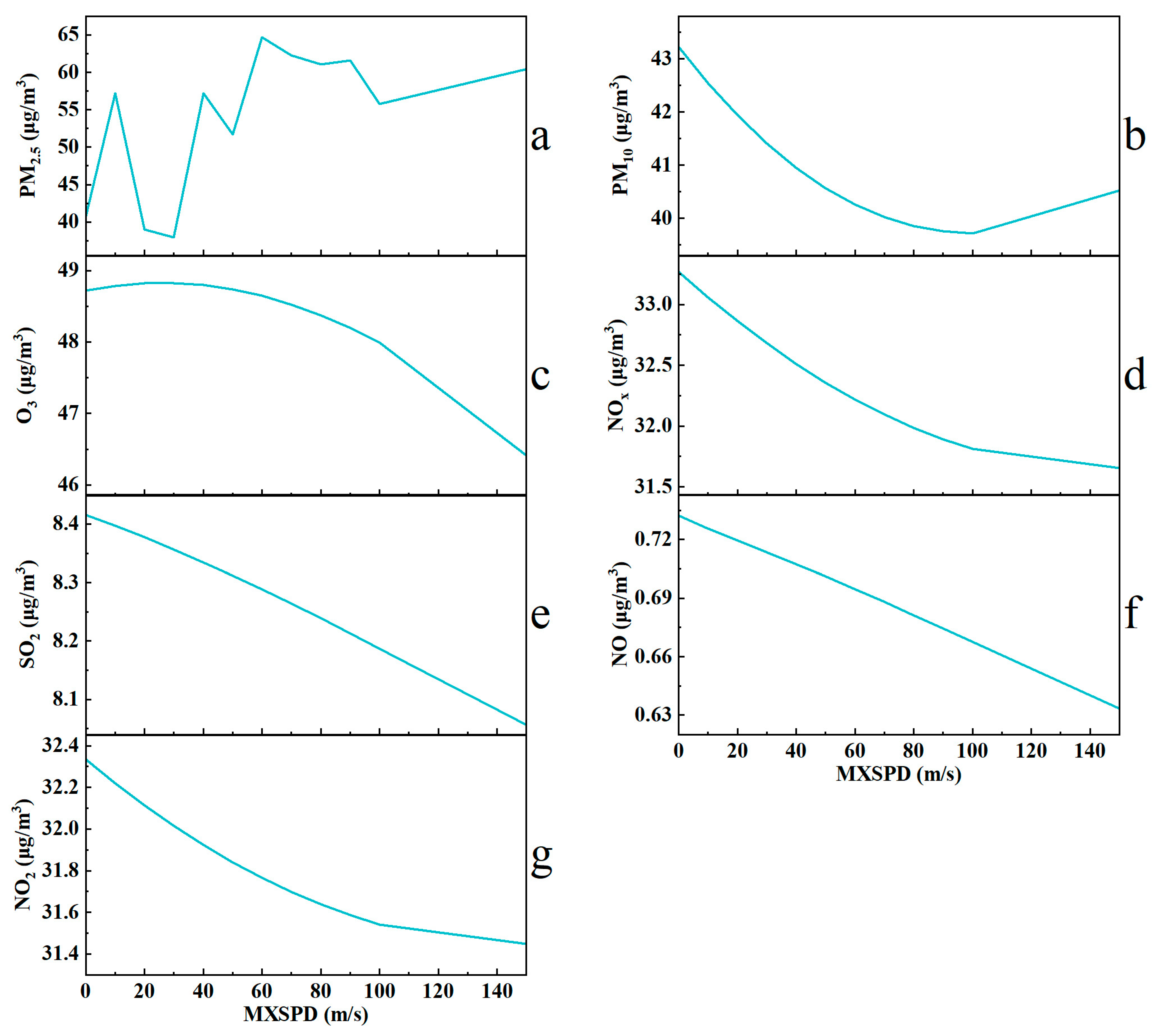
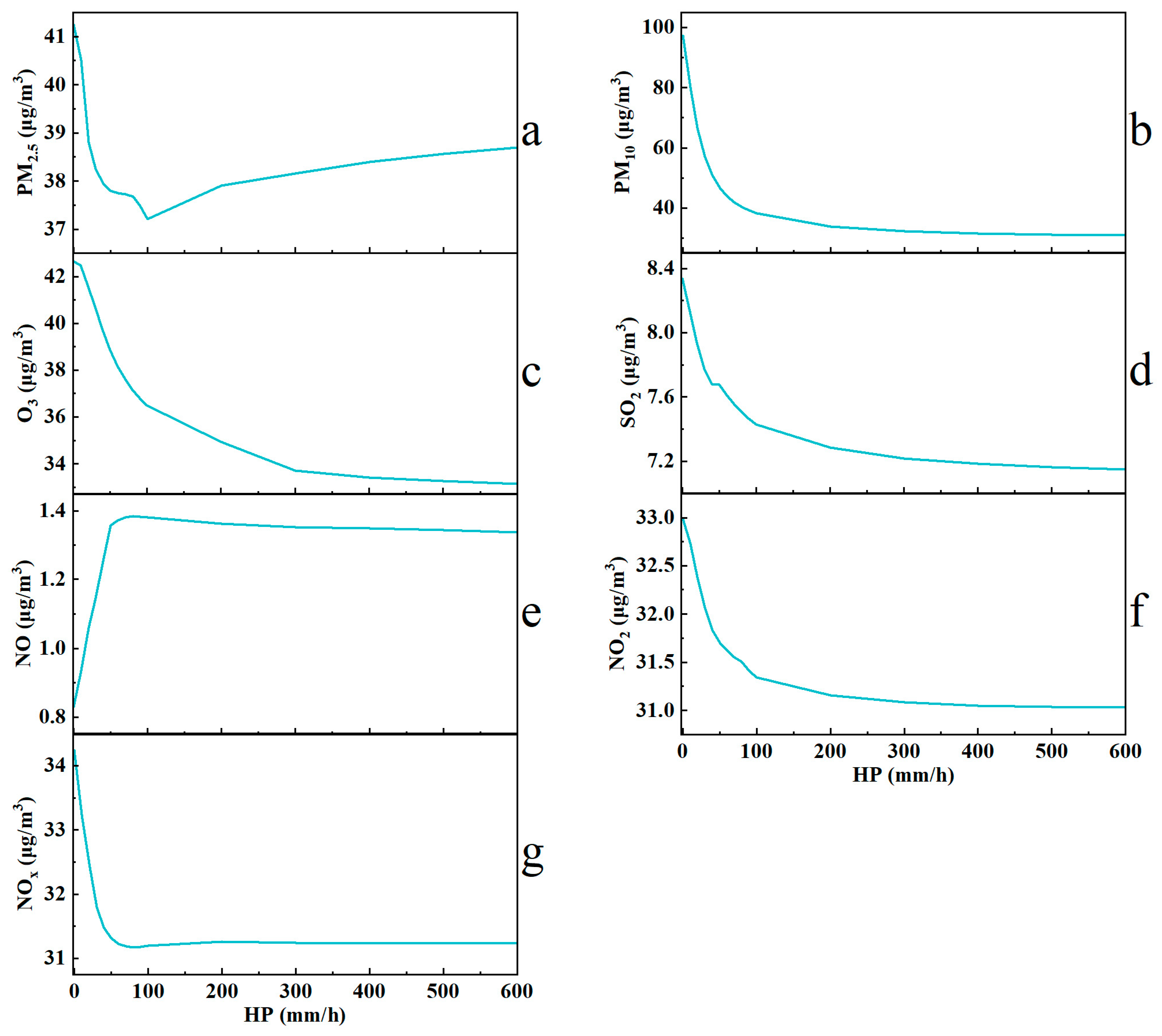
4.3.2. Prediction of Air Quality Parameters’ Response to Different Meteorological Factors
5. Conclusions
- (1)
- The factor of wind has a significant dispersing effect on most air quality parameters. As the wind speed increases, the values of most air quality parameters decrease. For PM10, as the wind speed increases, its concentration shows a tendency to decrease initially and then increase. The primary cause of this phenomenon is that, with a high enough wind speed, dust particles are lifted from the ground, resulting in elevated levels of fine particulate matter concentration in the atmosphere.
- (2)
- HP has an extremely significant reducing effect on almost all air quality parameters. Moreover, the impact of HP has a significant influence on these air quality parameters, making them highly susceptible. During the initial phases of HP enhancement, notable alterations are observed in the measurements of air quality parameters. Afterwards, its transformation is gradual. Except for NO, all other air quality parameter values show varying degrees of decreases.
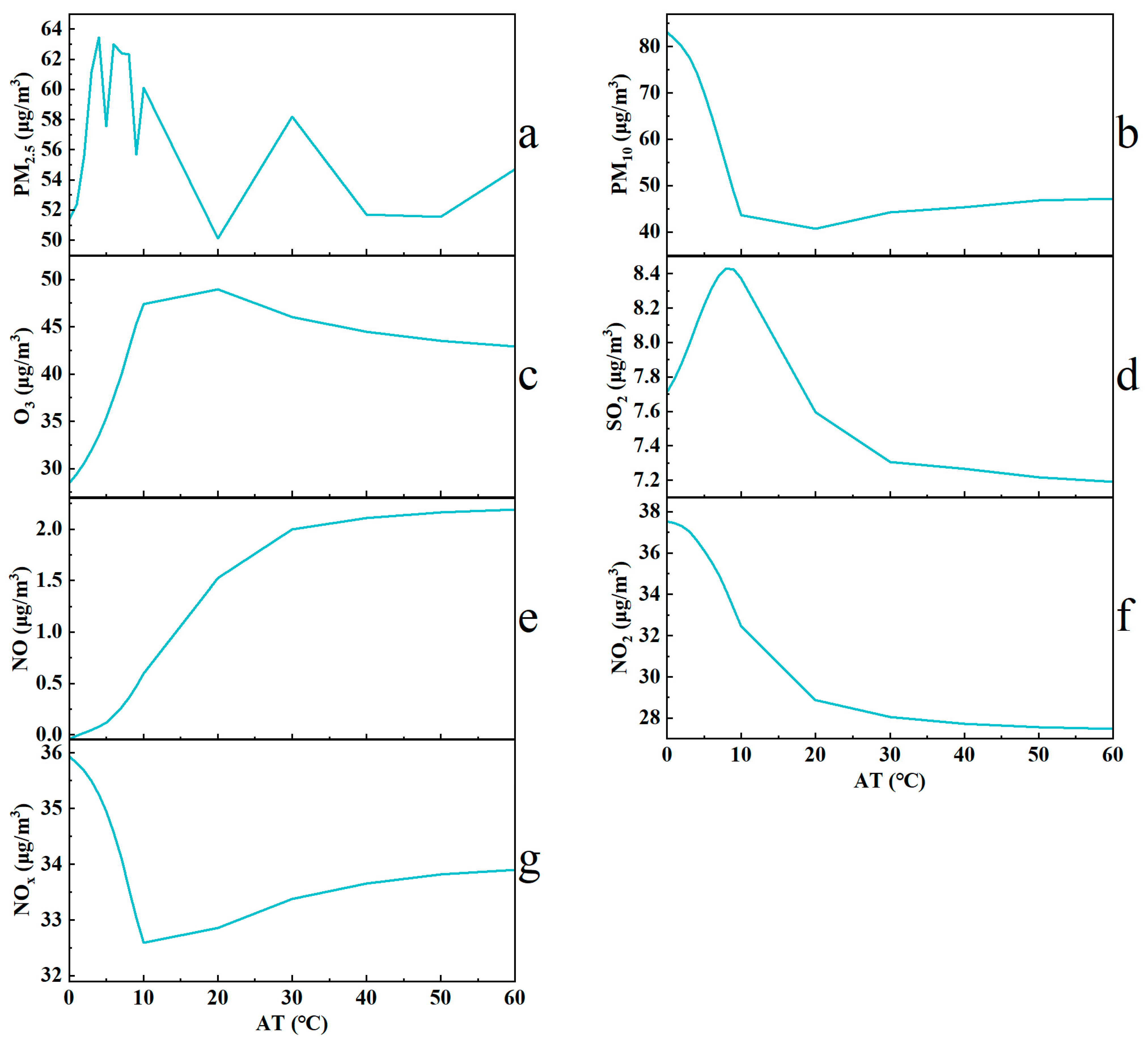
- (3)
- AT has a promoting effect on the increase in O3 and NO concentrations. AT has a decreasing effect on the concentration of PM10 and NO2. For SO2 concentration, AT has a promoting and then inhibiting effect.
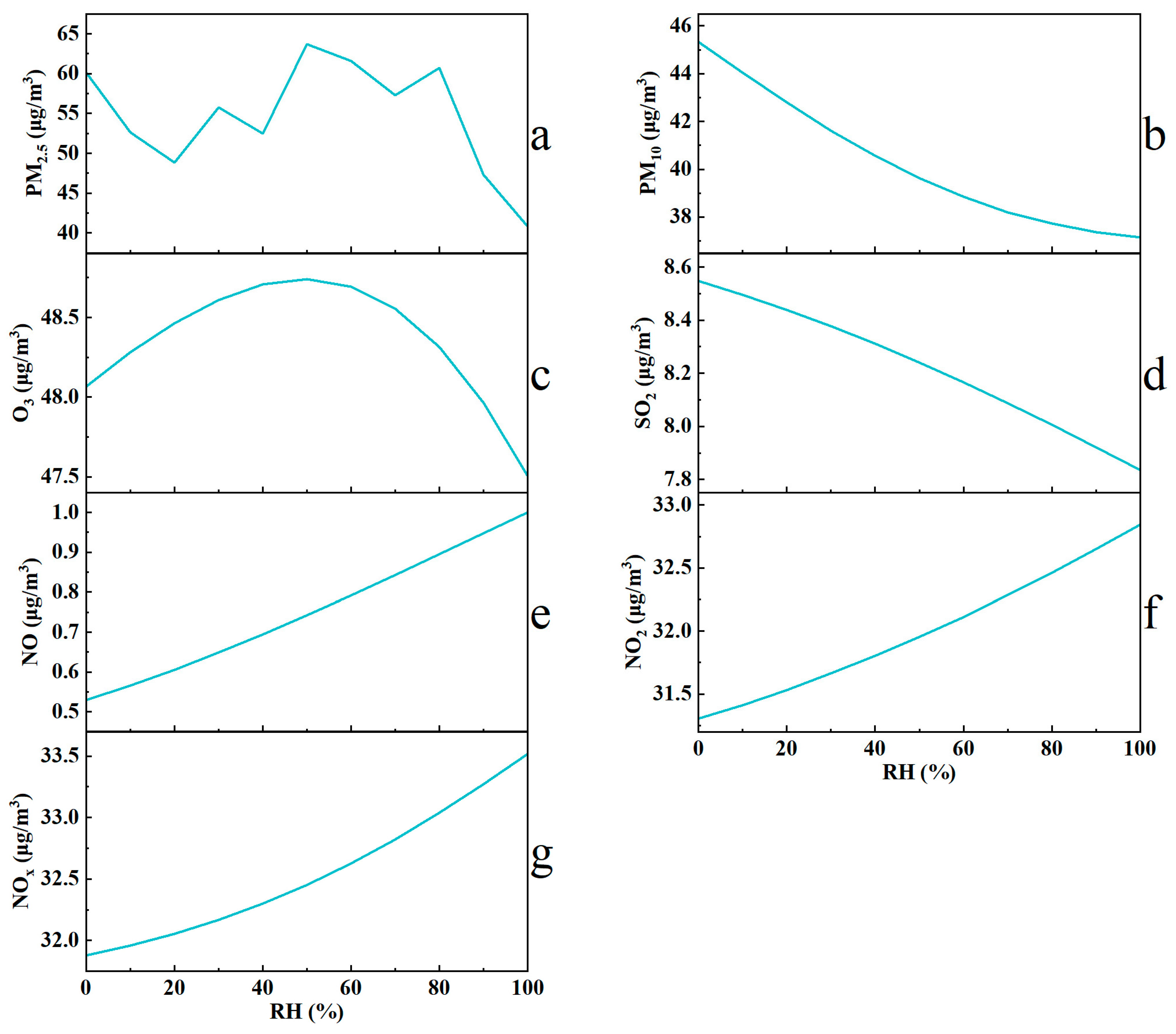
- (4)
- RH has a reducing effect on the concentration of PM10 and SO2, while in contrast, RH has a promoting effect on the concentration of nitrogen oxides. For the concentration of O3, it shows an initial increase followed by a decrease.
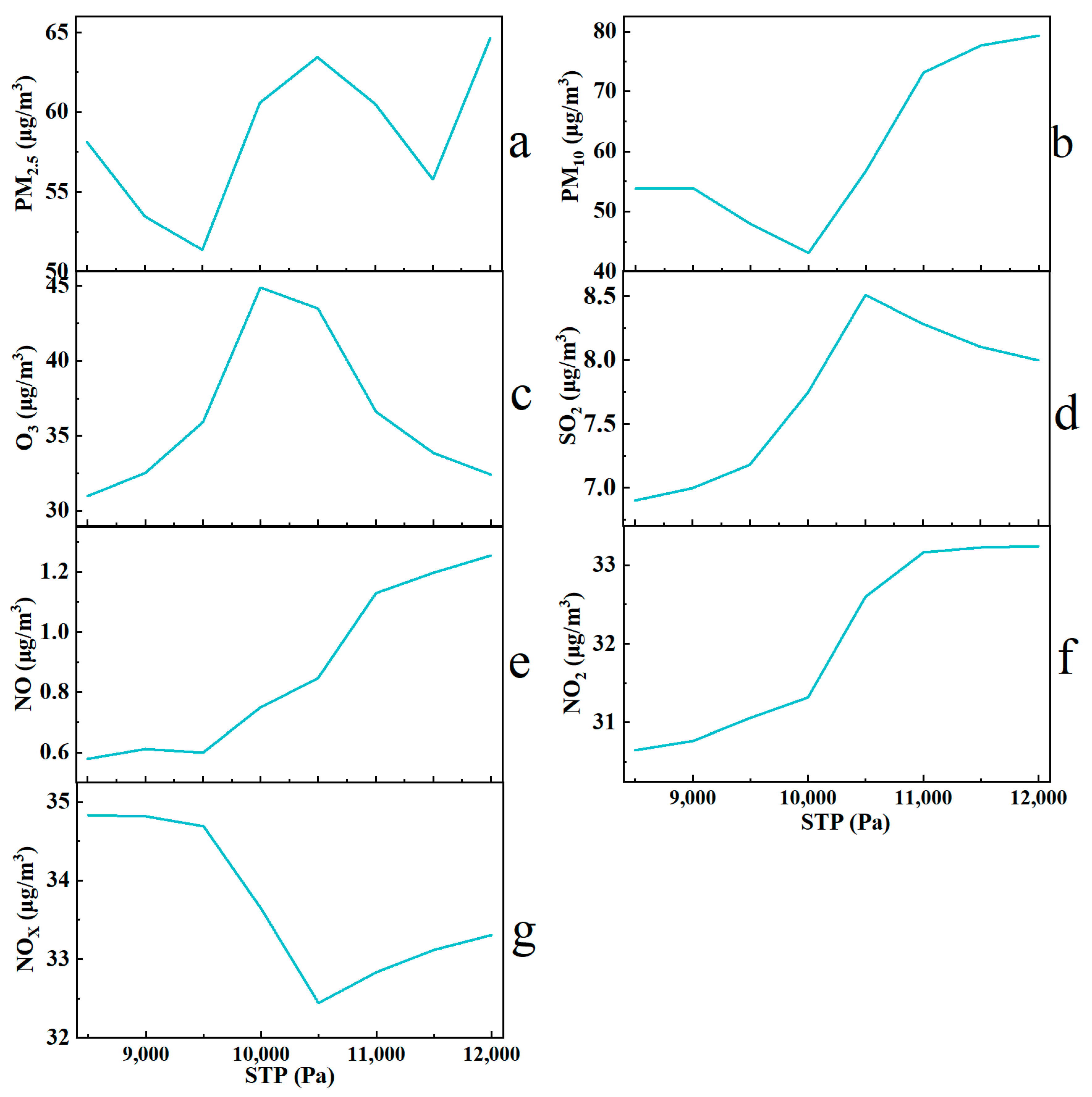
- (5)
- Overall, except for PM2.5, O3, and NOx, STP has a promoting effect on the values of the other air quality parameters. For O3, as STP increases, STP exhibits a promoting and then inhibiting effect on it. On the contrary, for NOx, STP exhibits a first inhibitory and then promoting effect.
Author Contributions
Funding
Institutional Review Board Statement
Informed Consent Statement
Data Availability Statement
Acknowledgments
Conflicts of Interest
Appendix A

| Meteorological Factors | Abbreviations | Unit |
|---|---|---|
| Particulate Matter with an Aerodynamic Diameter Smaller than 2.5 μm | PM2.5 | |
| Particulate Matter with an Aerodynamic Diameter Smaller than 10 μm | PM10 | |
| Sulfur Dioxide | SO2 | |
| Ozone | O3 | |
| Nitric Oxide | NO | |
| Nitrogen Dioxide | NO2 | |
| Nitrogen Oxides | NOx | |
| Carbon Monoxide | CO |
| Meteorological Factors | Abbreviations | Unit |
|---|---|---|
| Maximum Instantaneous Wind Speed | / | |
| Maximum Instantaneous Wind Direction | / | |
| 2-Minute Average Wind Speed | 2-MAWSP | |
| 2-Minute Average Wind Direction | / | |
| 10-Minute Average Wind Speed | 10-MAWSP | |
| 10-Minute Average Wind Direction | / | |
| Extreme Wind Speed | / | |
| Extreme Wind Direction | / | |
| Maximum Wind Speed | MXSPD | |
| Maximum Wind Direction | / | |
| Hourly Precipitation | HP | |
| Air Temperature | AT | |
| Maximum Air Temperature | / | |
| Minimum Air Temperature | / | |
| Relative Humidity | RH | |
| Minimum Relative Humidity | / | |
| Station Pressure | STP | |
| Maximum Air Pressure | / | |
| Minimum Air Pressure | / | |
| Visibility | / | |
| Minimum Visibility | / |
| Abbreviations | |
|---|---|
| Air Pollution Index | API |
| Seasonal-Trend Decomposition Procedure Based on Loess | STL |
| Convergent Cross Mapping | CCM |
| Detrended Fluctuation Analysis | DFA |
| Detrended Cross-Correlation Coefficient Analysis | DCCA |
| ρ Detrended Cross-Correlation Coefficient Analysis | ρDCCA |
| Artificial Intelligence | AI |
| Auto-Regressive Moving Average | ARMA |
| Auto-Regressive Integrated Moving Average | ARIMA |
| Recurrent Neural Networks | RNNs |
| Long Short-Term Memory Network | LSTM |
| Spatiotemporal Transformer | STT |
| Long-Sequence Time Series Forecasting | LSTF |
| ProbSparse Self-Attention | PSSA |
| Self-Attention Distilling | SAD |
| Generative-Style Decoder | GSD |
| Masked Multi-Head ProbSparse Self-Attention | MMHPSSA |
| Multi-Head ProbSparse Self-Attention | MHPSSA |
| Fully Connected Layer | FCL |
| Mean Relative Error | MRE |
| Grey Relation Analysis | GRA |
| Mean Absolute Error | MAE |
| Root Mean Square Error | RMSE |
References
- Ryan, R.G.; Silver, J.D.; Schofield, R. Air quality and health impact of 2019—20 Black Summer megafires and COVID-19 lockdown in Melbourne and Sydney, Australia. Environ. Pollut. 2021, 274, 116498. [Google Scholar] [CrossRef]
- Cobelo, I.; Castelhano, F.J.; Borge, R.; Roig, H.L.; Adams, M.; Amini, H.; Koutrakis, P.; Réquia, W.J. The impact of wildfires on air pollution and health across land use categories in Brazil over a 16-year period. Environ. Res. 2023, 224, 115522. [Google Scholar] [CrossRef] [PubMed]
- Chuvieco, E.; Mouillot, F.; van der Werf, G.R.; San Miguel, J.; Tanase, M.; Koutsias, N.; García, M.; Yebra, M.; Padilla, M.; Gitas, I.; et al. Historical background and current developments for mapping burned area from satellite Earth observation. Remote Sens. Environ. 2019, 225, 45–64. [Google Scholar] [CrossRef]
- Bolaño-Diaz, S.; Camargo-Caicedo, Y.; Bernal, F.T.; Bolaño-Ortiz, T.R. The Effect of Forest Fire Events on Air Quality: A Case Study of Northern Colombia. Fire 2022, 5, 191. [Google Scholar] [CrossRef]
- Li, L.; Qian, J.; Ou, C.-Q.; Zhou, Y.-X.; Guo, C.; Guo, Y. Spatial and temporal analysis of Air Pollution Index and its timescale-dependent relationship with meteorological factors in Guangzhou, China, 2001–2011. Environ. Pollut. 2014, 190, 75–81. [Google Scholar] [CrossRef]
- Chen, Z.; Cai, J.; Gao, B.; Xu, B.; Dai, S.; He, B.; Xie, X. Detecting the causality influence of individual meteorological factors on local PM 2.5 concentration in the Jing-Jin-Ji region. Sci. Rep. 2017, 7, 40735. [Google Scholar]
- Palmeira, A.; Pereira, É.; Ferreira, P.; Diele-Viegas, L.M.; Moreira, D.M. Long-Term Correlations and Cross-Correlations in Meteorological Variables and Air Pollution in a Coastal Urban Region. Sustainability 2022, 14, 14470. [Google Scholar] [CrossRef]
- Hu, M.; Wang, Y.; Wang, S.; Jiao, M.; Huang, G.; Xia, B. Spatial-temporal heterogeneity of air pollution and its relationship with meteorological factors in the Pearl River Delta, China. Atmos. Environ. 2021, 254, 118415. [Google Scholar] [CrossRef]
- Li, X.; Song, H.; Zhai, S.; Lu, S.; Kong, Y.; Xia, H.; Zhao, H. Particulate matter pollution in Chinese cities: Areal-temporal variations and their relationships with meteorological conditions (2015–2017). Environ. Pollut. 2019, 246, 11–18. [Google Scholar] [CrossRef]
- Kim, M.H.; Kim, Y.S.; Lim, J.; Kim, J.T.; Sung, S.W.; Yoo, C. Data-driven prediction model of indoor air quality in an underground space. Korean J. Chem. Eng. 2010, 27, 1675–1680. [Google Scholar] [CrossRef]
- Li, X.; Peng, L.; Hu, Y.; Shao, J.; Chi, T. Deep learning architecture for air quality predictions. Environ. Sci. Pollut. Res. 2016, 23, 22408–22417. [Google Scholar] [CrossRef] [PubMed]
- Liu, H.; Li, Q.; Yu, D.; Gu, Y. Air Quality Index and Air Pollutant Concentration Prediction Based on Machine Learning Algorithms. Appl. Sci. 2019, 9, 4069. [Google Scholar] [CrossRef]
- Navares, R.; Aznarte, J.L. Predicting air quality with deep learning LSTM: Towards comprehensive models. Ecol. Inform. 2020, 55, 101019. [Google Scholar] [CrossRef]
- Seng, D.; Zhang, Q.; Zhang, X.; Chen, G.; Chen, X. Spatiotemporal prediction of air quality based on LSTM neural network. Alex. Eng. J. 2021, 60, 2021–2032. [Google Scholar] [CrossRef]
- Das, B.; Dursun, O.O.; Toraman, S. Prediction of air pollutants for air quality using deep learning methods in a metropolitan city. Urban Clim. 2022, 46, 101291. [Google Scholar] [CrossRef]
- Wang, K.; Liu, B.; Yang, X.; Fan, X.; Zhou, Z. Spatial and temporal evolution characteristics of air quality based on EWM-LSTM model: A case study of Sichuan Province, China. Air Qual. Atmos. Health 2023, 13, 10152. [Google Scholar] [CrossRef]
- Ratkovic, K.; Kovac, N.; Simeunovic, M. Hybrid LSTM Model to Predict the Level of Air Pollution in Montenegro. Appl. Sci. 2023, 13, 10152. [Google Scholar] [CrossRef]
- Zheng, G.; Liu, H.; Yu, C.; Li, Y.; Cao, Z. A new PM2.5 forecasting model based on data preprocessing, reinforcement learning and gated recurrent unit network. Atmos. Pollut. Res. 2022, 13, 101475. [Google Scholar] [CrossRef]
- Yang, J.; Zhou, X. Prediction of PM2.5 concentration based on ARMA model based on wavelet transform. In Proceedings of the 2020 12th International Conference on Intelligent Human-Machine Systems and Cybernetics (IHMSC), Hangzhou, China, 22–23 August 2020; IEEE: New York, NY, USA, 2020. [Google Scholar]
- Wang, P.; Zhang, H.; Qin, Z.; Zhang, G. A novel hybrid-Garch model based on ARIMA and SVM for PM 2.5 concentrations forecasting. Atmos. Pollut. Res. 2017, 8, 850–860. [Google Scholar] [CrossRef]
- Zhang, L.; Lin, J.; Qiu, R.; Hu, X.; Zhang, H.; Chen, Q.; Tan, H.; Lin, D.; Wang, J. Trend analysis and forecast of PM2.5 in Fuzhou, China using the ARIMA model. Ecol. Indic. 2018, 95, 702–710. [Google Scholar] [CrossRef]
- Tsai, Y.; Zeng, Y.; Chang, Y. Air pollution forecasting using RNN with LSTM. In Proceedings of the 2018 IEEE 16th Intl Conf on Dependable, Autonomic and Secure Computing, 16th Intl Conf on Pervasive Intelligence and Computing, 4th Intl Conf on Big Data Intelligence and Computing and Cyber Science and Technology Congress (DASC/PiCom/DataCom/CyberSciTech), Athens, Greece, 12–15 August 2018; IEEE: New York, NY, USA, 2018. [Google Scholar]
- Kristiani, E.; Lin, H.; Lin, J.R.; Chuang, Y.H.; Huang, C.Y.; Yang, C.T. Short-Term Prediction of PM 2.5 Using LSTM Deep Learning Methods. Sustainability 2022, 14, 2068. [Google Scholar] [CrossRef]
- Du, S.; Li, T.; Yang, Y.; Horng, S.J. Deep air quality forecasting using hybrid deep learning framework. IEEE Trans. Knowl. Data Eng. 2019, 33, 2412–2424. [Google Scholar] [CrossRef]
- Zhu, J.; Deng, F.; Zhao, J.; Zheng, H. Attention-based parallel networks (APNet) for PM2.5 spatiotemporal prediction. Sci. Total Environ. 2021, 769, 145082. [Google Scholar] [CrossRef] [PubMed]
- Vaswani, A.; Shazeer, N.; Parmar, N.; Uszkoreit, J.; Jones, L.; Gomez, A.N.; Kaiser, Ł.; Polosukhin, I. Attention is all you need. Adv. Neural Inf. Process. Syst. 2017, 30, 6000–6010. [Google Scholar]
- Yu, M.; Masrur, A.; Blaszczak-Boxe, C. Predicting hourly PM 2.5 concentrations in wildfire-prone areas using a SpatioTemporal Transformer model. Sci. Total Environ. 2023, 860, 160446. [Google Scholar] [CrossRef] [PubMed]
- Zhou, H.; Zhang, S.; Peng, J.; Zhang, S.; Li, J.; Xiong, H.; Zhang, W. Informer: Beyond efficient transformer for long sequence time-series forecasting. In Proceedings of the AAAI Conference on Artificial Intelligence, Virtual, 29 February 2021. [Google Scholar]
- Gong, M.; Zhao, Y.; Sun, J.; Han, C.; Sun, G.; Yan, B. Load forecasting of district heating system based on Informer. Energy 2022, 253, 124179. [Google Scholar] [CrossRef]
- Lai, K.; Xu, H.; Sheng, J.; Huang, Y. Hour-by-Hour Prediction Model of Air Pollutant Concentration Based on EIDW-Informer-A Case Study of Taiyuan. Atmosphere 2023, 14, 1274. [Google Scholar] [CrossRef]
- Guo, L.-C.; Zhang, Y.; Lin, H.; Zeng, W.; Liu, T.; Xiao, J.; Rutherford, S.; You, J.; Ma, W. The washout effects of rainfall on atmospheric particulate pollution in two Chinese cities. Environ. Pollut. 2016, 215, 195–202. [Google Scholar] [CrossRef]
- Zhang, H.; Wang, Y.; Hu, J.; Ying, Q.; Hu, X.-M. Relationships between meteorological parameters and criteria air pollutants in three megacities in China. Environ. Res. 2015, 140, 242–254. [Google Scholar] [CrossRef] [PubMed]
- He, J.; Gong, S.; Yu, Y.; Yu, L.; Wu, L.; Mao, H.; Song, C.; Zhao, S.; Liu, H.; Li, X.; et al. Air pollution characteristics and their relation to meteorological conditions during 2014–2015 in major Chinese cities. Environ. Pollut. 2017, 223, 484–496. [Google Scholar] [CrossRef]
- Wang, D.; Hu, H.; Chen, D. Transformer with sparse self-attention mechanism for image captioning. Electron. Lett. 2020, 56, 764–766. [Google Scholar] [CrossRef]
- Li, T.; Jin, W.; Fu, R.; He, C. Daytime sea fog monitoring using multimodal self-supervised learning with band attention mechanism. Neural Comput. Appl. 2022, 34, 21205–21222. [Google Scholar] [CrossRef]
- Fei, X.; Ling, Q. Attention-based global and local spatial-temporal graph convolutional network for vehicle emission prediction. Neurocomputing 2023, 521, 41–55. [Google Scholar] [CrossRef]
- Wang, K.; Li, K.; Zhou, L.; Hu, Y.; Cheng, Z.; Liu, J.; Chen, C. Multiple convolutional neural networks for multivariate time series prediction. Neurocomputing 2019, 360, 107–119. [Google Scholar] [CrossRef]
- Cleophas, T.J.; Zwinderman, A.H.; Cleophas, T.J.; Zwinderman, A.H. Bayesian Pearson correlation analysis. In Modern Bayesian Statistics in Clinical Research; Springer: Berlin/Heidelberg, Germany, 2018; pp. 111–118. [Google Scholar]
- Fu, B.; Gao, X.H.; Wu, L. Grey relational analysis for the AQI of Beijing, Tianjin, and Shijiazhuang and related countermeasures. Grey Syst.-Theory Appl. 2018, 8, 156–166. [Google Scholar] [CrossRef]
- Zhou, J.; Wang, Y.; Xiao, F.; Wang, Y.; Sun, L. Water Quality Prediction Method Based on IGRA and LSTM. Water 2018, 10, 1148. [Google Scholar] [CrossRef]


| Hyperparameters | Value | Hyperparameters | Value |
|---|---|---|---|
| Time encoding length | Hour | Number of heads of attention | 8 |
| Encoder step size | 12 | Encoder stacking | 3, 2, 1 |
| Decoder step size | 12 | Regularization settings | 0.05 |
| Prediction step size | 1 | Activation function | gelu |
| Encoding dimension | 29 | batch size | 32 |
| Decoding dimensions | 29 | Initial learning rate | 0.0001 |
| Output dimensions | 1 | loss function | mse |
| Time Step | Maximum Instantaneous Wind Speed | … | HP | … | PM2.5 |
|---|---|---|---|---|---|
| 1 | 20 | 0 | 40.67 | ||
| 2 | 16 | 2 | 35.25 | ||
| ⋮ | … | … | ⋮ | … | ⋮ |
| 12 | 43 | 0 | 48.02 | ||
| 13 | 60 | 0 | 43.5 |
| Pollutants Predicted by the Model | MAE | RMSE |
|---|---|---|
| PM2.5 | 7.70% | 9.46% |
| PM10 | 10.32% | 12.99% |
| O3 | 13.76% | 16.50% |
| SO2 | 0.95% | 1.16% |
| NO | 2.20% | 2.67% |
| NO2 | 7.16% | 9.06% |
| NOx | 8.50% | 10.55% |
Disclaimer/Publisher’s Note: The statements, opinions and data contained in all publications are solely those of the individual author(s) and contributor(s) and not of MDPI and/or the editor(s). MDPI and/or the editor(s) disclaim responsibility for any injury to people or property resulting from any ideas, methods, instructions or products referred to in the content. |
© 2024 by the authors. Licensee MDPI, Basel, Switzerland. This article is an open access article distributed under the terms and conditions of the Creative Commons Attribution (CC BY) license (https://creativecommons.org/licenses/by/4.0/).
Share and Cite
Tian, X.; Zhang, C.; Liu, H.; Zhang, B.; Lu, C.; Jiao, P.; Ren, S. Research on Air Quality in Response to Meteorological Factors Based on the Informer Model. Sustainability 2024, 16, 6794. https://doi.org/10.3390/su16166794
Tian X, Zhang C, Liu H, Zhang B, Lu C, Jiao P, Ren S. Research on Air Quality in Response to Meteorological Factors Based on the Informer Model. Sustainability. 2024; 16(16):6794. https://doi.org/10.3390/su16166794
Chicago/Turabian StyleTian, Xiaoqing, Chaoqun Zhang, Huan Liu, Baofeng Zhang, Cheng Lu, Pengfei Jiao, and Songkai Ren. 2024. "Research on Air Quality in Response to Meteorological Factors Based on the Informer Model" Sustainability 16, no. 16: 6794. https://doi.org/10.3390/su16166794
APA StyleTian, X., Zhang, C., Liu, H., Zhang, B., Lu, C., Jiao, P., & Ren, S. (2024). Research on Air Quality in Response to Meteorological Factors Based on the Informer Model. Sustainability, 16(16), 6794. https://doi.org/10.3390/su16166794