Article

ARIMA-Driven Vegetable Pricing and Restocking Strategy for Dual Optimization of Freshness and Profitability in Supermarket Perishables

1
School of Transportation and Civil Engineering, Nantong University, Nantong 226019, China
2
School of Mechanical Engineering, Nantong University, Nantong 226019, China
*
Authors to whom correspondence should be addressed.
Sustainability 2024, 16(10), 4071; https://doi.org/10.3390/su16104071
Submission received: 9 March 2024 / Revised: 5 May 2024 / Accepted: 9 May 2024 / Published: 13 May 2024

Abstract

:
In the evolving landscape of perishable goods management, where the balance between minimizing waste and maximizing profitability is paramount, this work introduces an innovative approach to pricing and inventory decisions for products with limited shelf lives, focusing on vegetables in supermarkets. The contribution lies in its integration of an automated pricing and restocking decision model that leverages autoregressive integrated moving average (ARIMA) forecasting techniques alongside dynamic pricing strategies tailored to the goods’ freshness and remaining shelf life. The study uses a comprehensive sales, spoilage rates, and customer demand dataset to apply ARIMA forecasting for optimal restocking and adjusts prices dynamically based on product freshness, promoting competitive pricing and waste reduction. The results demonstrate the model’s effectiveness, reducing spoilage rates by up to 30% and increasing profitability margins by about 15%, highlighting its practical utility in real-world scenarios. The research highlights the potential for supermarkets to improve perishable goods inventory management, leading to significant economic benefits and reduced food waste. This study contributes to sustainable retail practices aligning with global responsible consumption and production initiatives, offering a scalable economic efficiency and environmental stewardship solution.

1. Introduction

Perishable products like fruits, vegetables, seafood, and meats have become essential daily, significantly impacting the global economy. These products, short-shelf-life or seasonal produce, made up 59.1% of U.S. supermarket sales. In 2022, China’s food and grocery retail market reached USD 77.3 trillion, while the U.K.’s was valued at about GBP 193.6 billion in 2019. However, damage and spoilage make fresh produce costly for retailers. Fresh produce spoilage rates in Europe can reach 15%, leading to billions of dollars in annual losses [1]. The U.S. fresh food retail industry annually incurs about USD 30 billion in losses [2]. In China, over 25% of fresh produce was damaged in transportation and retailing in 2015 [3,4], leading to nearly 200 million tons of annual loss, causing significant resource waste and economic losses for farmers. Therefore, effective fresh produce management is crucial for retailers.
Over time, produce on shelves loses freshness, becoming less appealing to quality-conscious consumers [5]. Retailers must continuously introduce new products to maintain a competitive advantage and profit from pricing strategies, like setting higher prices for fresh batches [6,7]. Thus, fresh products should be replenished before the old batches sell out. The cycles of old and new products overlap, coexisting for extended periods [8]. Inventory optimization for perishable goods is complex due to the direct impact of freshness on consumer demand. Nahmias first reviewed deteriorating goods inventory models [9], which Goyala and Giri later extended [10]. Between 2011 and 2016, fresh or perishable goods emerged as an independent research category. Detailed overviews are available in [11,12].
The fresh produce market is rapidly growing and shows great potential, yet its preservation methods need urgent improvement. Consumers in this market are price-sensitive, with prices directly impacting their purchasing decisions. Over time, as product freshness decreases, failure to reduce prices can diminish consumer interest and lead to product stagnation. Therefore, retailers should reduce prices promptly when freshness decreases to stimulate sales. In the supermarket sales model for fresh food, vegetables have a short shelf life. Supermarkets often use automatic pricing and replenishment to maximize revenue and minimize waste based on historical sales and market demand. For vegetables, the cost-plus pricing method is used. The most reasonable prices are derived from analyzing historical costs, unit sales prices, and the supply–demand relationship. Simultaneously, a replenishment forecasting model, combining historical sales and demand data, is built to align replenishment with sales, meeting market demand. Damaged or deteriorated commodities are typically sold at a discount. This paper focuses on establishing an automatic pricing and replenishment model for vegetables to maximize superstore benefits. Figure 1 depicts the process for addressing the vegetable sales issue.
The ARIMA model, devised in the 1970s by American statistician Jenkins and British statistician Box, serves primarily for short-term forecasting of time series variables. Although individual time series values are inherently unpredictable, the model discerns underlying regularities within the overall time series, expressing them mathematically to facilitate short-term predictions.
In the evolving field of perishable goods management, it is essential to balance waste reduction with profit maximization. This study explores the complex dynamics of vegetable sales in supermarkets, analyzing extensive data from 1 July 2020 to 30 June 2023, which include detailed information on sales, loss rates, and customer demand for six primary vegetable categories. The analysis thoroughly examines the distribution patterns and correlations of sales volumes within each category and for individual products. The study integrates Autoregressive Integrated Moving Average (ARIMA) forecasting techniques with dynamic pricing strategies, which are tailored based on product freshness and remaining shelf life. This integration facilitates the development of automated models for pricing and inventory replenishment. By analyzing historical consumer purchasing behavior, the study uncovers insights into the relationships between different categories and examines the differences and correlations among category variables. These findings offer practical guidance for supermarket restocking practices. Additionally, the study performs regression analyses on the total sales volume and unit price for each category, aiding in the formulation of effective restocking and pricing strategies. Beyond focusing on inventory requirements, the research includes a reverse analysis of anticipated sales volumes and employs linear hypotheses to segment the sales cycle into distinct phases. This segmentation allows for systematic modeling of inventory changes and devising optimal replenishment plans.

2. Literature Review

2.1. Replenishment Strategy

Existing research on vegetable inventory restocking strategies falls into two main categories: traditional inventory management theories, like the EOQ and safety stock models, focusing on vegetable characteristics like seasonality and harvesting maturity, and models for perishable inventory that examine restocking strategies. Chen et al. [13] explored dynamic pricing and inventory decisions in perishable product supply chains, considering factors like retailer quality requirements, cost, transportation time, and capacity. Ping et al. [14] enhanced supermarket profitability by optimizing vegetable restocking and pricing strategies through advanced data analytics, uncovering sales patterns and forecasting demand to address the challenges of short shelf lives and varying quality. Chen et al. [15] investigated optimal restocking strategies for farming products in uncertain demand. Using Stackelberg game theory, Huang et al. [16] examined inventory and pricing decisions in a dual-channel supply chain with stochastic demand. He et al. [17] analyzed inventory and pricing strategies in both centralized and decentralized scenarios, coordinating through profit-sharing and tariff contracts. Shen and Li [18] constructed a supply chain inventory model for farmer cooperatives + distribution centers + supermarkets, factoring in the influence of freshness and sale price on demand, and resolved the non-linear optimization problem with an improved genetic algorithm. These studies offer various models for vegetable product inventory management, focusing on demand forecasting and inventory levels based on the principle of supply–demand balance, effectively predicting demand and managing inventory.
Several studies have concentrated on inventory restocking strategies for various vegetable types. Wang and Liu [19] investigated dynamic pricing and inventory control for fresh agricultural products in online retail, focusing on how forward buying behavior affects retailer profits. Sabir [20] studied the perishability, seasonal demand, shelf life, and price elasticity of perishable products, focusing on how retailers can devise demand forecasting, inventory control, and ordering strategies for seasonal fruits and vegetables to minimize losses and maximize profits. Eero [21] explored retailer strategies for managing seasonal fruits and vegetables variability, quality, and demand to ensure adequate stocking and meet customer expectations. In summary, although traditional inventory management theories offer theoretical support for vegetable restocking strategies, the unique and perishable nature of these products makes their inventory management exceptionally challenging. There is a continuous need to explore innovative technologies and methods to advance research, thereby improving the efficiency and accuracy of inventory management.

2.2. Dynamic Pricing

Dynamic pricing, originating from dynamic programming and a foundational model in operations research, is widely applied across multiple fields. It adjusts prices based on time stages and product characteristics, typical for perishables and products with high price volatility, like fresh vegetables, fruits, and airfares. Vegetable pricing, crucial for online and offline supermarkets, aims for profit while meeting consumer expectations. Early studies, like Fujiwara et al. [22], incorporated the decreasing freshness of vegetable food over time into consumer utility functions, expanding classical economic order quantity models. Talavinadav [23] used polynomials to describe the relationship between vegetable freshness and time, optimizing the order model. Li et al. [24] considered market demand, actual prices, reference pricing, and freshness to study optimal pricing decisions for two types of consumers. Zheng et al. [25] highlighted the importance of freshness in consumer purchase decisions, establishing a supply chain coordination model based on vegetable freshness variation and utilizing contract sharing for supply chain coordination. Herbon [26] observed consumer sensitivity to freshness changes over time and studied vegetable pricing and supply chain coordination issues with retail profit maximization as the goal. Lu et al. [27] also considered demand influenced by inventory levels and prices, using the maximum principle to study dynamic pricing and inventory strategies for perishables. Li Y et al. [28] accounted for inventory changes with consumer demand trends, allowing for shortages and reserves, and developed a stochastic dynamic optimization model for total profit maximization.
Customer behavior and psychology greatly influence vegetable pricing, leading researchers to categorize consumers as strategic or myopic [29,30]. Bose et al. [31] discovered that consumers’ past decisions and behaviors affect their purchase intentions. Besanko and Winston [32] were the first to consider myopic and strategic consumers, creating a game model to analyze businesses’ optimal pricing decisions in various competitive environments. Current research emphasizes retailer service quality, particularly vegetable preservation and customer service. Li et al. [33] investigated the dynamic and static pricing problems in a manufacturer–retailer dual-channel supply chain, discovering a Nash pricing strategy influenced by market parameters. Zhang et al. [34] developed a consumer preference function for vegetables to identify the optimal ordering strategy while considering investment and preservation costs. Liu et al. [35] created an optimal ordering model accounting for investment in preservation technology and operational expenses, then recommended a strategy for investment and pricing. Overall, vegetable pricing research encompasses the product, customer behavior, and retailer service. However, there is a need for more in-depth research on how changes in freshness impact pricing. Currently, studies generally categorize products into fresh and declining freshness periods, often overlooking the impact of diminishing freshness on demand and profits, which leads to pricing adjustments.

2.3. Deterioration Inventory Management and Deterioration Rate Study

Vegetable products are characterized by their perishability, with the deterioration rate as a critical parameter representing this feature. The notable loss from the deterioration of vegetable products during distribution and inventory has prompted scholars to study inventory issues under different deterioration rates, including constant, time-dependent, or Weibull distribution rates. For simplicity, many studies assume a constant spoilage rate. Ghare and Schrader [36], in 1976, were the first to propose a perishable inventory model based on a continuous deterioration rate. This assumption continues in contemporary research to simplify the complexity. For example, Dave [37] examined an inventory model with a constant spoilage rate, not considering defective items or lead time. Chang [38] used a deterministic regular spoilage rate to explore optimal replenishment strategies for non-immediate perishables with demand influenced by inventory levels. Similarly, Balkhi and Benkherouf [39] included a constant spoilage rate and demand reliant on inventory and time in their model for perishable inventory. Tripathi and Misra [40] used the integral method to develop a perishable inventory model, determining optimal order quantities based on a constant spoilage rate.
Research into time-dependent spoilage rates often builds on the concept of a constant rate to model how spoilage of fresh produce varies over time. Zhang et al. [41] combined deterioration rates with a multi-level inventory control model to design and optimize a control model for fresh produce inventory. Yang [42] examined a model for deteriorating goods with a deterioration rate exponentially related to time, assuming demand correlates with inventory levels, particularly in stock-out situations. Tripathy et al. [43] focused on optimal ordering strategies, considering conditions that allow or disallow deferred payments. In their study on perishable goods inventory during partial stock-outs, Ahmed et al. [44] considered a time-dependent deterioration rate. Krishnaraj and Ramasamy [45] posited a linear correlation between spoilage rate, time, and demand dependent on inventory, exploring a two-tier supply chain model for perishables that accounts for deferred payments. Çalışkan [46] utilized exponential decay to simulate the degradation phenomenon of inventory products, revealing that the inventory level function decreases exponentially over time. He et al. [47] developed a system of differential equations for inventory models of fresh and processed products based on selling prices and decay rates. Duary et al. [48] proposed an inventory model that revolves around two warehouses stocked with deteriorating products. Suppliers offer price discounts for advance payments by retailers, who benefit from deferred final payments. In summary, research on vegetable product inventory often revolves around determining if the spoilage rate is constant, with market demand typically viewed as either a fixed entity or influenced by price and spoilage rate.

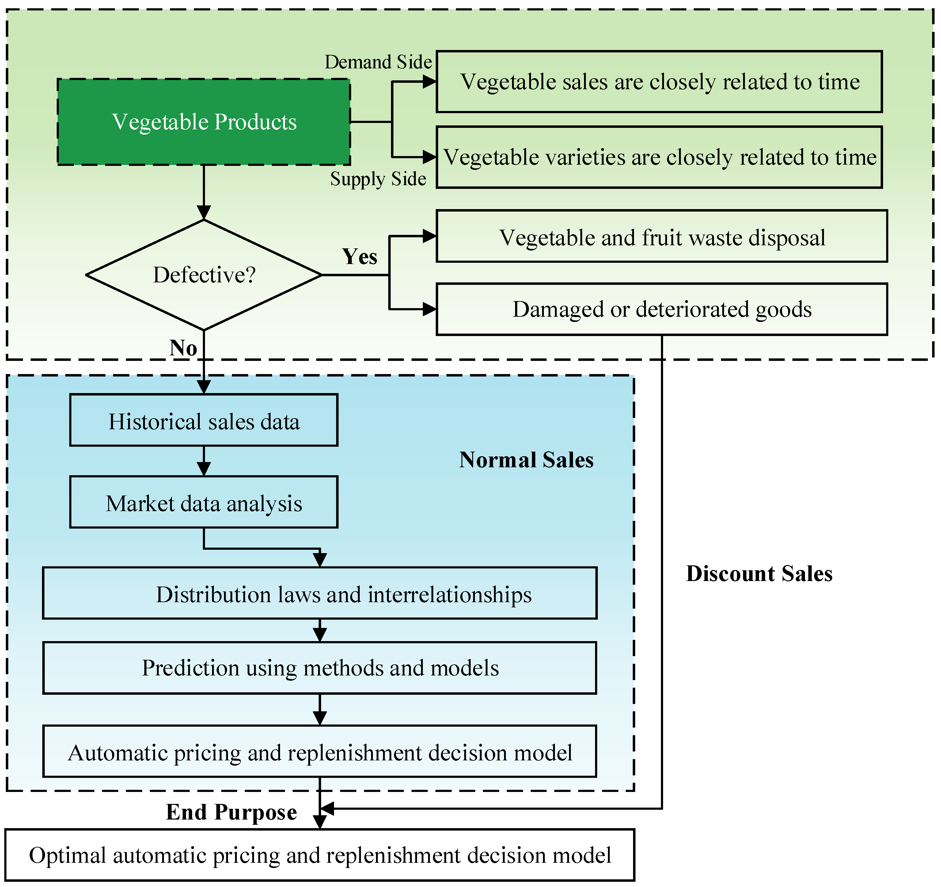
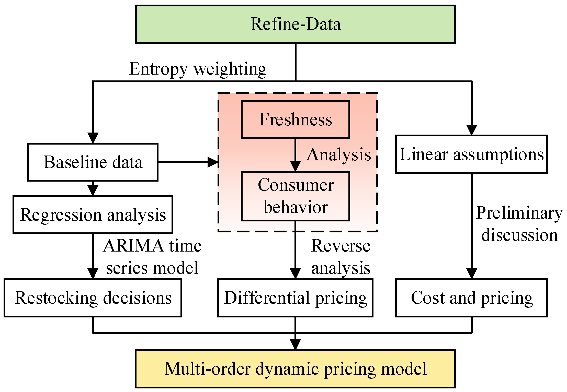
3. Materials and Methods

3.1. Analyzing Correlations in Vegetable Sales

The primary aim of analyzing correlations among various vegetable categories or individual items is to decode consumer demand and purchasing patterns through the analysis of sales volume distributions. This investigation reveals crucial insights such as product popularity, emerging sales trends, consumer preferences, and sensitivity to pricing among different vegetables. By leveraging these insights, supermarkets can refine their product mix optimization strategies, examining the sales distribution and exploring the interrelationships between different categories and individual vegetable products.
To deepen our understanding of these correlations, Spearman correlation analysis is employed [23]. This non-parametric statistical method is ideal for assessing the interdependence between two variables, especially when the dataset lacks repetitive values and exhibits a perfectly monotonic relationship between them, leading to a Spearman correlation coefficient of either +1 or −1. The detailed steps of this calculation process are outlined below:
Step 1: Rank Calculation. Organize the observations in each category by size and assign them corresponding ranks  R ( x )  and  R ( y ) . If identical observations occur, give the average of the ranks  R ¯ ( x )  and  R ¯ ( y ) .
Step 2: Difference Calculation. For each pair of ranks, calculate the difference between the ranks of the two categories and sum the squares of these differences.
Step 3: Spearman’s Correlation Coefficient Calculation. The Spearman’s correlation coefficient  R s  is calculated as follows:
R s = 1 n i = 1 n R ( x i R ¯ ( x ) ) · ( R ( y i ) R ¯ ( y ) ) 1 n i = 1 n R ( x i ) R ¯ ( x ) 2 · 1 n i = 1 n R ( y i ) R ¯ ( y ) 2
where n denotes the total number of samples, given that the target sample size in this study is substantial, a simplified formula is employed to calculate the sales volume of each vegetable category. This approach ensures the statistical robustness and reliability of the analysis.
r s = 1 6 i = 1 n D i 2 n ( n 2 1 )
where  D i  represents the difference in the ranks of the ith data pair. This calculation is integral to determining the correlation between two variables, especially when assessing the relationship between different categories in vegetable sales volume.
Step 4: Assessing Correlation Strength. The range of Spearman’s correlation coefficient is between −1 and 1. A value near 1 indicates a strong positive correlation between the two categories, suggesting that as one variable increases, so does the other. Conversely, a value close to −1 signifies a robust negative correlation, indicating that as one variable increases, the other decreases. A coefficient near 0 also suggests little to no linear correlation between the categories.
Step 5: Determining Correlation Significance. Employ hypothesis testing to evaluate the significance of the correlation. This involves comparing the calculated p-value with a predetermined significance level, often denoted by an asterisk (*). A p-value lower than the significance level suggests that the observed correlation is statistically significant, whereas a higher p-value indicates that the correlation might have occurred by chance.
This study revealed significant positive correlations among specific vegetable categories via case analysis. The findings suggest that enhancing sales links between these categories during both the sales and restocking phases could be beneficial. To extend beyond mere correlation analysis, the study utilized the Q-clustering algorithm. This unsupervised learning method seeks to unveil the intrinsic structure of data by identifying and categorizing highly similar objects. It computes the Euclidean distance between each data point and its respective cluster center, thus effectively capturing the subtle nuances within this multidimensional space. Such an approach not only refines data analysis and interpretation but also deepens our understanding of the underlying relationships and patterns within the vegetable sales data.
Assuming there are N types of individual vegetable items that can be classified into K categories in total,  C 1 , C 2 , , C k , let  V t i  represent the ith attribute value in the category  C t , N t  denote the number of attribute values in  C t , and  V ¯ t  mean the center of mass of  C t . The specific formula for calculating the Euclidean distance is provided as follows:
d ( C , V ¯ t ) = t = 1 N ( C t V t i ) 2 , ( 1 t k )
The Sum of Squares of Departures (SSD) is introduced to evaluate the clustering quality across the entire dataset. Based on the earlier description of the multidimensional data space, the sum of squares of deviations for individual vegetable species and the K categories are calculated.
S t = i = 1 N t ( V t i V ¯ t ) T ( V t i V ¯ t )
S = t = 1 K i = 1 N t ( V t i V ¯ t ) T ( V t i V ¯ t )

3.2. Replenishment Model
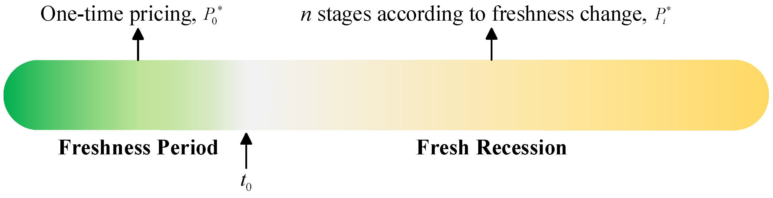
To meet consumer demand and ensure shelf availability, fresh food retailers, such as hypermarkets, often restock large quantities of perishable vegetables. However, this practice frequently leads to significant losses because of high deterioration rates. Additionally, maintaining freshness in both shelving and storage areas is crucial. Although shelving units have freshness preservation tools in supermarkets and similar retail settings, maintaining strict control over temperature and humidity remains challenging. Products on shelves, directly accessible to consumers, are more susceptible to accelerated spoilage due to potential undesirable purchasing behaviors. In contrast, storage conditions are generally more controlled and stable. Considering the substantial seasonal and volatile vegetable sales data, this study initially developed an autoregressive integrated moving average (ARIMA) model [14] for predicting vegetable replenishment.
1 1 L 2 L 2 p L p ( 1 L ) d X t = 1 θ 1 L θ 2 L 2 θ q L q ε t , t = 2 , 3 , , n
In the ARIMA(p, d, q) model, the variables are defined as follows: Xt is the actual value, L represents the backward shifting operator, d denotes the constant term,  ε t  symbolizes white noise, and  p  and  θ q  are the model’s coefficients, estimated via the least squares method. The optimal ARIMA model is selected based on the Akaike Information Criterion (AIC). Constructing the ARIMA model for forecasting sales data involves several steps:
Step 1: Stationarity Test. Evaluate the stationarity of the original data. Apply differencing if the data are non-stationary. After first-order differencing, reassess stationarity. If still non-stationary, continue differencing until achieving stationarity.
Step 2: Parameter Identification. Determine the ARIMA model’s main parameters. The differencing count,  d , is established in Step 1. Parameters p (autoregressive) and q (moving average) are identified by examining autocorrelation and partial autocorrelation functions. The AIC is used for model selection, with lower AIC values indicating better model predictive performance.
Step 3: Residual Analysis. Post parameter identification, examine if the model’s residuals conform to a white noise sequence. Consistency indicates a well-fitted model. If inconsistency is found, reevaluate and adjust the model’s parameters.

3.3. Pricing Model

In addressing the challenges of category-based replenishment planning for vegetables, it is important to recognize that while unit sales data pertain to individual items, the planning focus should be on categories. Relying on unit sales prices for direct modeling could diminish the model’s explanatory power. Consequently, this paper aims to establish baseline sales figures for each vegetable category that reflect each product’s intrinsic value.
To accomplish this, we employ the entropy weight method, an objective technique that assesses the uncertainty and diversity of various indicators. This method calculates the information entropy of each indicator and assigns weights accordingly. Indicators that exhibit greater dispersion receive higher weights, aligning the model’s results more closely with reality. This specific weighting process is tailored to accurately reflect the interrelationships between sales and prices across different vegetable categories, enhancing our understanding of market dynamics. The specific weighting process is as follows:
Step 1 [23]: Normalization of Unit Sales Price. Normalize the unit sales price of each vegetable item for positive indicators using the formula:
z i j = x i j x min x m a x x min
For negative indicators:
z i j = x max x i j x m a x x min
Here,  z i j  is the normalized data, and  x min  and  x max  are the maximum and minimum values of each indicator, respectively.
Step 2: Weight Calculation for Each Metric. Calculate the weight of the jth metric in the ith unit sales price, approximated as the probability  p i j  in calculating the information entropy.
p i j = z i j i = 1 n z i j
Step 3: Information Entropy Calculation. Compute the information entropy  e j  of the jth indicator. Since a larger information entropy implies less information conveyed by the indicator, the corresponding utility value  d j  is calculated. Introduce a logarithmic function for conversion to measure the positive information quantity:
e j = 1 ln n i = 1 n p i j ln ( p i j )
Step 4: Redundancy Difference Calculation. Determine the redundancy difference in the information entropy of the jth item, reflecting the uniqueness and significance of each indicator.
d j = 1 e j
Step 5: Weight Assignment for Unit Price. Calculate the weight of the unit price of each vegetable item relative to the overall vegetable category. This step aggregates the weighted contributions of individual items to determine their collective impact on the category’s pricing.
w j = d j j = 1 m d j
In vegetable sales, consumers assess product freshness based on appearance, quality, and decay. When freshness falls below expectations, consumer purchasing interest declines significantly. Consequently, supermarkets often reduce prices to stimulate demand, increasing the sales volume of vegetables and maximizing sales profits. This paper categorizes the sales cycle into ’fresh’ and ’freshness decline’ periods, with  t 0  marking the transition. During the fresh period (before  t 0 ), vegetables remain largely untouched with minor freshness changes, warranting a single pricing event. Post  t 0 , in the freshness decline period, vegetables show signs of rotting. Therefore, dynamic pricing based on changes in freshness and consumer preferences is essential. Figure 2 illustrates the proposed dynamic pricing process.
This study accounts for the freshness variability of vegetable products and consumer time preferences by adopting a product-type function as the demand function for the vegetable market at a given time. This approach more accurately captures market demand uncertainty. The demand at a specific time is denoted as:
v d = m ( t ) P c Q
where  m ( t )  represents the consumer preference function relative to freshness changes;  P  is the baseline selling price for the vegetable category;  c  indicates the consumer’s price sensitivity coefficient; and  Q  is the initial demand at each sales stage.
The sales cycle  T  is segmented into  n  distinct stages for dynamic pricing. Each vegetable product’s freshness period is denoted by  ( 0 , t 0 ] . Once sales duration surpasses  t 0 , the product enters the freshness decline phase, further divided into two stages, each represented  ( t i 1 , t i ]  as illustrated in Figure 2. The paper employs a continuous exponential function to model the variation in consumer preference over time as follows:
m ( t ) = 1 ,                         t ( 0 , t ] e ( a ( t t 0 ) ) ,       t ( t i 1 , t i ]
where  a  is the freshness change factor; subsequently, substituting  m ( t )  into the demand function yields the demand  v d :
v d = P c Q 0 ,                               t ( 0 , t 0 ] e ( a ( t t 0 ) ) P c Q i ,     t ( t i 1 , t i ]
Upon determining the demand at a specific time, an integral approach is employed to calculate the demand within a phase  D i . Subsequently, the market demand for vegetable products across these various phases is aggregated to ascertain the total market demand for the entire sales cycle  D s s :
D s s = 0 T v d d t = P c Q 0 0 t 0 1 d t + P c Q 1 t 0 t 1 e ( a ( t t 0 ) ) d t + + P c Q n t n 1 t n e ( a ( t t 0 ) ) d t           = D 0 + D 1 + + D n           = P c Q 0 t 0 + i = 1 n 1 a ( e a ( t i 1 t 0 ) e a ( t i t 0 ) ) P c Q i
The demand for vegetable products during the freshness period  D 0  and for each stage of the freshness decline period  D i  is simplified and expressed as follows:
D 0 = γ 0 Q 0 D i = γ i Q i γ 0 = P c t 0 γ i = 1 a ( e a ( t i 1 t 0 ) e a ( t i t 0 ) ) P c

4. Results and Discussion

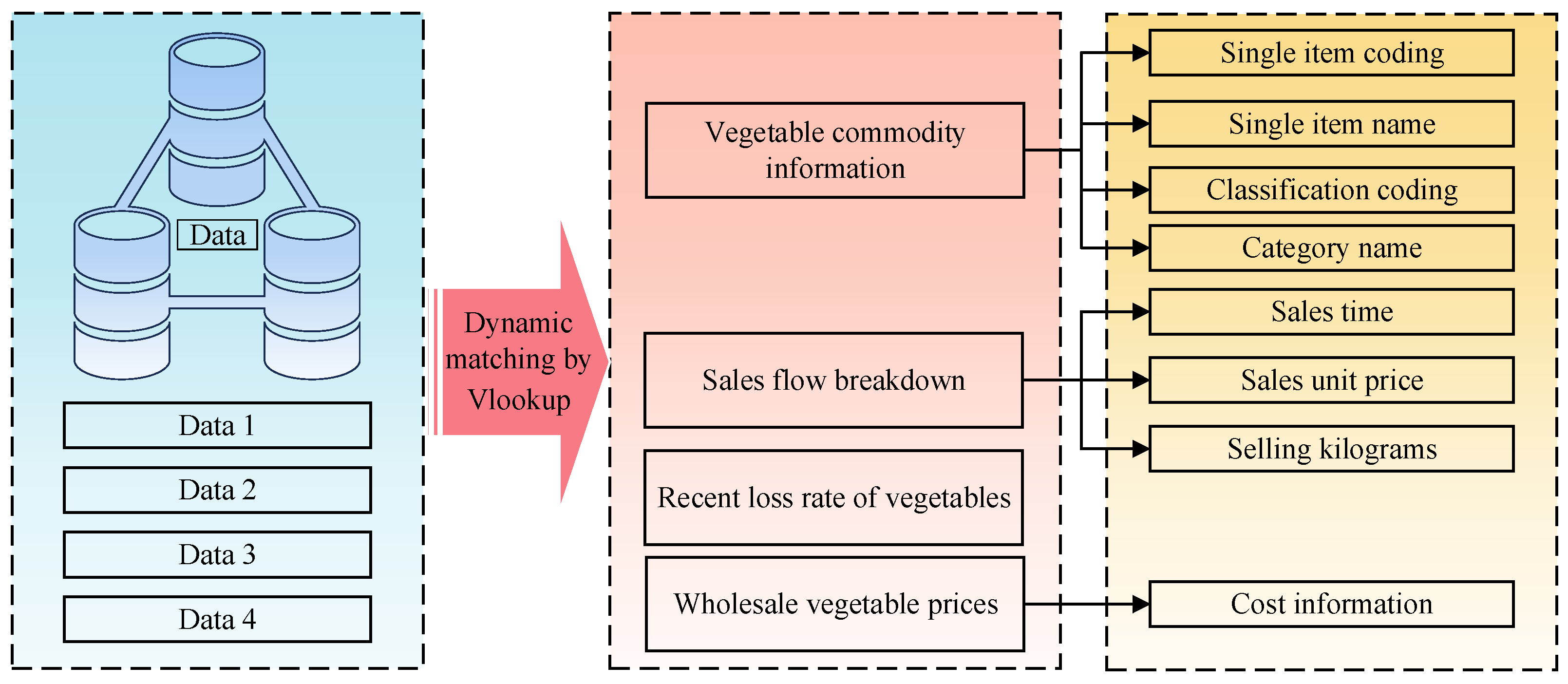
4.1. Data Pre-Processing

The data utilized in this study originate from the 2023 Chinese Contemporary Undergraduate Mathematical Contest in Modeling, Problem C [49]. Table 1 presents the number of individual vegetable items within the vegetable category group, as per the data source.
Given that the data originate from the specific sales figures of fresh food superstores, what might appear as abnormal sales data could be underpinned by unique real-world contexts. Thus, indiscriminate data cleansing could result in significant analytical biases. The study employs a more nuanced approach to data cleaning and processing to address this. It utilizes the VLOOKUP function to dynamically match information across various data sources, followed by pivot tables to distill specific information from large datasets. This method aims to preserve the real-world environment’s characteristics as much as possible while disregarding extraneous factors, as illustrated in Figure 3. Data 1 lists six vegetable categories encompassing 251 items, with a hierarchical relationship between items and their respective categories. Table 1 details the number of items per category. Data 2 offers comprehensive consumption data over three years, including unique codes for vegetable items and categories, types of sales and discounts, sales volume, and unit price for each item. Data 3 presents daily wholesale prices categorized by vegetable item codes. Data 4 provides specific wastage rate details for each item, identified by name.
The research initially focuses on summarizing vegetable category goods flow data from Data 2. It aggregates sales volume data across yearly, monthly, and daily dimensions to identify statistical patterns and correlations. Key statistical indices such as mean, median, standard deviation, maximum, minimum, peak, skewness, and dispersion coefficient are utilized. To visualize data distributions and trends, histograms and scatter plots demonstrate the scattering range and central position of each continuous data group. These visualizations help clarify the distribution and volatility of sales volumes. Further, the analysis leverages Spearman correlation to investigate relationships among vegetable categories. Subsequently, a clustering algorithm examines the connections between individual vegetable products, exploring their similarities and differences. This process highlights potential substitutive or complementary relationships among categories and products. The insights derived from this analysis provide guidance for superstores on optimizing display volumes. These decisions are informed by likely shopping basket combinations, influenced by strong correlations among categories and products. The analysis process and its findings are detailed in Figure 4.

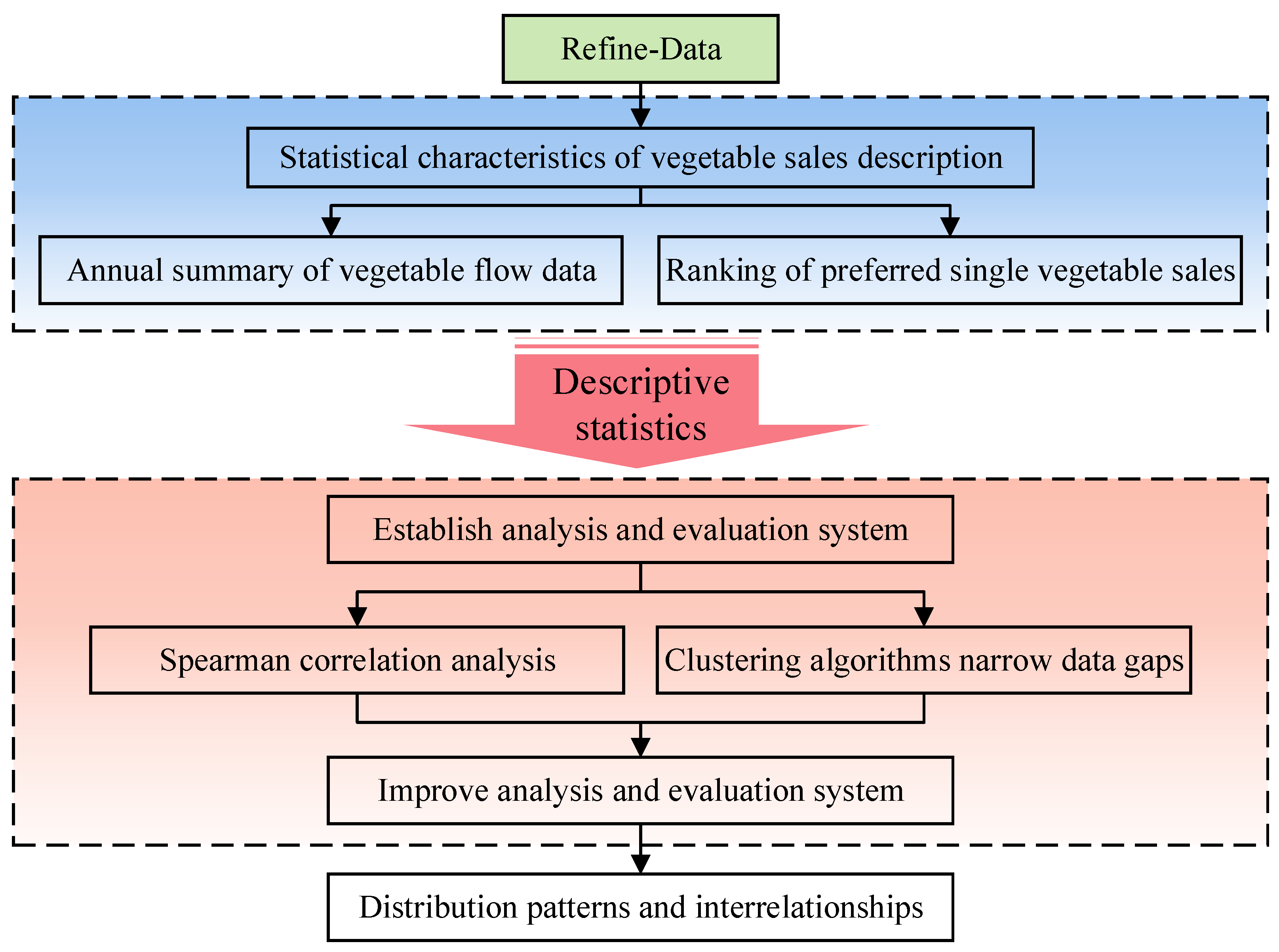
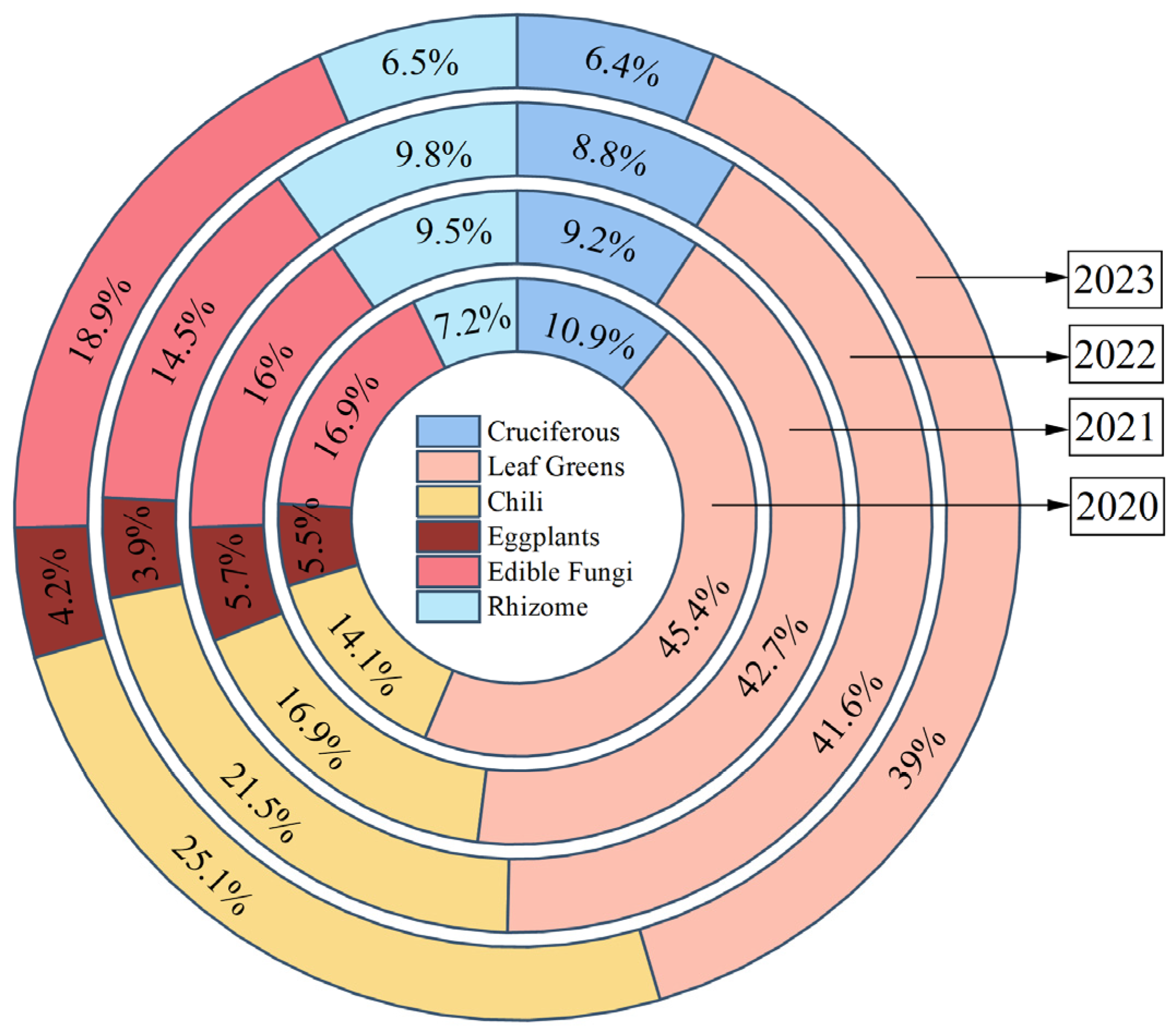
4.2. Descriptive Statistics and Correlation Analysis of Vegetable Sales Status

The core objective in examining correlations among different vegetable categories or individual products lies in understanding consumer demand and purchasing behaviors through the distribution patterns of sales volume. This analysis sheds light on crucial aspects such as the popularity, sales trends, consumer preferences, and price sensitivities of various vegetables. Supermarkets can enhance their product mix optimization strategies by delving into the sales volume distribution and the interrelationships between various categories and individual vegetable products.

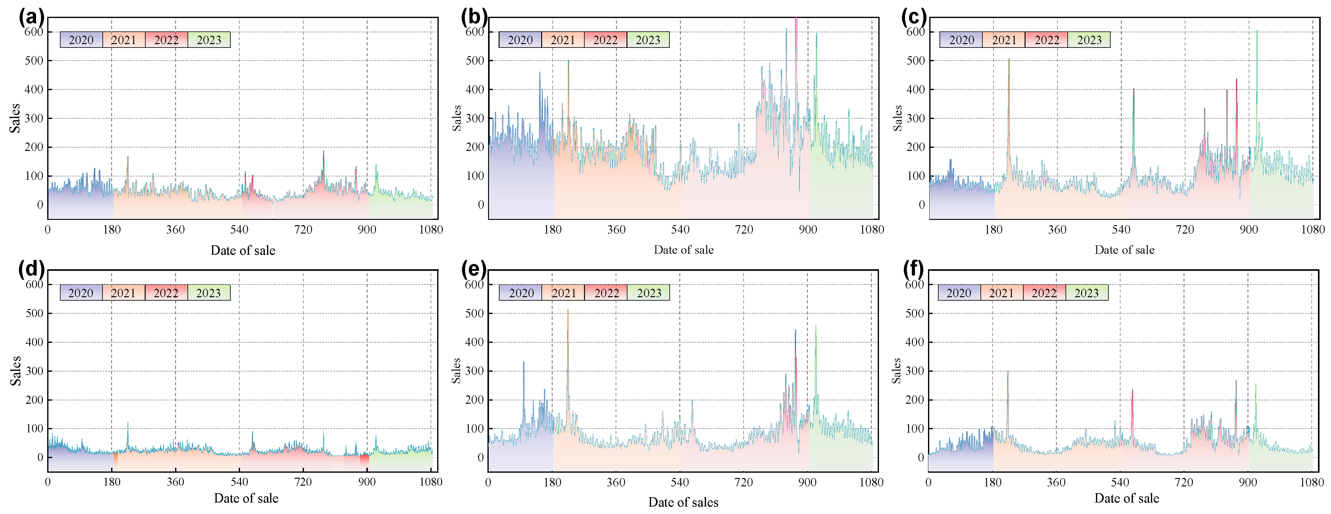
4.2.1. Sales Volume Distribution Patterns

To understand the role of each vegetable category in superstore sales and the evolution of their sales proportions, Figure 5 depicts the contribution of each category to total sales. The vegetable sales data span from 1 July 2020 to 30 June 2023. While data are available for only six months of 2020 and 2023, and there are no sudden shifts in the sales proportion of vegetable categories, this analysis assumes a relative homogeneity in the missing data. This assumption aims to avoid intricate data repair and filling procedures, thereby simplifying the analytical process.
Figure 5 arranges the sales data for different years concentrically, from the innermost to the outermost sectors. Over the years, leafy greens and vegetables have consistently been the top-selling category, sometimes contributing nearly 50% to total sales. However, since 2020, there has been a gradual decline in their sales share, with chilis and edible fungi ranking second and third, respectively. Cauliflowers and rhizomes exhibit similar sales shares, while eggplant vegetables record the lowest.
Figure 6 demonstrates the performance of each category throughout the sales cycle, showcasing daily sales volumes. Utilizing Pivot Tables, large-scale data are flexibly filtered and analyzed in detail to evaluate the overall sales status of each category. Furthermore, the analysis of daily sales data provides a deeper insight into consumer preferences and consumption habits for different vegetable categories, highlighting the distribution patterns of total sales volume for each category.
At a macro level, there is a discernible correlation in sales volume across six vegetable categories. From July 2020 to 2022, each category exhibited distinct evolutionary patterns. During June to August, a period characterized by robust vegetable growth due to adequate supply and quality, sales volumes for cauliflowers, leafy green, edible fungi, chilis, and rhizomes surged, peaking rapidly. Post-August, however, a pronounced downward trend in sales volumes was observed. Notably, with the lowest sales volume, eggplant vegetables displayed year-round fluctuations heavily influenced by seasonality, particularly during early spring when sales spiked. Leafy green vegetables led in sales across all categories. This category, with the most extensive variety, encompassing 100 individual types, offers consumers a wide range of choices. Their diversity, catering to varied consumer needs and being staple ingredients in home cooking, significantly drives total sales growth. The analysis and ranking of sales volumes of individual vegetable items delved deeper into consumer preferences. Figure 7 reveals that Wuhu green pepper, broccoli, and lotus root topped the sales, each exceeding 27,000 kg, signifying high consumer preference. Chinese cabbage, ranking fourth, had a sales volume of 19,187 kg, with the sales of other individual items decreasing in line with their rankings.
To thoroughly analyze the characteristics and variations in sales data, this study examines the statistical patterns of sales volume for each vegetable category. These patterns include mean, median, standard deviation, maximum, minimum, kurtosis coefficient, skewness coefficient, and dispersion coefficient. The kurtosis coefficient ( γ p ) measures the peakedness of the data distribution, reflecting the sharpness of the peak and the heaviness of the tails. It is calculated by dividing the fourth central moment of a distribution by the square of its variance and then subtracting 3. This adjustment sets a normal distribution as a reference, aligning it to a relative scale. Interpretation of the kurtosis coefficient is as follows:
When  γ p = 0  the distribution resembles a normal distribution.
When  γ p > 0  the distribution is more peaked with narrow tops and heavy tails; it indicates a leptokurtic distribution.
When  γ p < 0  the distribution is flatter with gentler peaks and shorter tails; it denotes a platykurtic distribution.
The formula for calculating the kurtosis coefficient is:
γ p = h 4 h 2 2 = E X E ( X ) 4 V a r ( X ) 2 3
where  V a r ( X )  represents variance,  E ( X )  indicates mean, and  h n  denotes the nth order central moment. Using these variables, we can accurately analyze and describe the distribution characteristics of vegetable sales data, leading to a deeper understanding of the statistical patterns of sales volume across different vegetable categories.
The skewness coefficient ( γ s ) is a measure of asymmetry in the data distribution, assessed through the probability density function curve of a random variable:
When  γ s = 0  the data distribution is symmetrical.
When  γ s > 0  the data distribution is right-skewed; it indicates a longer or fatter tail on the right side.
When  γ s < 0  the data distribution is left-skewed; it means a longer or fatter tail on the left side.
The formula for the skewness coefficient is:
γ s = h 3 h 2 3 2 = E ( X E ( X ) ) 3 [ V a r ( X ) ] 3 2
The Coefficient of Variation (CV) is a statistical tool used to measure the dispersion within a dataset. Its utility lies in enabling comparisons of dispersion across different datasets, irrespective of their units or mean values. Defined as the ratio of the standard deviation ( σ X ) to the mean ( m X ), CV describes the relative variability of a dataset. The formula for calculating CV is:
CV = σ X m X × 100 %
An extensive CV value indicates a high degree of dispersion, signifying a more significant fluctuation of the data points relative to the mean. On the other hand, a small CV indicates a low degree of dispersion, signifying that data points cluster more tightly around the mean.
Table 2 presents descriptive statistics for the total sales of six vegetable categories, focusing on skewness and kurtosis coefficients. The skewness coefficient assesses data distribution asymmetry; a coefficient greater than zero indicates a right-skewed distribution, with most data falling left of the mean. Eggplants and cruciferous exhibit skewness coefficients near 0, suggesting relatively symmetrical sales distributions. The kurtosis coefficient describes the peak of data distribution. Cruciferous, eggplants, and rhizomes, with kurtosis coefficients less than zero, display flatter peaks and shorter tails than a normal distribution, indicating a platykurtic pattern.
Conversely, leafy greens, chilis, and edible fungi, with coefficients more significant than zero, have sharper, more peaked distributions with thicker tails, indicative of a leptokurtic pattern. Specifically, cruciferous, eggplants, and rhizomes exhibit near-negatively skewed distributions, and chilis and edible fungi align closely with normal distributions. Notably, the mean and median for the leafy green category are substantially higher than other categories, highlighting its highest consumer demand.

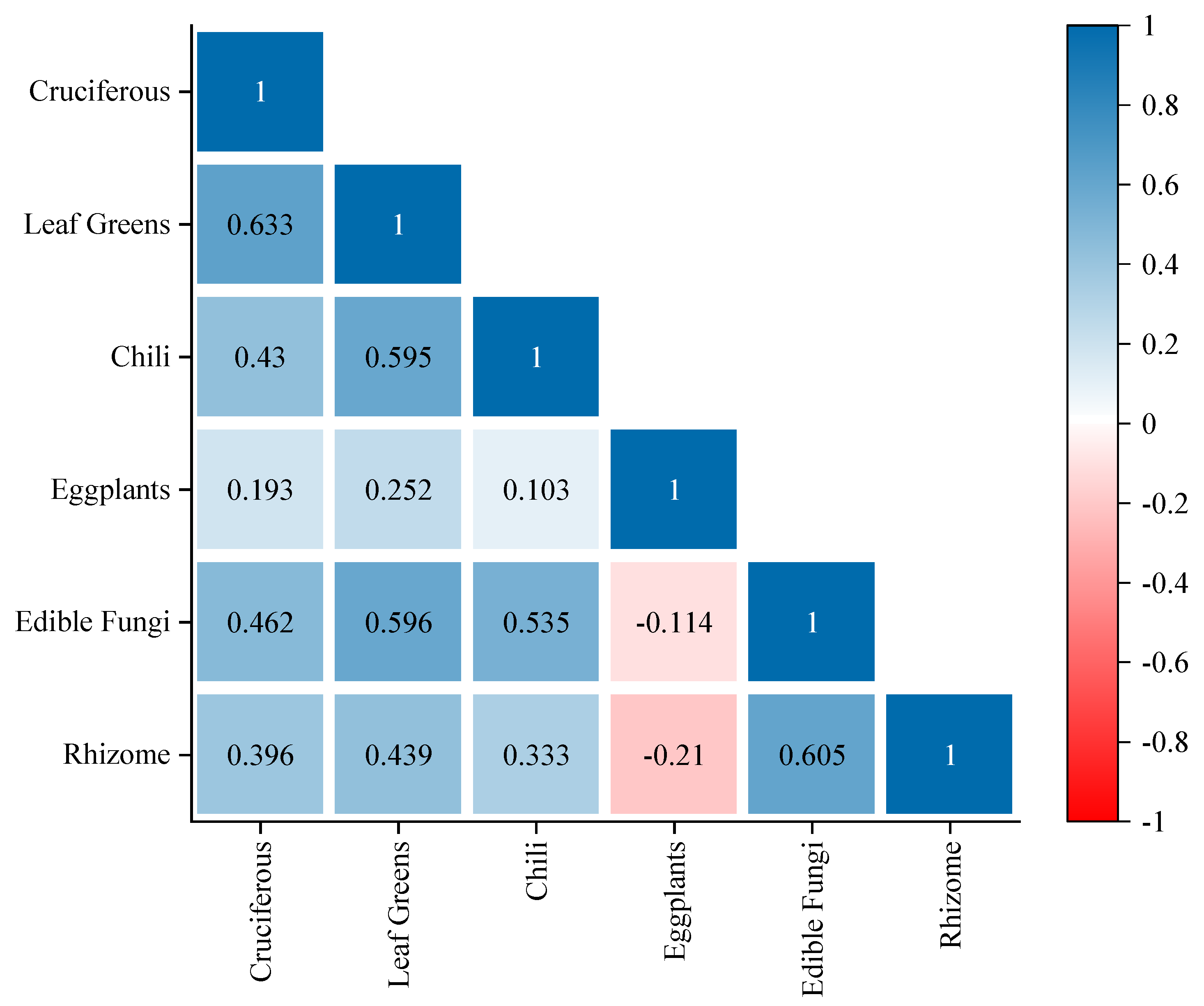
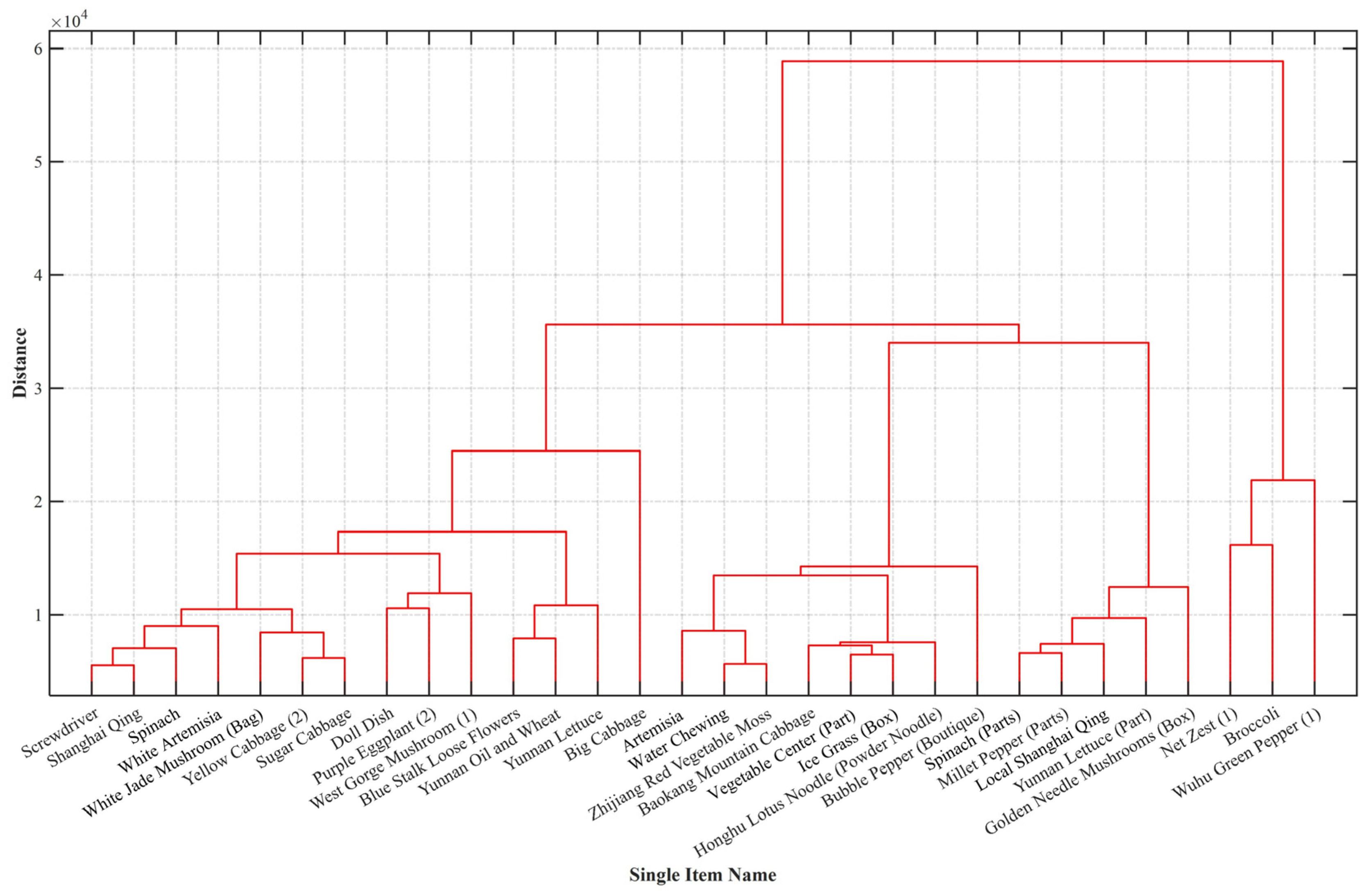
4.2.2. Correlation between Category and Individual Item

Spearman correlation analysis is a non-parametric statistical method used to evaluate the interdependence between two variables by calculating their correlation [23]. When the data contain no repetitive values, and a perfectly monotonic relationship between the two variables exists, the Spearman correlation coefficient will assume a value of +1 or −1.
Spearman’s correlation analysis was performed on six vegetable categories, with results presented in Figure 8. The analysis revealed varied correlations among these categories. Cauliflowers and leafy vegetables were prominent, distinguished by their broad assortment of items and substantial annual sales volumes. A strong positive correlation was noted between the remaining vegetable categories and both cauliflower and leafy vegetables, suggesting opportunities to enhance total sales via cross-selling strategies. In contrast, the presence of a negative correlation necessitates targeted adjustments during the replenishment process to optimize sales.
Further in-depth analysis revealed a significant positive correlation between cauliflower and foliar categories, with a correlation coefficient of 0.633. This finding suggests that enhancing linkage sales opportunities between these two categories could be beneficial during the sales and replenishment phases. However, it is essential to note that eggplant vegetables negatively correlated with edible mushrooms, aquatic roots, and tubers, indicating different consumer purchasing patterns. Let us extend beyond mere correlation analysis to employ the Q-clustering algorithm. Q-clustering, an unsupervised learning method, uncovers the intrinsic structure of data by identifying and categorizing objects that exhibit high degrees of similarity. This application constructed a data space encompassing the sales volume of 251 vegetables. The algorithm effectively captures the nuances in this multidimensional space by calculating the Euclidean distances between data points and their respective clustering centers. This approach allows for more precise data analysis and interpretation, offering more profound insights into the relationships and patterns within the vegetable sales data.
The model aims to minimize the loss-based metric, precisely the sum of squared deviations. Initially, each sampling point is treated as a separate category. When merging categories, it prefers to merge those two categories that minimize the increase in the sum of squared deviations. This process repeats until all sampling points are grouped into a single category. The Q-clustering algorithm presents its results in Figure 9, providing structured insights into the relationships and groupings of various vegetable types based on their sales data attributes.
The clustering results depicted in Figure 9 enable the categorization of vegetable items into three principal groups:
(1)
Home-cooking vegetables. This category includes staples like Chinese cabbage. These vegetables are diverse, high in volume, and commonly used in home cooking, indicating a steady supermarket demand. This category may necessitate strategies focusing on mass production and supply to meet consistent consumer needs.
(2)
Common side dish vegetables. Encompassing vegetables like lotus root, broccoli, and Wuhu green peppers, these are characterized by their nutritional richness and frequent use in side dishes across various cuisines. The variety of dishes incorporating these vegetables could result in higher purchasing demand from food manufacturers and caterers.
(3)
Specialized demand vegetables. The third category features vegetables with a smaller gap between their use in dishes and their sales volumes. While the market demand for these vegetables might not be as robust as the first two categories, they cater to specific consumer groups, indicating a niche market.
Clustering sales data attributes enables clear insights into the structured relationships and grouping of vegetable sales. This allows for understanding the sales characteristics of various vegetable categories and consumer demands, facilitating improved market segmentation and identification of market positioning. Such insights offer guidance for developing tailored inventory and marketing strategies, as well as devising more effective inventory management and marketing approaches, thereby informing corresponding business strategies.

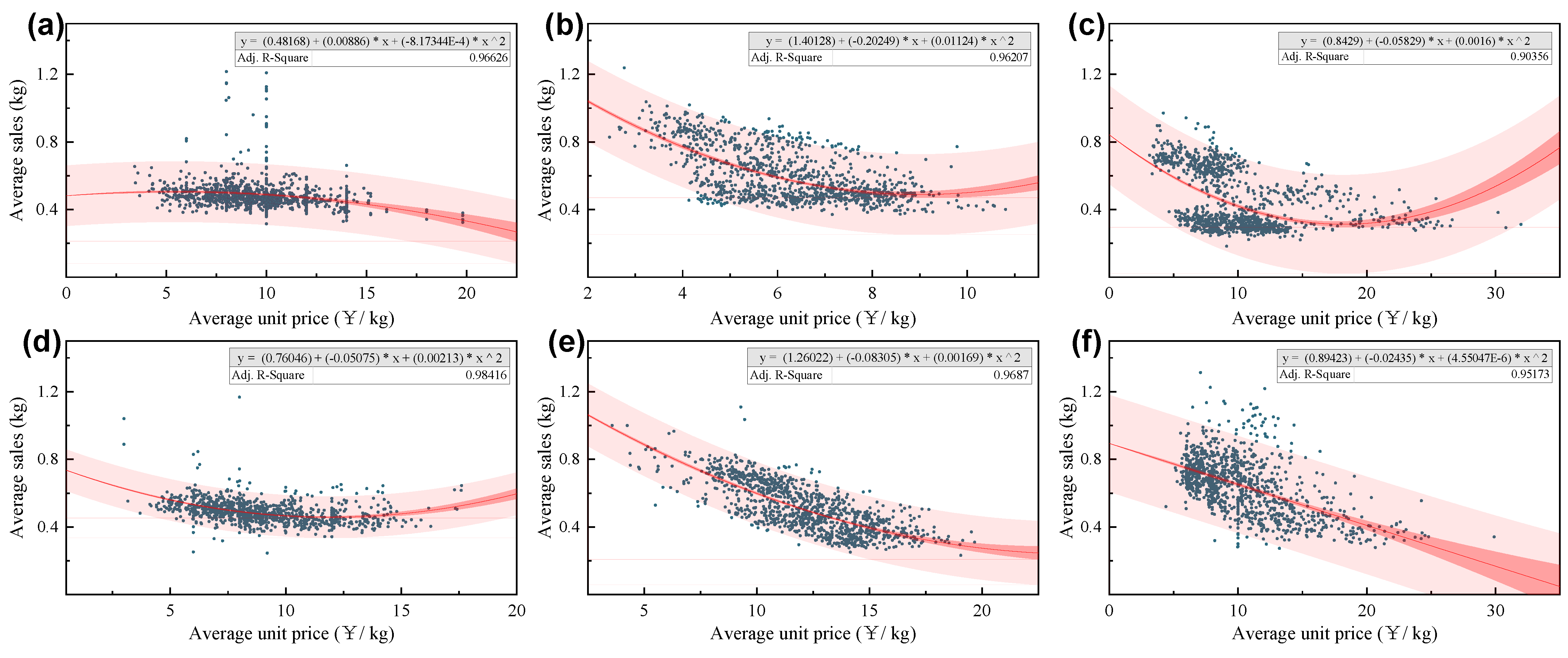
4.3. Strategy Analysis in the Pricing Model

To maximize revenue, developing a well-conceived dynamic pricing strategy is essential. This strategy transcends mere product factor considerations; it fundamentally addresses a planning challenge focused on effectively mitigating or disregarding the influence of confounding factors. Examination of the detailed sales data from Data 2 reveals a cost-plus approach to determining sales unit prices. Since the prices are intricately tied to individual vegetable items, conducting an item-by-item analysis would be cumbersome and inefficient. Therefore, replenishment planning should focus on a category level, where integrating individual item values within each category presents a significant challenge.
The initial step involves pre-processing and uniformly simplifying the complex category data. An entropy weighting method is then used to assign weights to each item’s average daily sales volume within a category, determining the item’s contribution to the overall sales volume. This approach effectively streamlines the workload by transforming granular unit price data into more manageable category-level benchmark data. After pre-processing, regression analyses are conducted for each category. Quadratic polynomial regression is employed to uncover the intrinsic relationship between total sales and pricing, given the limitations of simple linear regression in capturing real-world data complexities.
In examining pricing strategies, this analysis initially employs a linear framework derived from the cost-plus model to elucidate the relationship between cost and pricing. The study incorporates consumer purchasing behaviors, specifically emphasizing product freshness as a pivotal element for retrospective analysis. It segments the sales cycle by product freshness, facilitating variable pricing, particularly during periods of freshness deterioration. This segmentation supports the development of a dynamic planning model that adapts to changes in product freshness. Moreover, the quantum particle swarm algorithm plays a crucial role in identifying the optimal parameters necessary for executing a multi-tiered, dynamic pricing strategy. Detailed methodologies and analytical approaches are presented in Figure 10.
Overall, the scheme streamlines complex data processing and establishes precise weight distributions. Utilizing quadratic polynomial regression rather than simple linear regression more accurately captures the intricate inherent correlation between sales volume and pricing. The integration of consumer purchasing behavior and product freshness facilitates sales cycle segmentation and differentiated pricing that is aligned with freshness levels, enhancing the effectiveness and flexibility of sales strategies in response to market demand. The ultimately developed dynamic programming model comprehensively addresses the impact of freshness changes, optimizing pricing at various stages to maximize anticipated sales revenue.

4.3.1. Dynamic Adjustment Benchmark for Category Sales Unit Price

In addressing the challenge of replenishment planning by vegetable categories, it is crucial to note that while the sales data’s unit price is linked to individual items, the plan focuses on categories. As Figure 3 shows, there is significant variation in the number of particular items and their wholesale prices across different categories. Directly modeling using unit sales prices from Data 2 could diminish the model’s explanatory power. Consequently, this paper aims to construct benchmark sales for each vegetable category, reflecting the intrinsic value of each product. The entropy weight method, an objective weighting technique, is utilized to assess the uncertainty and diversity of each indicator. This method calculates the information entropy of each indicator and assigns weights accordingly. Indicators with more excellent dispersion will receive higher weights. Adjusting these weights ensures that the results align more closely with reality. Take the cruciferous category as an example; the paper selects the sales unit price of items such as green-stemmed cruciferous, broccoli, and purple cabbages (1 and 2) as positive indicators. Weights are assigned to these indicators to objectively represent the interconnection between sales volume and pricing across various vegetable categories.
Convert the individual sales price into the sales benchmark price of the vegetable category. Due to space constraints, the assignment results are demonstrated specifically for the cauliflower category, presented in Table 3. Items like Purple Cabbage 2 and Purple Cabbage 1 have higher weights, indicating a more significant impact on the category’s pricing strategy. Table 3 is crucial for understanding the pricing dynamics within the cruciferous category and informing strategic pricing decisions.
The prevalent business strategy in supermarket operations involves formulating replenishment plans and analyzing the relationship between total sales volume and cost-plus pricing on a category-by-category basis. This approach recognizes that vegetable sales volume is significantly influenced by price, exhibiting a non-linear pattern. A quadratic polynomial regression model is particularly effective in revealing this non-linear relationship. Its flexible fitting curve provides considerable explanatory power for these analyses.
Q i = β i 0 + β i 1 P i + β i 2 P i 2
Here,  Q i  represents the total sales volume of the ith vegetable category,  P i  denotes the sales benchmark price of the ith category, and  β i j  symbolizes the regression equation coefficients. This formulation allows for a nuanced understanding of how pricing strategies impact sales volumes, enabling more informed decisions in replenishment planning and pricing adjustments.
Figure 11 and Table 4 display the outcomes of quadratic polynomial regression analyses for all six vegetable categories. The results indicate a high degree of model fit across these categories, as evidenced by the coefficient of determination (R2) for each model exceeding 0.9. This high R2 value signifies that the models successfully capture the relationship between sales volume and other influencing factors. Particularly noteworthy is the eggplant category, which exhibited the best regression fit with the value of 0.9816. It implies that the model explains approximately 98.16% of the variance in sales volume changes for eggplants, demonstrating a remarkably high degree of model fit and explanatory power.

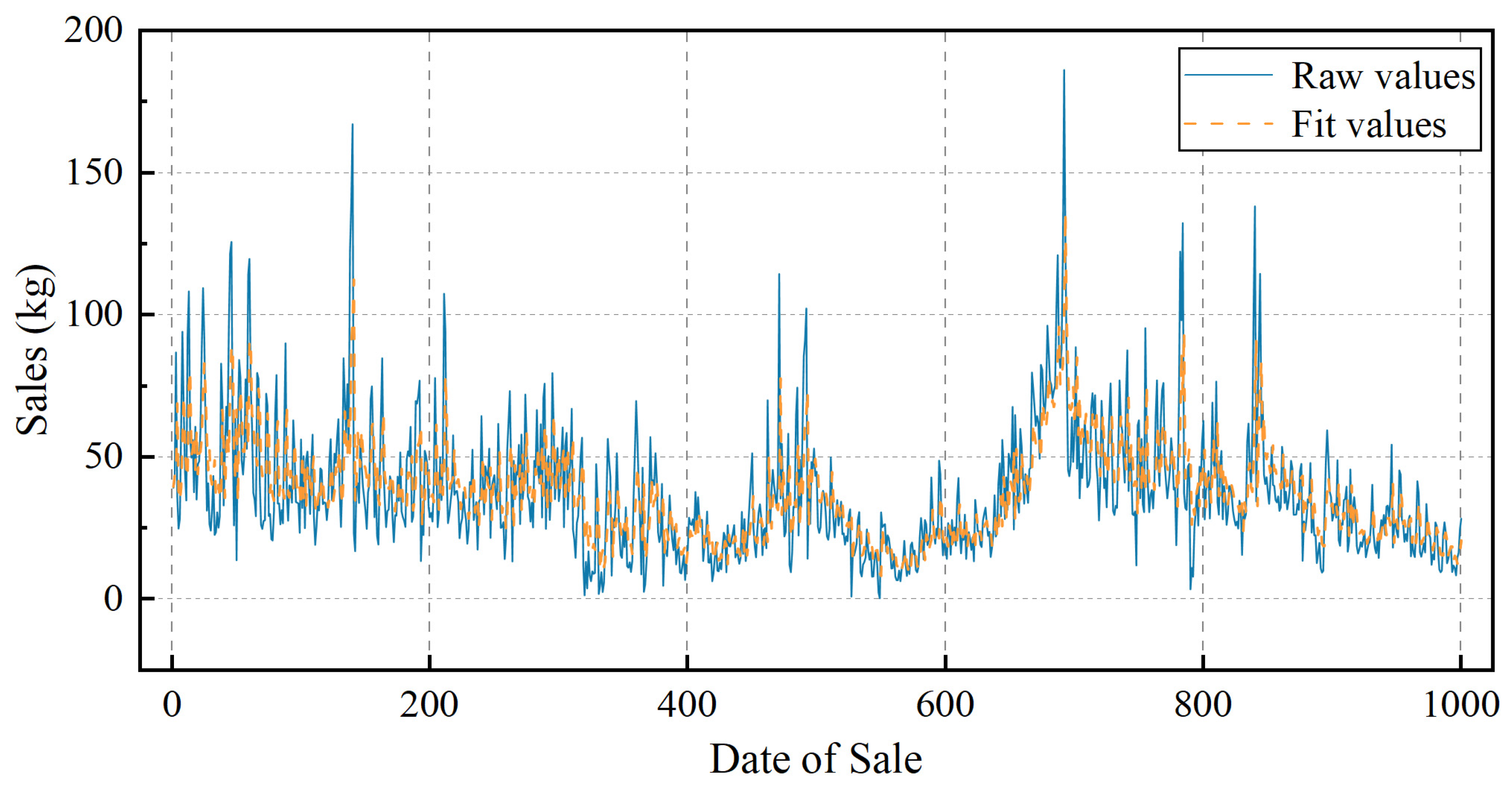
4.3.2. ARIMA-Based Replenishment Forecasting

Acknowledging the impact of white noise and random factors in sales data, the traditional autoregressive moving average (ARMA) model encounters challenges with non-stationary time series. Consequently, this study employs the ARIMA model, which incorporates a different step  d ( d 1 )  to convert non-stationary series into stationary ones, facilitating subsequent analysis and forecasting using the ARMA framework. This method effectively addresses the stochastic nature of parameters, thus greatly enhancing the model’s applicability. The ARIMA(p, d, q) model can be succinctly expressed as:
1 i = 1 p i L i ( 1 L ) d X t = 1 i = 1 q θ i L i ε t
where  L  represents the lag operator,  p  signifies the autoregressive period,  d  indicates the order of differencing, and  q  is the number of moving averages. By judiciously selecting the parameters of the ARIMA model, one can effectively fit the time series model and make probabilistic forecasts about the characteristics of its parameters. Table 5 displays the results of the Augmented Dickey–Fuller (ADF) test, a stability test applied to the sales volume data of the cauliflower category from the second half of 2020 to the first half of 2023. This test confirms the stability of the time series post differencing. Conversely, Figure 12 illustrates the ARIMA model’s fitting results for the sales volumes across various vegetable categories, showcasing the model’s applicability and effectiveness in capturing the dynamics of sales data.
To holistically account for the periodicity, seasonality, and stochasticity of the data, this study employs four metrics to evaluate the fitting accuracy and robustness of each forecasting model: Mean Absolute Percentage Error (MAPE), Root Mean Square Error (RMSE), Symmetric Mean Percentage Error (SMAPE), and Theil’s Inequality Coefficient (TIC). The comparative results in Table 6 show that the ARIMA model achieves a MAPE of 5.5253%, demonstrating strong performance in terms of mean absolute percentage error. The RMSE, SMAPE, and TIC values are below 5%, signifying high accuracy and stability in the model’s predictions. Utilizing the ARIMA model, Figure 13 presents the forecasted demand replenishment for various vegetable types from 1 July to 6 July, 2023. These predictions offer superstores a quantitative reference to anticipate and meet future demand effectively.

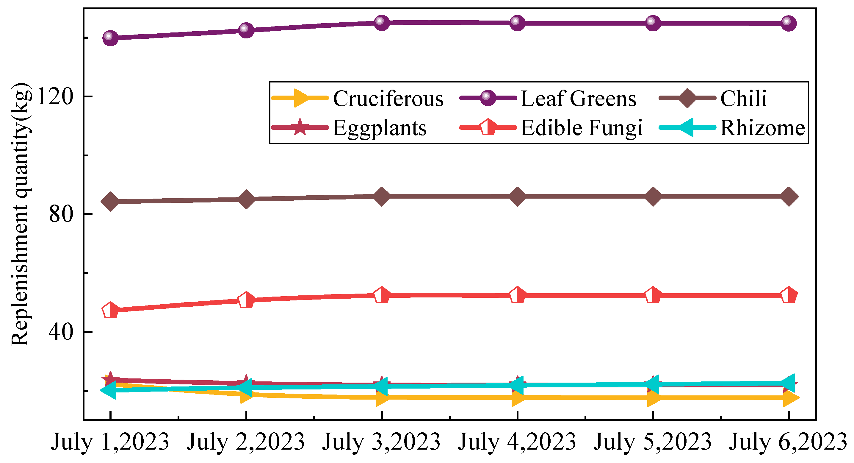
4.4. Multi-Order Dynamic Model

The conventional cost-plus pricing approach suggests pricing products to cover production and distribution costs, adding a profit margin. This paradigm emphasizes seller control over pricing, while the buyer’s influence mainly affects the markup rate, and begins with a linear hypothesis to explore the cost–pricing relationship:
P = ( 1 + w ) C
Integrating the regression relationship between sales volume and unit price for the vegetable category with the linearity assumption between cost and pricing leads to the development of the following planning model:
max P r o f i t = j = 1 m i = 1 n ( P i C i ) q i
s . t . Q i = β i 0 + β i 1 P i + β i 2 P i 2 P i = ( 1 + w i ) C i i = 1 , 2 , , 6 j = 1 , 2 , , 7 w i ( 0 , 0.5 )
Here,  P  represents the baseline selling price of the vegetable category,  C  is the baseline cost of goods sold,  Q  denotes the sales volume, and  w  is the cost-plus rate. It advances the linear pricing model by incorporating wastage rates and segments the sales cycle into multiple stages. This segmentation allows for systematic modeling of inventory changes throughout the sales period, aligning pricing strategies closely with product freshness and consumer demand dynamics. The product function describes the market demand for vegetable commodities at a specific time, considering the randomness of market demand. Assume that the initial demand for vegetable commodities at each stage obeys a uniform distribution of (0, M), and M is the maximum consumer demand for vegetable commodities in the superstore at each stage throughout the sales process. Further, to construct the expected quantity and profit function for the sales of the vegetable merchandise, a probability distribution function  f ( Q )  for the consumption demand is introduced, and the cumulative probability distribution function is denoted as  F ( Q ) . If the probability distribution function of the consumption demand D for the vegetable category at each sales stage is represented as  ϕ ( D )  then the following relationship can be established:
ϕ ( D ) = ϕ ( D ) D = 1 γ F ( Q ) Q = 1 γ f ( Q )
where  γ  is the demand coefficient. Considering the vegetable market demand, we can determine the expected sales volume  E S i  for the superstore at the ith sales stage ( t ( t i 1 , t i ] ). The introduced probability distribution function  f ( Q )  and the cumulative distribution function  F ( Q )  establish the following relationship:
E S i = 0 q i D i ϕ ( D i ) d D i + q i + q i ϕ ( D i ) d D i           = 0 q i γ i Q i f ( Q i ) d γ i Q i + q i γ i + q i γ i f ( Q i ) d γ i Q i           = q i γ i 0 q i γ i F ( Q i ) d Q i
Here,  q i  represents the order quantity of vegetable products at the ith sales stage. The first integral represents the expected sales volume when the market demand is less than or equal to the order quantity at that stage ( D i < q i ). The second integral corresponds to the expected sales volume when the market demand exceeds the order quantity ( D i q i ). Combining these two integrals can accurately calculate the expected sales volume for each stage.
When the order quantity  q i  surpasses the market demand  D i  for vegetables, surplus vegetable products are generated. This study calculates the expected surplus  E S U i  of vegetable products at each sales stage. It is assumed that the retailer orders  q 0  only once at the beginning of the sales cycle. The order quantity  q i + 1  in the ( i + 1 )th stage is set to equal the surplus quantity  E S U i  from the previous stage. This surplus variable is a crucial state variable in the dynamic pricing model, and its relationship equation is as follows.
E S U i = q i + 1 = 0 q i ( q i D i ) ϕ ( D i ) d D i = 0 q i γ i ( q i γ i Q i ) 1 γ i f ( Q i ) d γ i Q i = γ i 0 q i γ i F ( Q i ) d Q i
The equation adjusts the order quantity for the next stage based on the surplus from the current stage, optimizing inventory management and reducing wastage. Such dynamic adjustment is crucial in the dynamic pricing model, as it influences pricing strategies and inventory decisions in response to changing market demands. The analysis of the profit function is based on established expected sales and residual volumes. Assuming the retailer’s initial order quantity of vegetables is the unit price, and the retail unit price at each stage is defined accordingly, the profit function for vegetables is described as the total revenue from sales minus the initial order cost. This function reflects the total profit from vegetable sales, considering the staged change in freshness. The proposal includes a multi-order dynamic pricing model to maximize total profit, incorporating specific forms of the profit function, consumer demand coefficients, and their parametric variables. This model considers the influence of freshness changes on consumer preferences, enabling a more accurate representation of market dynamics and consumer behavior expressed by:
max Π ( P ) = i = 0 n P i ( q i γ i 0 q i γ i F ( Q ) d Q ) C q 0
s . t . γ 0 = P 0 c t 0 γ i = 1 a P i c ( e a ( t i 1 t 0 ) e a ( t i t 0 ) ) q i = γ i 1 0 q i 1 γ i 1 F ( Q ) d Q , i = 1 , 2 , , n P 0 = 2 M t 0 q 0 ( c + 1 ) c P i * = 2 M ( e a ( t 0 t i 1 ) e a ( t 0 t i ) ) a q i ( c + 1 ) c i = 1 , 2 , , n
The revenue  Π ( P )  is derived from the product of the selling price and the expected sales volume, influenced by several factors, which include the freshness change factor ( a ), the upper demand limit ( M ), the demand coefficient ( γ ), and the number of target segments ( n ). Heuristic algorithms, including genetic and particle swarm optimization, are known for their robust search capabilities and quick convergence. The quantum particle swarm optimization (QPSO) algorithm is notable for its stability, superior searchability, and rapid convergence. This research uses the QPSO algorithm to determine the optimal parameters within the model, especially in Equations (29) and (30). This approach aims to identify the most effective pricing and replenishment strategies. During the fresh period  t ( 0 , t 0 ]  for a vegetable category, the profit function is delineated as follows:
Π ( P ) = i = 0 n P i ( q i γ i 0 q i γ i F ( Q ) d Q ) C q 0
Calculate the first-order derivative of Equation (31) concerning  P 0  determining the optimal pricing. Furthermore,  γ 0  is expanded, allowing for the derivation of the first-order and corresponding second-order derivative expressions:
d Π ( P 0 ) d P 0 = q 0 ( c + 1 ) P 0 c q 0 2 2 M t 0
d 2 Π ( P 0 ) d P 0 2 = c ( c + 1 ) P 0 c 1 q 0 2 2 M t 0
The analysis reveals the price sensitivity coefficient  c > 0  for consumers regarding vegetable products, leading to  P 0 c 1 > 0 . Additionally, the upper limit of demand  M > 0 , implies the overall value  c ( c + 1 ) P 0 c 1 q 0 2 2 M t 0 < 0 . Consequently, the second-order derivative of the original profit function concerning  P 0  is denoted as  d 2 Π ( P 0 ) d P 0 2 < 0 . Therefore, when the first-order derivative equals zero, the optimal pricing  P 0  for vegetable products during the freshness period can be established. It is crucial for setting strategic pricing in the freshness period to maximize profits.
P 0 = 2 M t 0 q 0 ( C + 1 ) c
Substituting gives the fresh period profit function as:
Π 0 = 1 2 q 0 ( 2 C + 2 c 1 c + 1 ( M t 0 ( 1 + c ) q 0 ) 1 c ( 2 1 c ( M t 0 ( 1 + c ) q 0 ) 1 c ) c q 0 M t 0 )
As the vegetable product enters the freshness decline period  t ( t 0 , t n ] , the profit function for this phase is derived using a methodology akin to that of the fresh period:
Π i = 2 1 c ( M ( e a ( t 0 t i 1 ) e a ( t 0 t i ) ) ( c + 1 ) a q i ) 1 c q i ( 2 a ( 2 1 c ( M ( e a ( t 0 t i 1 ) e a ( t 0 t i ) ) ( 1 + c ) a q i ) 1 c ) c q i ( e a ( t 0 t i 1 ) e a ( t 0 t i ) ) M )
The Refine-data database documented 878,500 orders from the second half of 2020 to the first half of 2023. In this study, a day’s vegetable sales at the superstore, operating from 8:00 to 22:00, are considered a sales cycle. Acknowledging the afternoon onset of vegetable decay, 12:00 is the boundary dividing the sales cycle into fresh and freshness decline periods, i.e.,  t 0 = 4 , with a total cycle time of  T = 14 . The fresh period spans  t [ 0 , 4 ] , and the freshness decline period covers  t ( 4 : 14 ] . Drawing from the literature on vegetable products, the freshness change factor  a  is set at 0.4 [34]. Due to heightened price sensitivity during the freshness decline period, the price sensitivity factor c is set at 1.18 for the fresh period and 1.25 for the freshness decline period. The latter is further divided into four phases ( t 1 = 6.5 , t 2 = 9 , t 3 = 11.5 , t 4 = 14 ), each lasting 2.5 h. Substituting these parameters into Equations (29) and (30) yields the specific results presented in Table 7.
Table 7 indicates that incorporating a multi-order dynamic pricing model, which accounts for freshness changes, results in an average profit margin improvement of 10.44% compared to a basic linear pricing model. Notably, this enhancement in profit margin is achieved despite a reduction in total daily replenishment, demonstrating the model’s efficacy in maintaining stability. These findings suggest that a multi-order dynamic pricing model, responsive to freshness variation, offers valuable insights for automated pricing strategies in superstore sales, thereby enhancing sales efficiency and profitability.

5. Conclusions

This work introduces an innovative ARIMA-based pricing and replenishment strategy for perishable commodity management in supermarkets, successfully achieving dual goals of enhanced profitability and waste reduction. By integrating the ARIMA prediction model with a dynamic pricing strategy that accounts for product freshness and shelf life, particularly in the vegetable sector, this approach charts a new course for supermarket inventory optimization. It employs the ARIMA forecasting method to ascertain optimal replenishment levels, tailoring prices to commodity freshness. The results validate the model’s effectiveness, achieving up to 30% waste reduction and approximately 15% profit increase, underscoring its substantial practical utility. Despite these promising outcomes, limitations and future research directions are acknowledged, notably the model’s dependence on historical sales data and market demand, which may not wholly reflect swift shifts in consumer behavior and market dynamics.
While centered on vegetables, this study leaves the applicability to other perishable commodities as an area for future exploration. Upcoming research could enhance the model’s adaptability to dynamic market conditions and improve prediction accuracy by integrating real-time data analytics and machine learning techniques. Expanding the model’s application across various retail settings and a broader spectrum of perishable commodities could yield more profound insights into its widespread utility. Additionally, investigating the effects of dynamic pricing on consumer purchasing behavior would offer a more holistic view of perishable goods management. This research significantly contributes to perishable goods retail management, offering a practical framework emphasizing economic efficiency and environmental sustainability. The proposed innovative ARIMA-based strategy enhances retailer efficiency and aligns with the global goal of reducing food waste, signaling a more sustainable and efficient future in the retail sector. Ongoing research and development will refine the model, leading to more sophisticated and adaptable inventory management solutions for perishable commodities.

Author Contributions

Conceptualization, H.L., Y.W. and W.G.; methodology, H.L., J.L. and J.Q.; software, H.L. and Y.W.; validation, H.L., J.L. and Y.W.; formal analysis, Y.W., J.L. and J.Q.; investigation, J.L., Y.Z. and X.Z.; resources, Y.Z.; data curation, Y.W.; writing—original draft preparation, H.L.; writing—review and editing, H.L., J.L. and W.G.; visualization, J.L.; supervision, H.L.; project administration, H.L.; funding acquisition, H.L. All authors have read and agreed to the published version of the manuscript.

Funding

This work is supported by the Natural Science Foundation of The Jiangsu Higher Education Institutions of China (No. 23KJB580014), Nantong Science and Technology Plan Project (No. MS22022093), Postdoctoral Research Funding Program of Jiangsu Province (No.2021K177B), and National Training Program of Innovation and Entrepreneurship for Undergraduates (202310304062Z).

Institutional Review Board Statement

Not applicable.

Informed Consent Statement

Not applicable.

Data Availability Statement

The datasets used and/or analyzed during the current study are available from the corresponding author upon reasonable request.

Acknowledgments

The authors are extremely grateful to the editor and the reviewers, whose valuable comments and suggestions have led to considerable improvement of this paper.

Conflicts of Interest

The authors declare no conflicts of interest.

References

  1. Ferguson, M.; Ketzenberg, M.E. Information sharing to improve retail product freshness of perishables. Prod. Oper. Manag. 2006, 15, 57–73. [Google Scholar] [CrossRef]
  2. Yang, S.; Xiao, Y.; Kuo, Y.-H. The supply chain design for perishable food with stochastic demand. Sustainability 2017, 9, 1195. [Google Scholar] [CrossRef]
  3. The Loadstar—Making Sense of the Supply Chain. Available online: https://theloadstar.com/china-must-improve-its-cool-supply-chain-to-keep-pace-with-demand-for-fresh-food/ (accessed on 25 January 2024).
  4. GMW.cn. Available online: https://epaper.gmw.cn/wzb/html/2021-04/15/nw.D110000wzb_20210415_8-01.htm (accessed on 27 January 2024).
  5. Jadidi, O.; Jaber, M.Y.; Zolfaghari, S. Joint pricing and inventory problem with price dependent stochastic demand and price discounts. Comput. Ind. Eng. 2017, 114, 45–53. [Google Scholar] [CrossRef]
  6. Chew, E.P.; Lee, C.; Liu, R.; Hong, K.-s.; Zhang, A. Optimal dynamic pricing and ordering decisions for perishable products. Int. J. Prod. Econ. 2014, 157, 39–48. [Google Scholar] [CrossRef]
  7. Wang, K.-M.; Ma, Z.-J. Age-based policy for blood transshipment during blood shortage. Transp. Res. Part E Logist. Transp. Rev. 2015, 80, 166–183. [Google Scholar] [CrossRef]
  8. Gaimon, C.; Singhal, V. Flexibility and the choice of manufacturing facilities under short product life cycles. Eur. J. Oper. Res. 1992, 60, 211–223. [Google Scholar] [CrossRef]
  9. Nahmias, S. Perishable Inventory Theory: A Review. Oper. Res. 1982, 30, 680–708. [Google Scholar] [CrossRef] [PubMed]
  10. Goyal, S.K.; Giri, B.C. Recent trends in modeling of deteriorating inventory. Eur. J. Oper. Res. 2001, 134, 1–16. [Google Scholar] [CrossRef]
  11. Bakker, M.; Riezebos, J.; Teunter, R.H. Review of inventory systems with deterioration since 2001. Eur. J. Oper. Res. 2012, 221, 275–284. [Google Scholar] [CrossRef]
  12. Janssen, L.; Claus, T.; Sauer, J. Literature review of deteriorating inventory models by key topics from 2012 to 2015. Int. J. Prod. Econ. 2016, 182, 86–112. [Google Scholar] [CrossRef]
  13. Chen, J.; Dong, M.; Chen, F.F. Joint decisions of shipment consolidation and dynamic pricing of food supply chains. Robot. Comput.-Integr. Manuf. 2017, 43, 135–147. [Google Scholar] [CrossRef]
  14. Ping, H.Y.; Li, Z.C.; Shen, X.Z.; Sun, H.Z. Optimization of vegetable restocking and pricing strategies for innovating supermarket operations utilizing a combination of ARIMA, LSTM, and FP-Growth algorithms. Mathematics 2024, 12, 1054. [Google Scholar] [CrossRef]
  15. Chen, W.; Li, J.; Jin, X. The replenishment policy of agri-products with stochastic demand in integrated agricultural supply chains. Expert Syst. Appl. 2016, 48, 55–66. [Google Scholar] [CrossRef]
  16. Huang, G.; Ding, Q.; Dong, C.; Pan, Z. Joint optimization of pricing and inventory control for dual-channel problem under stochastic demand. Ann. Oper. Res. 2021, 298, 307–337. [Google Scholar] [CrossRef]
  17. He, Y.; Huang, H.; Li, D. Inventory and pricing decisions for a dual-channel supply chain with deteriorating products. Oper. Res. 2020, 20, 1461–1503. [Google Scholar] [CrossRef]
  18. Shen, L.; Li, F.; Li, C.; Wang, Y.; Qian, X.; Feng, T.; Wang, C. Inventory optimization of fresh agricultural products supply chain based on agricultural superdocking. J. Adv. Transp. 2020, 2020, 2724164 . [Google Scholar] [CrossRef]
  19. Wang, X.-z.; Liu, S.; Yang, T. Dynamic pricing and inventory control of online retail of fresh agricultural products with forward purchase behavior. Econ. Res.-Ekon. Istraž. 2023, 36, 2180410. [Google Scholar] [CrossRef]
  20. Sabir, L.B.; Farooquie, J.A. Managing fruits and vegetables inventory: A study of retail stores. South Asian J. Mark. Manag. Res. 2015, 5, 47–60. [Google Scholar]
  21. RELEX Solutions. Available online: https://www.relexsolutions.com/resources/managing-the-intricacies-of-fresh-fruits-and-vegetables-in-grocery-retail/ (accessed on 30 January 2024).
  22. Fujiwara, O.; Perera, U. EOQ models for continuously deteriorating products using linear and exponential penalty costs. Eur. J. Oper. Res. 1993, 70, 104–114. [Google Scholar] [CrossRef]
  23. Avinadav, T.; Arponen, T. An EOQ model for items with a fixed shelf-life and a declining demand rate based on time-to-expiry technical note. Asia-Pac. J. Oper. Res. 2009, 26, 759–767. [Google Scholar] [CrossRef]
  24. Li, R.; Teng, J.-T. Pricing and lot-sizing decisions for perishable goods when demand depends on selling price, reference price, product freshness, and displayed stocks. Eur. J. Oper. Res. 2018, 270, 1099–1108. [Google Scholar] [CrossRef]
  25. Zheng, Q.; Ieromonachou, P.; Fan, T.; Zhou, L. Supply chain contracting coordination for fresh products with fresh-keeping effort. Ind. Manag. Data Syst. 2017, 117, 538–559. [Google Scholar] [CrossRef]
  26. Herbon, A. Optimal piecewise-constant price under heterogeneous sensitivity to product freshness. Int. J. Prod. Res. 2016, 54, 365–385. [Google Scholar] [CrossRef]
  27. Lu, L.; Zhang, J.; Tang, W. Optimal dynamic pricing and replenishment policy for perishable items with inventory-level-dependent demand. Int. J. Syst. Sci. 2016, 47, 1480–1494. [Google Scholar] [CrossRef]
  28. Li, Y.; Zhang, S.; Han, J. Dynamic pricing and periodic ordering for a stochastic inventory system with deteriorating items. Automatica 2017, 76, 200–213. [Google Scholar] [CrossRef]
  29. Petruzzi, N.C.; Dada, M. Pricing and the newsvendor problem: A review with extensions. Oper. Res. 1999, 47, 183–194. [Google Scholar] [CrossRef]
  30. Buisman, M.; Haijema, R.; Bloemhof-Ruwaard, J. Discounting and dynamic shelf life to reduce fresh food waste at retailers. Int. J. Prod. Econ. 2019, 209, 274–284. [Google Scholar] [CrossRef]
  31. Bose, S.; Orosel, G.; Ottaviani, M.; Vesterlund, L. Monopoly pricing in the binary herding model. Econ. Theory 2008, 37, 203–241. [Google Scholar] [CrossRef]
  32. Besanko, D.; Winston, W.L. Optimal price skimming by a monopolist facing rational consumers. Manag. Sci. 1990, 36, 555–567. [Google Scholar] [CrossRef]
  33. Li, M.; Mizuno, S. Comparison of dynamic and static pricing strategies in a dual-channel supply chain with inventory control. Transp. Res. Part E Logist. Transp. Rev. 2022, 165, 102843. [Google Scholar] [CrossRef]
  34. Zhang, J.; Wei, Q.; Zhang, Q.; Tang, W. Pricing, service and preservation technology investments policy for deteriorating items under common resource constraints. Comput. Ind. Eng. 2016, 95, 1–9. [Google Scholar] [CrossRef]
  35. Liu, L.; Zhao, L.; Ren, X. Optimal preservation technology investment and pricing policy for fresh food. Comput. Ind. Eng. 2019, 135, 746–756. [Google Scholar] [CrossRef]
  36. Ghare, P. A model for an exponentially decaying inventory. J. Ind. Eng. 1963, 14, 238–243. [Google Scholar]
  37. Dave, U. A probabilistic scheduling period inventory model for deteriorating items with lead time. Z. Oper. Res. 1986, 30, A229–A237. [Google Scholar] [CrossRef]
  38. Chang, C.-T.; Teng, J.-T.; Goyal, S.K. Optimal replenishment policies for non-instantaneous deteriorating items with stock-dependent demand. Int. J. Prod. Econ. 2010, 123, 62–68. [Google Scholar] [CrossRef]
  39. Balkhi, Z.T.; Benkherouf, L. On an inventory model for deteriorating items with stock dependent and time-varying demand rates. Comput. Oper. Res. 2004, 31, 223–240. [Google Scholar] [CrossRef]
  40. Tripathi, R.P.; Misra, S. An optimal inventory policy for items having constant demand and constant deterioration rate with trade credit. Int. J. Inf. Syst. Supply Chain Manag. (IJISSCM) 2012, 5, 89–95. [Google Scholar] [CrossRef]
  41. Zhang, Y.; Chai, Y.; Ma, L. Research on multi-echelon inventory optimization for fresh products in supply chains. Sustainability 2021, 13, 6309. [Google Scholar] [CrossRef]
  42. Yang, H.-L.; Teng, J.-T.; Chern, M.-S. An inventory model under inflation for deteriorating items with stock-dependent consumption rate and partial backlogging shortages. Int. J. Prod. Econ. 2010, 123, 8–19. [Google Scholar] [CrossRef]
  43. Tripathy, C.K.; Mishra, U. Ordering policy for linear deteriorating items for declining demand with permissible delay in payments. Int. J. Open Probl. Compt. Math. 2012, 5, 152–161. [Google Scholar] [CrossRef]
  44. Ahmed, M.; Al-Khamis, T.; Benkherouf, L. Inventory models with ramp type demand rate, partial backlogging and general deterioration rate. Appl. Math. Comput. 2013, 219, 4288–4307. [Google Scholar] [CrossRef]
  45. Krishnaraj, R.B.; Ramasamy, K. An EOQ model for linear deterioration rate of consumption with permissible delay in payments with special discounts. J. Appl. Math. Bioinform. 2013, 3, 35. [Google Scholar]
  46. Çalışkan, C. A comparison of simple closed-form solutions for the EOQ problem for exponentially deteriorating items. Sustainability 2022, 14, 8389. [Google Scholar] [CrossRef]
  47. He, Q.; Li, S.; Xu, F.; Qiu, W. Deep-processing service and pricing decisions for fresh products with the rate of deterioration. Mathematics 2022, 10, 745. [Google Scholar] [CrossRef]
  48. Duary, A.; Das, S.; Arif, M.G.; Abualnaja, K.M.; Khan, M.A.; Zakarya, M.; Shaikh, A.A. Advance and delay in payments with the price-discount inventory model for deteriorating items under capacity constraint and partially backlogged shortages. Alex. Eng. J. 2022, 61, 1735–1745. [Google Scholar] [CrossRef]
  49. CUMCM. Available online: http://en.mcm.edu.cn/html_en/node/b75cd3c6757828b576be40e0b98c4ccc.html (accessed on 25 April 2024).
Figure 1. Decision-making process for pricing and replenishment.
Sustainability 16 04071 g001
Figure 2. Dynamic pricing process.
Sustainability 16 04071 g002
Figure 3. Preliminary analysis of the data.
Sustainability 16 04071 g003
Figure 4. Data cleansing process.
Sustainability 16 04071 g004
Figure 5. Annual sales contribution proportion of vegetable categories.
Sustainability 16 04071 g005
Figure 6. Daily sales volume distribution of various vegetable categories. (a) Cruciferous, (b) Leafy greens, (c) Chilis, (d) Eggplants, (e) Edible fungi, (f) Rhizomes.
Sustainability 16 04071 g006
Figure 7. Top 50 individual vegetable products’ total sales.
Sustainability 16 04071 g007
Figure 8. Analysis results of vegetable category correlation.
Sustainability 16 04071 g008
Figure 9. Results of vegetable item cluster analysis.
Sustainability 16 04071 g009
Figure 10. Multi-order dynamic pricing process.
Sustainability 16 04071 g010
Figure 11. Regression analysis results for vegetable categories. (a) Cruciferous, (b) Leafy greens, (c) Chilis, (d) Eggplants, (e) Edible fungi, (f) Rhizomes.
Sustainability 16 04071 g011
Figure 12. Overall ARIMA fitting results for cruciferous vegetable sales volume.
Sustainability 16 04071 g012
Figure 13. Forecast result chart for replenishment quantities of different vegetable categories.
Sustainability 16 04071 g013
Table 1. Quantity of individual vegetable items.
CategoriesCruciferousLeafy
Greens
ChilisEggplantsEdible
Fungi
Rhizomes
Varieties510045107219
Table 2. Descriptive statistical analysis results of total sales volume of vegetable categories.
CategoriesMeanMedianStandard DeviationMaximumMinimumKurtosis CoefficientSkewness CoefficientDispersion Coefficient
Cruciferous38.4934.0722.69186.160.00−1.810.25358.96
Leafy Greens182.97173.1986.201265.4731.301.840.48247.11
Chilis84.4172.9353.44604.236.070.550.52363.30
Eggplants20.6718.3013.48118.930.00−1.620.26465.22
Edible Fungi70.1357.5448.49511.143.010.300.49869.15
Rhizomes37.4030.1931.36296.790.93−0.490.41783.84
Table 3. Entropy weight assignment for the cruciferous vegetable category.
Individual ItemGreen-Stemmed
Cruciferous
BroccoliGreen-Stemmed
Cruciferous
Purple
Cabbage 1
Purple
Cabbage 2
Entropy weight0.07390.00290.09480.33610.4924
Table 4. Fitting effect of regression analysis.
CategoriesRegression EquationR2
Cruciferous   Q 1 = 0.48168 + 0.00886 P 1 + 8.17344 × 10 4 P 1 2 0.9663
Leafy Greens   Q 2 = 1.40128 0.20249 P 2 + 0.01124 P 2 2 0.9621
Chilis   Q 3 = 0.8429 0.05829 P 3 + 0.0016 P 3 2 0.9036
Eggplants   Q 4 = 0.76046 0.05075 P 4 + 0.00213 P 4 2 0.9842
Edible Fungi   Q 5 = 1.26022 0.08305 P 5 + 0.00169 P 5 2 0.9687
Rhizomes   Q 6 = 0.89423 0.02435 P 6 + 4.55047 × 10 6 P 6 2 0.9517
Table 5. ADF test results of cruciferous vegetables.
ObjectiveOrder of DifferencingtpCritical Values
1%5%10%
Sales volume0−3.1290.024 **−3.44−2.86−2.57
1−11.6530.000 ***−3.44−2.86−2.57
2−14.50.000 ***−3.44−2.86−2.57
Note: ***, ** represent significance levels at 1%, 5%, respectively.
Table 6. Evaluation of the fit quality of the ARIMA model for cruciferous vegetable sales volume.
Error IndicatorsMAPE (%)RMSESMAPE (%)TIC
5.2530.0244.9880.018
Table 7. Optimization effect of the dynamic pricing model.
Linear Assumption ModelMulti-Order Dynamic Model
Planning DateDaily Replenishment (kg)Profit Margin (%)Daily Replenishment (kg)Profit Margin (%)
1 July343.5034.31370.3642.76
2 July314.2635.83351.0143.96
3 July296.3125.86380.3641.68
4 July295.8121.48346.1739.13
5 July295.3233.92379.9543.18
6 July294.8234.31372.6542.12
7 July292.8735.83349.3841.79
Disclaimer/Publisher’s Note: The statements, opinions and data contained in all publications are solely those of the individual author(s) and contributor(s) and not of MDPI and/or the editor(s). MDPI and/or the editor(s) disclaim responsibility for any injury to people or property resulting from any ideas, methods, instructions or products referred to in the content.

