
Weighted Average Ensemble-Based PV Forecasting in a Limited Environment with Missing Data of PV Power


Abstract
1. Introduction
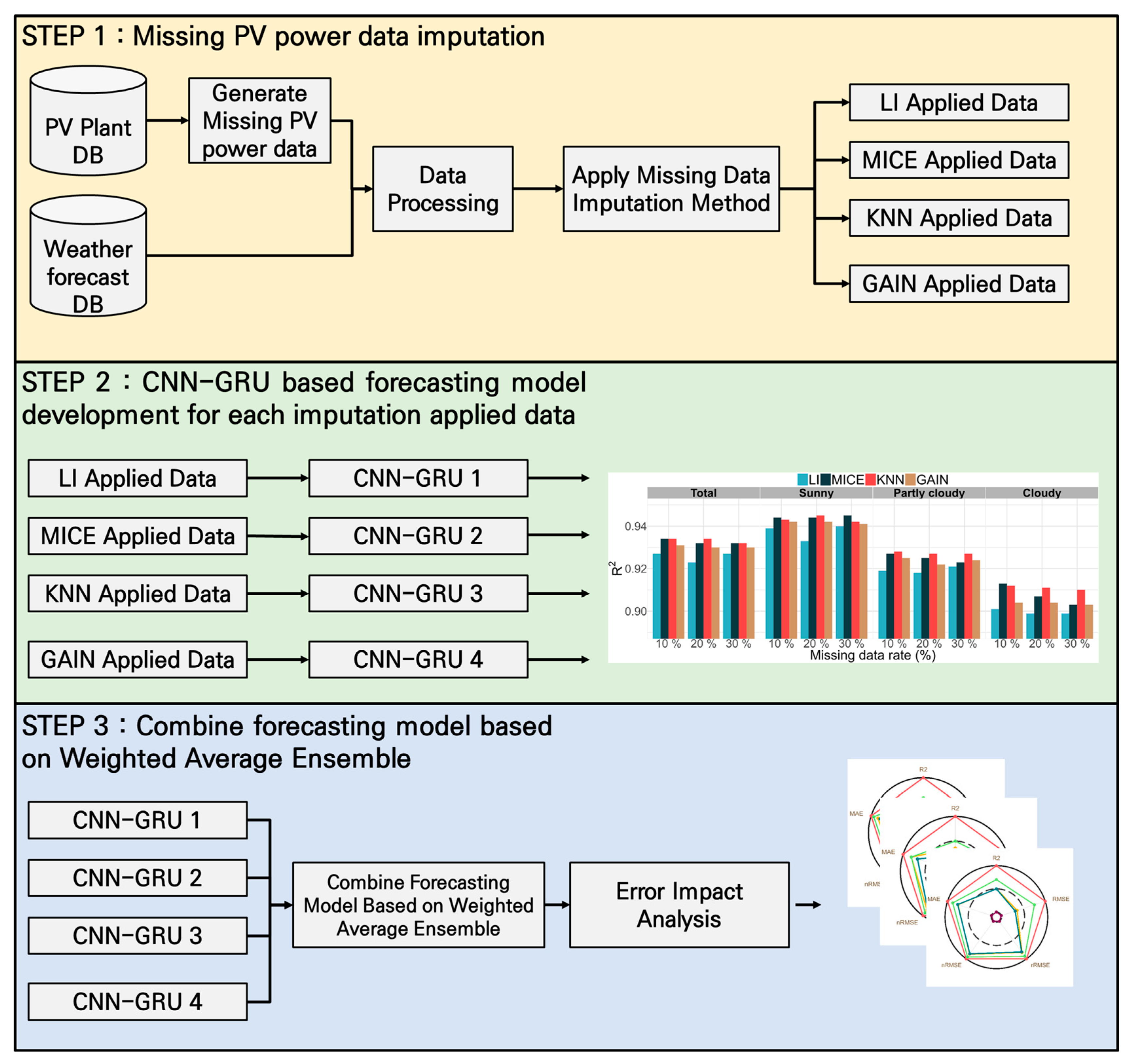
2. Methods
2.1. Imputation Methods
2.2. Forecasting Methods
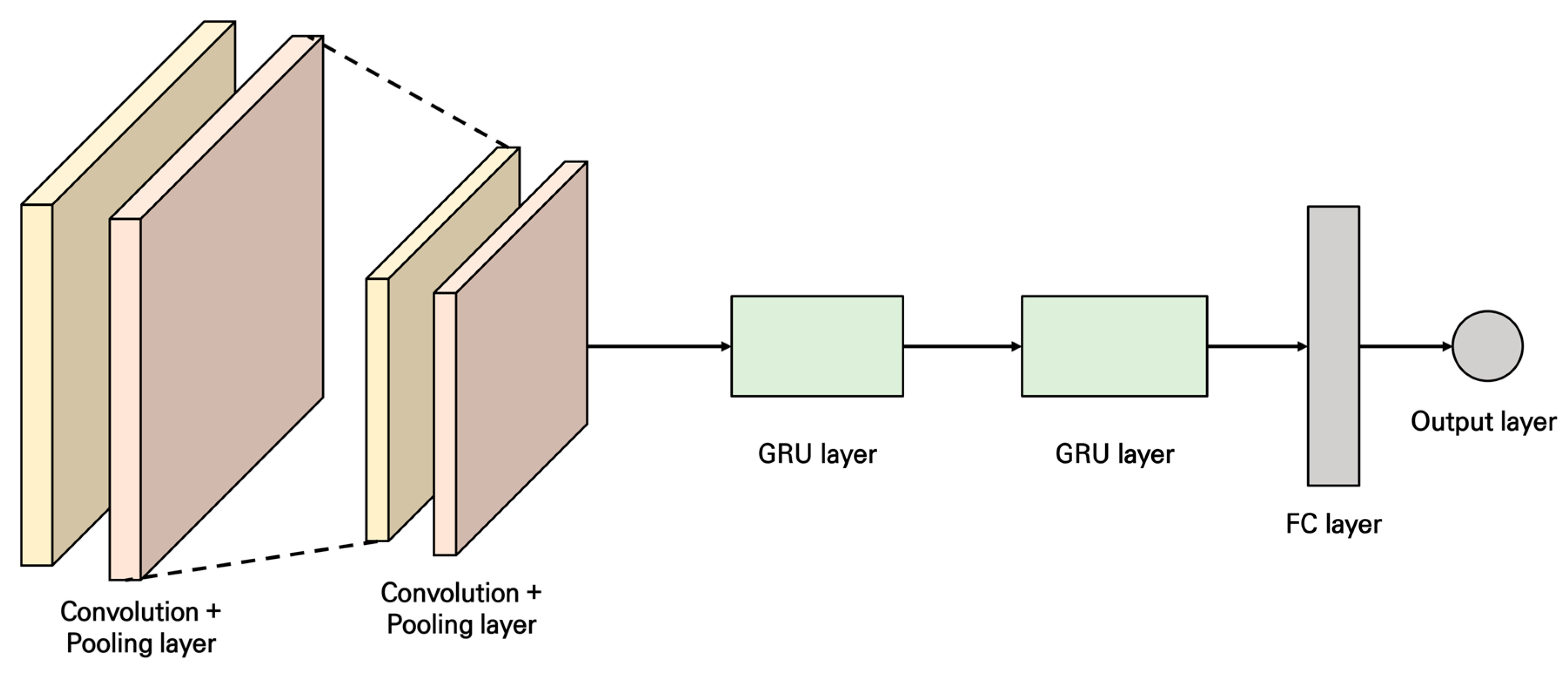
2.2.1. CNN-GRU
2.2.2. Weighted Average Ensemble
2.3. Performance Evaluation Index
3. Imputation of Missing PV Power Data
3.1. Data Description
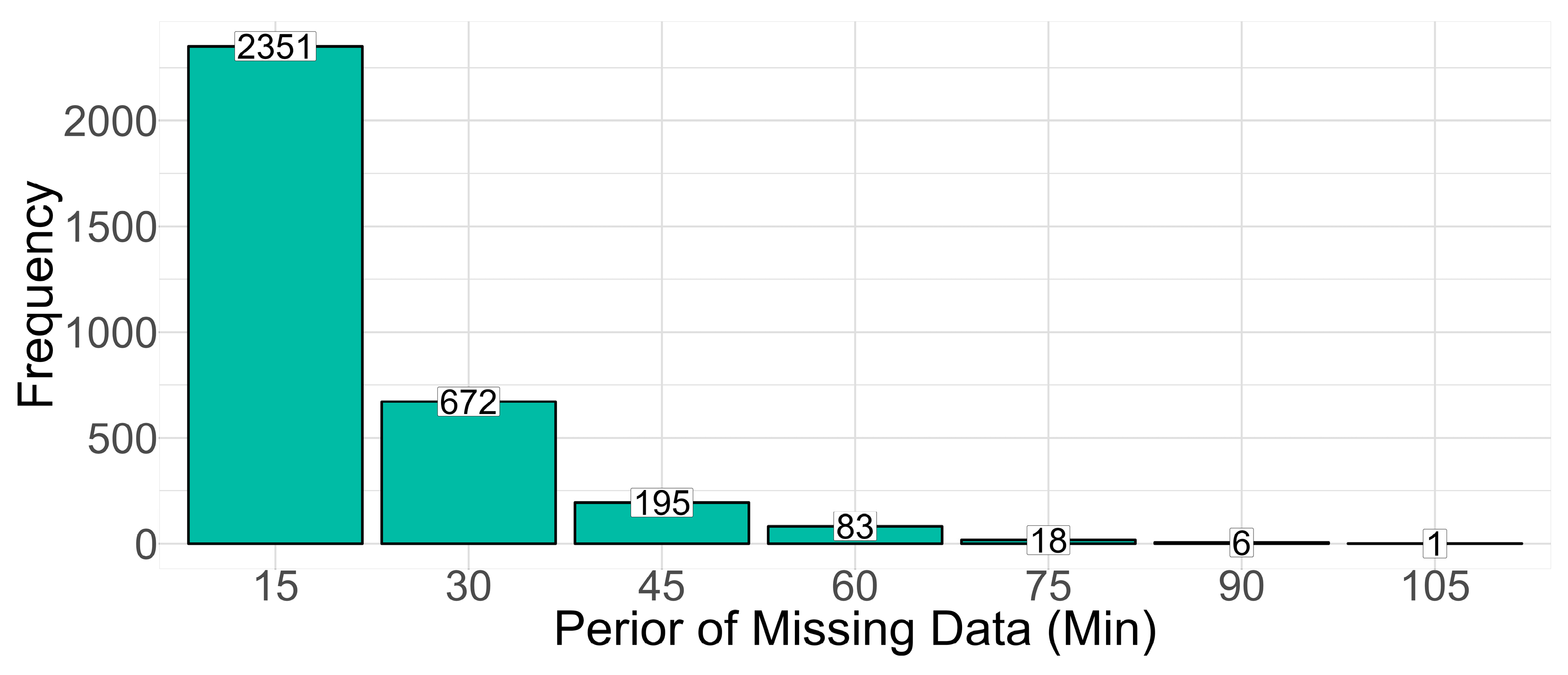
3.2. Generate Missing PV Power Data
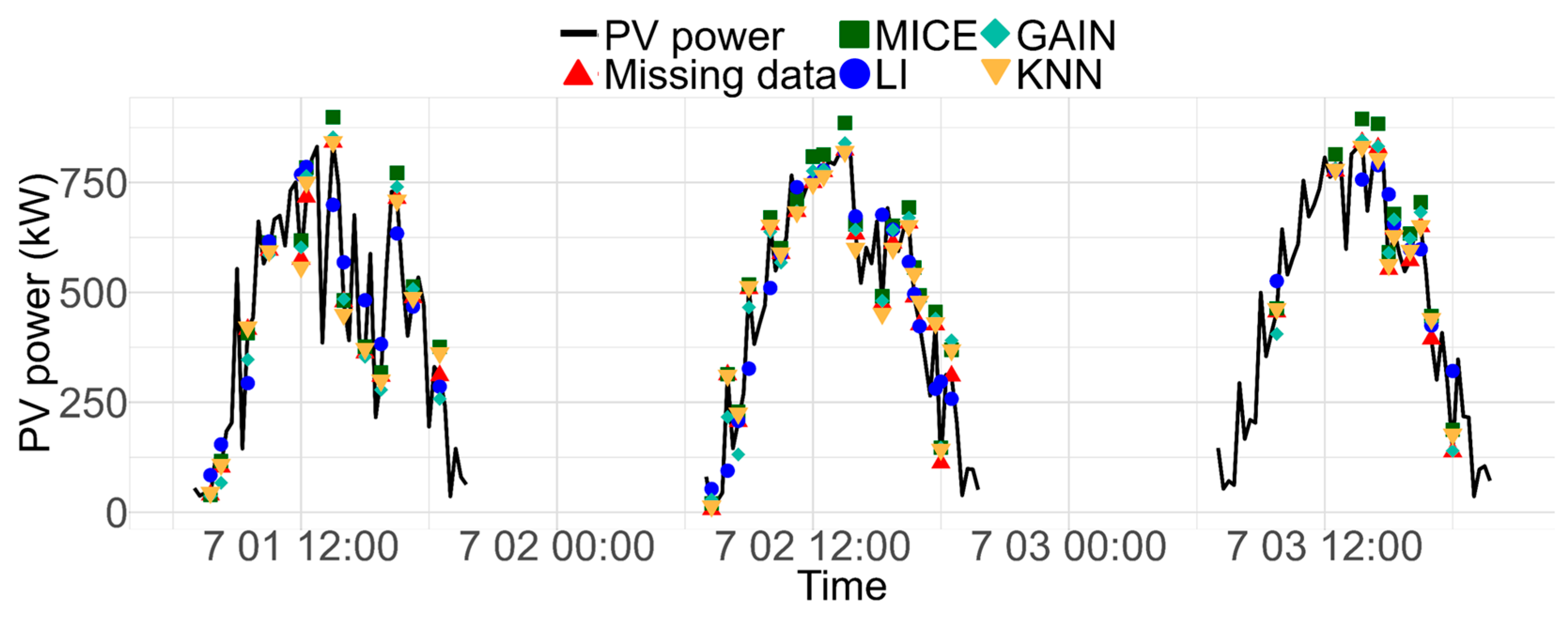
3.3. Impute Missing PV Power Data
4. Developing a PV Forecasting Model Using Imputation Method Applied Data
4.1. Developed a PV Power Forecasting Model Applying a Single Imputation
4.2. Combine PV Forecasting Model Based on Weighted Average Ensemble
5. Conclusions
Author Contributions
Funding
Institutional Review Board Statement
Informed Consent Statement
Data Availability Statement
Acknowledgments
Conflicts of Interest
References
- IRENA. Renewable Capacity Statistics 2024. Available online: https://www.irena.org/Publications/2024/Mar/Renewable-capacity-statistics-2024 (accessed on 9 April 2024).
- Iheanetu, K.J. Solar Photovoltaic Power Forecasting: A Review. Sustainability 2022, 14, 17005. [Google Scholar] [CrossRef]
- Akhter, M.N.; Mekhilef, S.; Mokhlis, H.; Almohaimeed, Z.M.; Muhammad, M.A.; Khairuddin, A.S.M.; Akram, R.; Hussain, M.M. An Hour-Ahead PV Power Forecasting Method Based on an RNN-LSTM Model for Three Different PV Plants. Energies 2022, 15, 2243. [Google Scholar] [CrossRef]
- Mohamad Radzi, P.N.L.; Akhter, M.N.; Mekhilef, S.; Mohamed Shah, N. Review on the Application of Photovoltaic Forecasting Using Machine Learning for Very Short-to Long-Term Forecasting. Sustainability 2023, 15, 2942. [Google Scholar] [CrossRef]
- Zhao, J.; Guo, Z.H.; Su, Z.Y.; Zhao, Z.Y.; Xiao, X.; Liu, F. An improved multi-step forecasting model based on WRF ensembles and creative fuzzy systems for wind speed. Appl. Energy 2016, 162, 808–826. [Google Scholar] [CrossRef]
- Lee, C.H.; Yang, H.C.; Ye, G.B. Predicting the performance of solar power generation using deep learning methods. Appl. Sci. 2021, 11, 6887. [Google Scholar] [CrossRef]
- Udawalpola, R.; Masuta, T.; Yoshioka, T.; Takahashi, K.; Ohtake, H. Reduction of power imbalances using battery energy storage system in a bulk power system with extremely large photovoltaics interactions. Energies 2021, 14, 522. [Google Scholar] [CrossRef]
- Wang, X.; Hyndman, R.J.; Li, F.; Kang, Y. Forecast combinations: An over 50-year review. Int. J. Forecast. 2023, 39, 1518–1547. [Google Scholar] [CrossRef]
- Akhter, M.N.; Mekhilef, S.; Mokhlis, H.; Ali, R.; Usama, M.; Muhammad, M.A.; Khairuddin, A.S.M. A hybrid deep learning method for an hour ahead power output forecasting of three different photovoltaic systems. Appl. Energy 2022, 307, 118185. [Google Scholar] [CrossRef]
- Lateko, A.A.; Yang, H.T.; Huang, C.M. Short-term PV power forecasting using a regression-based ensemble method. Energies 2022, 15, 4171. [Google Scholar] [CrossRef]
- AlKandari, M.; Ahmad, I. Solar power generation forecasting using ensemble approach based on deep learning and statistical methods. Appl. Comput. Inform. 2020. [Google Scholar] [CrossRef]
- Banik, R.; Biswas, A. Improving Solar PV Prediction Performance with RF-CatBoost Ensemble: A Robust and Complementary Approach. Renew. Energy Focus 2023, 46, 207–221. [Google Scholar] [CrossRef]
- Sharma, N.; Mangla, M.; Yadav, S.; Goyal, N.; Singh, A.; Verma, S.; Saber, T. A sequential ensemble model for photovoltaic power forecasting. Comput. Electr. Eng. 2021, 96, 107484. [Google Scholar] [CrossRef]
- Choi, J.; Lee, I.W.; Cha, S.W. Analysis of data errors in the solar photovoltaic monitoring system database: An overview of nationwide power plants in Korea. Renew. Sustain. Energy Rev. 2022, 156, 112007. [Google Scholar] [CrossRef]
- Zhang, W.; Luo, Y.; Zhang, Y.; Srinivasan, D. SolarGAN: Multivariate solar data imputation using generative adversarial network. IEEE Trans. Sustain. Energy 2020, 12, 743–746. [Google Scholar] [CrossRef]
- Park, S.; Park, S.; Kim, M.; Hwang, E. Clustering-based self-imputation of unlabeled fault data in a fleet of photovoltaic generation systems. Energies 2020, 13, 737. [Google Scholar] [CrossRef]
- Fan, Y.; Yu, X.; Wieser, R.; Meakin, D.; Shaton, A.; Jaubert, J.N.; Flottemesch, R.; Howell, M.; Braid, J.; Bruckman, L.S.; et al. Spatio-Temporal Denoising Graph Autoencoders with Data Augmentation for Photovoltaic Timeseries Data Imputation. arXiv 2023, arXiv:2302.10860. [Google Scholar]
- de-Paz-Centeno, I.; García-Ordás, M.T.; García-Olalla, Ó.; Alaiz-Moretón, H. Imputation of missing measurements in PV production data within constrained environments. Expert Syst. Appl. 2023, 217, 119510. [Google Scholar] [CrossRef]
- Lindig, S.; Louwen, A.; Moser, D.; Topic, M. Outdoor PV system monitoring—Input data quality, data imputation and filtering approaches. Energies 2020, 13, 5099. [Google Scholar] [CrossRef]
- Kang, M.; Zhu, R.; Chen, D.; Liu, X.; Yu, W. CM-GAN: A Cross-Modal Generative Adversarial Network for Imputing Completely Missing Data in Digital Industry. IEEE Trans. Neural Netw. Learn. Syst. 2023. [CrossRef]
- Liu, X.; Huang, C.; Wang, L.; Luo, X. Improved super-resolution perception convolutional neural network for photovoltaics missing data recovery. Energy Rep. 2023, 9, 388–395. [Google Scholar] [CrossRef]
- Bülte, C.; Kleinebrahm, M.; Yilmaz, H.Ü.; Gómez-Romero, J. Multivariate time series imputation for energy data using neural networks. Energy AI 2023, 13, 100239. [Google Scholar] [CrossRef]
- Guo, G.; Zhang, M.; Gong, Y.; Xu, Q. Safe multi-agent deep reinforcement learning for real-time decentralized control of inverter based renewable energy resources considering communication delay. Appl. Energy 2023, 349, 121648. [Google Scholar] [CrossRef]
- Shireen, T.; Shao, C.; Wang, H.; Li, J.; Zhang, X.; Li, M. Iterative multi-task learning for time-series modeling of solar panel PV outputs. Appl. Energy 2018, 212, 654–662. [Google Scholar] [CrossRef]
- Kim, T.; Ko, W.; Kim, J. Analysis and impact evaluation of missing data imputation in day-ahead PV generation forecasting. Appl. Sci. 2019, 9, 204. [Google Scholar] [CrossRef]
- Girimurugan, R.; Selvaraju, P.; Jeevanandam, P.; Vadivukarassi, M.; Subhashini, S.; Selvam, N.; Hasane, A.S.K.; Mayakannan, S.; Vaithilingam, S.K. Application of Deep Learning to the Prediction of Solar Irradiance through Missing Data. Int. J. Photoenergy 2023, 2023, 4717110. [Google Scholar] [CrossRef]
- Lee, D.S.; Lai, C.W.; Fu, S.K. A Short-and Medium-Term Forecasting Model for Roof PV Systems with Data Pre-Processing. Heliyon 2024, 10, e27752. [Google Scholar] [CrossRef] [PubMed]
- Lee, D.S.; Son, S.Y. PV forecasting model development and impact assessment via imputation of missing PV power data. IEEE Access 2024, 12, 12843–12852. [Google Scholar] [CrossRef]
- Zhang, Y.; Zhang, R.; Zhao, B. A systematic review of generative adversarial imputation network in missing data imputation. Neural Comput. Appl. 2023, 35, 19685–19705. [Google Scholar] [CrossRef]
- Zhang, Y.; Thorburn, P.J. Handling missing data in near real-time environmental monitoring: A system and a review of selected methods. Future Gener. Comput. Syst. 2022, 128, 63–72. [Google Scholar] [CrossRef]
- Aleryani, A.; Bostrom, A.; Wang, W.; Iglesia, B. Multiple Imputation Ensembles for Time Series (MIE-TS). ACM Trans. Knowl. Discov. Data 2023, 17, 1–28. [Google Scholar] [CrossRef]
- Azur, M.J.; Stuart, E.A.; Frangakis, C.; Leaf, P.J. Multiple imputation by chained equations: What is it and how does it work? Int. J. Methods Psychiatr. Res. 2011, 20, 40–49. [Google Scholar] [CrossRef] [PubMed]
- Žliobaitė, I.; Hollmén, J. Optimizing regression models for data streams with missing values. Mach. Learn. 2015, 99, 47–73. [Google Scholar] [CrossRef]
- Chiu, M.C.; Hsu, H.W.; Chen, K.S.; Wen, C.Y. A hybrid CNN-GRU based probabilistic model for load forecasting from individual household to commercial building. Energy Rep. 2023, 9, 94–105. [Google Scholar] [CrossRef]
- Tovar, M.; Robles, M.; Rashid, F. PV power prediction, using CNN-LSTM hybrid neural network model. Case of study: Temixco-Morelos, México. Energies 2020, 13, 6512. [Google Scholar] [CrossRef]
- Alhussein, M.; Aurangzeb, K.; Haider, S.I. Hybrid CNN-LSTM model for short-term individual household load forecasting. IEEE Access 2020, 8, 180544–180557. [Google Scholar] [CrossRef]
- Sajjad, M.; Khan, Z.A.; Ullah, A.; Hussain, T.; Ullah, W.; Lee, M.Y.; Baik, S.W. A novel CNN-GRU-based hybrid approach for short-term residential load forecasting. IEEE Access 2020, 8, 143759–143768. [Google Scholar] [CrossRef]
- Lynn, H.M.; Pan, S.B.; Kim, P. A deep bidirectional GRU network model for biometric electrocardiogram classification based on recurrent neural networks. IEEE Access 2019, 7, 145395–145405. [Google Scholar] [CrossRef]
- Kumar, V.; Aydav, P.S.S.; Minz, S. Multi-view ensemble learning using multi-objective particle swarm optimization for high dimensional data classification. J. King Saud Univ.-Comput. Inf. Sci. 2022, 34, 8523–8537. [Google Scholar] [CrossRef]
- Anand, V.; Gupta, S.; Gupta, D.; Gulzar, Y.; Xin, Q.; Juneja, S.; Shah, A.; Shaikh, A. Weighted average ensemble deep learning model for stratification of brain tumor in MRI images. Diagnostics 2023, 13, 1320. [Google Scholar] [CrossRef]
- Shahhosseini, M.; Hu, G.; Pham, H. Optimizing ensemble weights and hyperparameters of machine learning models for regression problems. Mach. Learn. Appl. 2022, 7, 100251. [Google Scholar] [CrossRef]
- Baradaran, R.; Amirkhani, H. Zero-shot estimation of base models’ weights in ensemble of machine reading comprehension systems for robust generalization. In Proceedings of the 26th International Computer Conference, Computer Society of Iran (CSICC), Tehran, Iran, 3–4 March 2021; pp. 1–5. [Google Scholar]
- Diebold, F.X.; Mariano, R.S. Comparing predictive accuracy. J. Bus. Econ. Stat. 1995, 13, 253–263. [Google Scholar] [CrossRef]


| Imputation Method | Missing Data Rate (%) | Sky Status | |||
|---|---|---|---|---|---|
| Total | Sunny | Partly Cloudy | Cloudy | ||
| LI | 10 | 0.871 | 0.892 | 0.853 | 0.818 |
| 20 | 0.866 | 0.881 | 0.857 | 0.826 | |
| 30 | 0.865 | 0.878 | 0.861 | 0.816 | |
| MICE | 10 | 0.976 | 0.969 | 0.981 | 0.980 |
| 20 | 0.972 | 0.969 | 0.971 | 0.970 | |
| 30 | 0.967 | 0.961 | 0.965 | 0.972 | |
| KNN | 10 | 0.975 | 0.962 | 0.977 | 0.985 |
| 20 | 0.977 | 0.967 | 0.979 | 0.987 | |
| 30 | 0.976 | 0.967 | 0.977 | 0.987 | |
| GAIN | 10 | 0.924 | 0.917 | 0.942 | 0.927 |
| 20 | 0.916 | 0.922 | 0.922 | 0.908 | |
| 30 | 0.941 | 0.939 | 0.944 | 0.935 | |
| Missing Data Rate (%) | Imputation Method | |||
|---|---|---|---|---|
| LI | MICE | KNN | GAIN | |
| 10 | 0.02 | 1.13 | 0.03 | 30.88 |
| 20 | 0.01 | 1.40 | 0.03 | 23.76 |
| 30 | 0.02 | 0.94 | 0.04 | 25.30 |
| Average | 0.02 | 1.16 | 0.03 | 26.65 |
| Proposed Model | ||
|---|---|---|
| Conv1D | Filters | 32 |
| Activation | ELU | |
| Conv1D | Filters | 64 |
| Activation | ELU | |
| Conv1D | Filters | 128 |
| Activation | ELU | |
| Conv1D | Filters | 256 |
| Activation | ELU | |
| GRU | Hidden node | 128 |
| Activation | ELU | |
| GRU | Hidden node | 64 |
| Activation | ELU | |
| Output | Hidden node | 1 |
| Activation | ELU | |
| Missing Data Rate (%) | Model 1 | Model 2 | p-Value |
|---|---|---|---|
| 10 | Proposed | Ensemble | 0.001 |
| 20 | Proposed | Ensemble | 0.778 |
| 30 | Proposed | Ensemble | 0.003 |
| Index | Sunny | Partly Cloudy | Cloudy | Preferred Method | ||||||
|---|---|---|---|---|---|---|---|---|---|---|
| Missing Data Rate | 10% | 20% | 30% | 10% | 20% | 30% | 10% | 20% | 30% | |
| R2 | Proposed | Proposed | Proposed | Proposed | Proposed | Proposed | Proposed | Proposed | Proposed | Proposed |
| RMSE | Proposed | Proposed | Proposed | Proposed | Proposed | Proposed | Proposed | Proposed | Proposed | Proposed |
| rRMSE | Proposed | Proposed | Proposed | Proposed | Proposed | Proposed | Proposed | Proposed | Proposed | Proposed |
| nRMSE | Proposed | Proposed | Proposed | Proposed | Proposed | Proposed | Proposed | Proposed | Proposed | Proposed |
| MAE | Proposed | Proposed | Proposed | Proposed | Proposed | Proposed | Proposed | Proposed | Proposed | Proposed |
| Preferred method | Proposed | Proposed | Proposed | Proposed | Proposed | Proposed | Proposed | Proposed | Proposed | Proposed |
Disclaimer/Publisher’s Note: The statements, opinions and data contained in all publications are solely those of the individual author(s) and contributor(s) and not of MDPI and/or the editor(s). MDPI and/or the editor(s) disclaim responsibility for any injury to people or property resulting from any ideas, methods, instructions or products referred to in the content. |
© 2024 by the authors. Licensee MDPI, Basel, Switzerland. This article is an open access article distributed under the terms and conditions of the Creative Commons Attribution (CC BY) license (https://creativecommons.org/licenses/by/4.0/).
Share and Cite
Lee, D.-S.; Son, S.-Y. Weighted Average Ensemble-Based PV Forecasting in a Limited Environment with Missing Data of PV Power. Sustainability 2024, 16, 4069. https://doi.org/10.3390/su16104069
Lee D-S, Son S-Y. Weighted Average Ensemble-Based PV Forecasting in a Limited Environment with Missing Data of PV Power. Sustainability. 2024; 16(10):4069. https://doi.org/10.3390/su16104069
Chicago/Turabian StyleLee, Dae-Sung, and Sung-Yong Son. 2024. "Weighted Average Ensemble-Based PV Forecasting in a Limited Environment with Missing Data of PV Power" Sustainability 16, no. 10: 4069. https://doi.org/10.3390/su16104069
APA StyleLee, D.-S., & Son, S.-Y. (2024). Weighted Average Ensemble-Based PV Forecasting in a Limited Environment with Missing Data of PV Power. Sustainability, 16(10), 4069. https://doi.org/10.3390/su16104069