1. Introduction
Engaging in physical activity during adolescence offers a range of advantages for physical, social, and psychological well-being [
1,
2,
3]. Therefore, the Centers for Disease Control and Prevention (CDC) advise that children and teenagers should participate in a minimum of 60 min of daily physical activity [
4]. However, studies indicate that only about one-third of children actually meet this recommendation. This concerning lack of sufficient physical activity among youth has become a prominent concern in the public health community [
5].
Consistent exercise is crucial for the physical and emotional health of children, particularly for those battling obesity. Children and adolescents who participate in physical activity are less likely to become overweight and obese during their youth and adolescence, and they are less likely to become obese as adults [
6,
7]. One potential factor that may contribute to increased physical activity and reduced childhood obesity is active commuting to school [
8,
9,
10,
11]. Surprisingly, when comparing data from 1969 to 2009, there has been a significant decline in the number of students who walk or cycle to school. In less than 40 years, the average of students walking or cycling to school has dropped from 42% to 13%. Statistics show that in 1969, 87% of those who lived within one mile of school would walk or bicycle to school, and this number decreased to almost half (47%) in 2009 [
12].
This paper centers on Chula Vista, San Diego County’s second-largest city, which houses a significant number of school-aged children. With approximately 270,000 residents, a quarter of whom are children under the age of eighteen, the city has around fifty-two elementary schools. Alarmingly, 38% of school-aged children in Chula Vista were reported as overweight/obese by 2010 [
13]. Highlighting the city’s challenges, the Social Vulnerability Index (SVI) from the Centers for Disease Control and Prevention (CDC) and the Agency for Toxic Substances and Disease Registry (ATSDR) ranks Chula Vista among the cities with the highest social vulnerability in San Diego County [
14]. This vulnerability is gauged through various metrics such as poverty and vehicle access, among others.
In an effort to promote Active Transportation to School (ATS), the Safe Routes to School (SRTS) program was introduced. SRTS is a federally funded program which encourages students to walk and cycle to school through 6 Es: engagement, equity, engineering, encouragement, education, and evaluation. This program focuses on both infrastructure improvements and educational programs and hopes to foster a culture of active transportation among students. Since 2005, more than 14,000 schools all across the US have participated in this program [
15]. The Chula Vista Elementary School District (CVESD) has been an active SRTS participant since 2007. Numerous activities and projects were initiated by SRTS in CVESD, including pedestrian safety educational programs and bicycle rodeos.
Surveys have proven to be a valuable and cost-effective method for collecting information from a large population [
16]. Consequently, the National Center for Safe Routes to School program has provided standardized surveys, including the Parent survey, which seeks information about students’ modes of transport, factors influencing parental decisions regarding their child’s commute, safety conditions along routes to school, and other relevant background information. These surveys can play a crucial role in identifying barriers to active transportation and measuring changes in parental attitudes as a result of local SRTS programs. To evaluate the effectiveness of SRTS programs on active transportation trends among CVESD students, responses to the Parent survey were collected before, during, and after the implementation of SRTS activities.
This research aims to explore the factors that hinder students from engaging in Active Transportation to School, with a particular focus on understanding the perspectives of parents, the role of schools in promoting active transportation, and the influence of students’ home distance from school. By thoroughly investigating these barriers, we aspire to uncover valuable insights that can pave the way for effective interventions and initiatives to encourage active transportation among students.
Furthermore, this study seeks to assess the impact of the SRTS activities on the promotion of active transportation. We rigorously analyzed whether the implementation of SRTS initiatives leads to a significant increase in the percentage of students utilizing active modes of transportation, such as walking or cycling, to commute to school. By examining data from various stages of the program, including pre-implementation, mid-implementation, and post-implementation, this study provides a comprehensive understanding of the program’s effectiveness over time.
Following an extensive literature review on the subject matter, the authors of this study utilized multiple machine learning algorithms. Leveraging data collected by the National Center for Safe Routes to School, we employed advanced statistical techniques and predictive modeling to pinpoint key factors that influence students’ transportation choices.
The findings of this research have the potential to generate promising outcomes and inform evidence-based strategies to overcome barriers to active transportation among students. By thoroughly analyzing the Parent survey, we can develop targeted interventions that promote and sustain active transportation behaviors. Ultimately, this study contributes to the development of practical and impactful approaches that will empower more students to embrace active transportation and lead healthier, more active lives.
2. Previous Work
Many of the previous studies on the Safe Routes to School primarily focus on changes in travel behavior associated with SRTS program interventions. These studies have predominantly highlighted the impact of infrastructure improvements on ATS [
17,
18,
19]. While there may be a positive correlation between traffic improvements and an increase in ATS rates, it should be noted that infrastructure enhancements alone might not be sufficient to promote cycling and walking in schools with low levels of activity [
20]. In fact, previous research suggests that non-infrastructure measures, such as educational programs, can effectively encourage walking and biking to school [
21,
22,
23].
In addition to infrastructural and non-infrastructural factors, there are several elements that influence the likelihood of engaging in active modes of transportation when traveling to and from school. Previous research has emphasized the significance of home-to-school distance in determining the rate of active transportation among children and adolescents [
24,
25]. Notably, a greater home-to-school distance between the residential area and the school has been identified as a robust predictor of active transportation behavior in children and adolescents [
26,
27,
28]. Increased distances between home and school often result in children traveling on arterial roads and having to cross them, which poses significant traffic-related safety challenges [
29]. Recent studies have demonstrated that parents’ attitudes toward Active Transportation to School have become more negative as the distance between their homes and schools has increased [
30].
In addition to the home-to-school distance, mediating factors can also influence students’ decision to use ATS [
31]. These mediating factors encompass the direct influence of the social and natural environment, such as crime rates and traffic collision rates, as well as the perceptual interpretations of parents and children regarding their surroundings, including perceived risks associated with crime or traffic. In some locales, regional policies and land development also significantly shape these active transportation choices [
32]. A thorough examination of over 60 papers on active travel has revealed the impact of mediating factors such as age and education levels in travel preferences. Some of the previous studies suggest that active travel decreases with age, with men and those with higher education preferring biking, while women tend to choose walking. Moreover, these studies consistently note lower bike usage among minorities and those with lower incomes [
33].
Previous research by Davison et al. suggests that parental perceptions of the environment have a stronger impact on transportation patterns to school than built environment factors alone [
11]. Parents’ concerns about traffic and safety related to ATS are significant factors contributing to the increasing number of parents choosing to drive their children to and from school [
8,
34]. Previous studies indicate that parental barriers to engaging in active commuting are shaped by various factors, including the age, gender, mode of transportation employed by their children [
35], and parents’ level of education [
36,
37,
38]. Parents’ concerns primarily arise from the absence of sidewalks, the presence of heavy traffic, high-speed roads, risky pedestrian crossings, and personal safety issues such as crime, collectively shaping their perception of unsafe routes to school [
39,
40,
41,
42]. The concerns of parents regarding traffic, crime, and personal safety can significantly influence the choice of transportation mode to school for adolescents, consequently shaping their perceptions of the route and their behavior regarding Active Transportation to School [
30,
43,
44]. Specifically, personal safety concerns, such as local crime rates and the presence of strangers in the neighborhood, also discourage children from engaging in ATS and opting to walk or cycle to school [
45,
46]. Moreover, parental concerns about the safety of their children while walking and cycling to school are further compounded by the lack of adult supervision [
47,
48].
Barriers to active transportation can have a significant impact on participation rates. Studies have shown that children who do not face reported barriers are more likely to walk or bike to school compared to their peers who encounter one or more barriers [
49]. Therefore, it is crucial to address traffic and personal safety concerns when developing models for safe walking and cycling routes to schools [
50]. By considering these findings, efforts can be made to create frameworks that address these barriers, ultimately promoting and encouraging active transportation among children and adolescents. By addressing these barriers, we can further enhance our understanding of the factors influencing active transportation to school and develop evidence-based strategies that promote safe and sustainable travel options for children and adolescents. Such efforts can contribute to creating healthier, more livable communities where Active Transportation to School becomes the norm rather than the exception.
In the landscape of school travel mode choice modeling, logistic regression (LR) has remained a time-tested and trusted tool. Numerous studies have explored its capabilities; for instance, a study spanning from 2007 to 2018 in Arizona employed LR to identify students’ chosen modes of transport to school [
51]. Another notable investigation utilized it to evaluate the challenges faced by student commuters, considering diverse demographic and institutional factors [
52]. Such varied applications underscore LR’s essential role in educational inquiries. Moving into more recent analytical advancements, the random forest (RF) technique is gaining ground in transportation studies. Previous work [
53,
54,
55] serves as proof of RF’s capability to navigate and interpret complex traveler behaviors. Further solidifying its value, one previous study’s [
56] exploration using RF on Nanjing’s travel diary data emphasized the method’s strength in both enhancing prediction accuracy and analyzing travel determinants. Lastly, support vector machines (SVM) have also demonstrated significant efficacy in this field. Dave et al.’s study on the transportation preferences of Vadodara’s schoolchildren and Assi, Khaled J., et al.’s innovative blend of SVM with clustering techniques to forecast student travel mode decisions highlight SVM’ pivotal importance [
57,
58]. Together, LR, RF, and SVM offer a comprehensive analytical framework, each contributing uniquely to our understanding and prediction of school travel mode choices.
Given the SRTS initiatives in Chula Vista, a prior study examined students’ transportation habits and underscored the importance of factors such as school proximity, crime concerns, and school encouragement in shaping student decisions [
59]. Building on this research, the current study aims to extend the existing literature by conducting an analysis of survey data gathered from parents at distinct stages—pre-implementation, mid-implementation, and post-implementation—of these active transportation initiatives. With this approach, we seek to provide a deeper understanding of evolving parental concerns and perceptions as these interventions unfold over time.
3. Methodology
3.1. Data Collection
The surveys created by the National Center for Safe Routes to School were studied to provide a better insight into the school travel environment. The Parent survey proposed by this center gathers information from parents/guardians on their children’s travel behavior, including their usual transportation mode and how far they live from their school, and the concerns parents may have for active transportation. This survey mainly focuses on the issues that may affect parents’ willingness or permission for their children to walk/bicycle to school. The Parent survey also includes children’s background information (age, gender), and if parents are concerned about twelve potential issues mentioned in the survey. This can be used as a powerful tool to investigate the underlying reasons why students are (or are not) considering active school travel, and if these issues arise from safety concerns or parents’ perceptions. The Parent dataset used in this research was gathered and consolidated for all SRTS participant schools in CVESD, and included 5764 surveys collected from 19 schools between 2009 and 2011, for students aged from Pre-K to sixth grade.
Table 1 presents a detailed overview of the features derived from the Parent Survey, along with their respective explanations.
According to the American Academy of Pediatrics (AAP) [
60] and previous studies [
61,
62], it is generally recommended that children wait until they are in fifth grade, around the age of 10, before walking to school without adult supervision. Hence, this study only focused on the data from 5th to 12th grade students. After removing the irrelevant student age groups (Pre-K to fourth grade) and some missing values, the data were reduced to 1387 observations.
3.2. Statistical Analysis
The primary objective of this research was to investigate the factors influencing the choice of transportation mode for students traveling to school, focusing on active transportation. Due to the limited number of observations for bicycling, the analysis was narrowed down to solely examine walking. However, it should be noted that the same analytical framework can be readily applied to bicycling data if a sufficient volume of observations becomes available.
We extracted independent variables from the Parent survey and used them alongside transportation mode as the dependent variable in our analysis. Transportation mode indicated in the Parent survey was transformed into a binary classification format, indicating whether the student walks as their usual commuting mode (Transportation Mode = 1) or if they use any other transportation mode (Transportation Mode = 0).
The independent variables used in the analysis encompassed factors such as students’ gender, distance between home and school, the role of the school in promoting active transportation, as well as parents’ education level, perceptions, and concerns regarding active transportation.
To identify the key factors influencing the decision to walk to school, we employed multiple machine learning algorithms, namely logistic regression (LR), random forest (RF), and support vector machines (SVM). Given the potential issue of multicollinearity arising from highly correlated independent variables [
63,
64], we performed a preliminary analysis to identify and remove such variables. Additionally, to mitigate overfitting concerns and obtain more accurate estimates, we applied 5-fold cross-validation to each model [
65,
66]. Finally, SHapley Additive exPlanations values (SHAP) were used as a means of feature selection and compared across the models to identify the most significant factors influencing the prevalence of walking to school.
It is worth noting that the Parent survey provided options for two transportation modes: morning (going to school) and evening (coming back home). One of the objectives of this research was to compare these responses and determine if significant differences existed in the patterns of walking to and from school. Accordingly, two logistic regression models were constructed for this comparison. The results did not show significant variations, with a slightly higher prevalence of students walking back home in the evening (27%) compared to walking to school in the morning (23%). Consequently, this paper only used the morning transportation mode as the response variable in all three models.
3.3. Model Selection
3.3.1. Logistic Regression
Regression methods have emerged as a fundamental component of data analysis in exploring the connection between a dependent variable and one or multiple independent variables. Logistic regression, a statistical model commonly employed in traffic safety studies [
67,
68,
69,
70,
71], has been utilized for investigating the association between a binary response variable and independent variables.
Logistic regression is a powerful statistical tool optimized for predicting binary outcomes based on one or more explanatory variables. Unlike linear regression, which predicts continuous values, logistic regression focuses on estimating the probability that a given observation falls into a specific category. Central to this method is the logistic function, which constrains predicted probabilities to lie between 0 and 1 [
72].
Mathematically, for predictor variables denoted as
X1,
X2, …
Xn, the probability of the desired outcome is modeled as:
In this formulation, the term P(X) indicates the likelihood of the event in question. The coefficients (β0, β1, … βn) represent the influence of each predictor variable on the log odds of the outcome. Specifically, a coefficient reveals how the log odds of the outcome change with a one-unit increase in its associated predictor, while keeping all other predictors constant. The values of these coefficients are determined using the Maximum Likelihood Estimation (MLE) method. This method aims to find the coefficient values that are most likely to produce the observed data, given the model’s structure.
3.3.2. Random Forest
Random forest (RF) is an ensemble model that effectively leverages decision trees to handle complex, nonlinear relationships and high-dimensional variables, while exhibiting robustness against outliers and noise [
73]. The essence of RF lies in its bootstrapping technique and aggregation method. For each tree, a subset of data is sampled with replacement (bootstrap sample), and a subset of features is chosen randomly to split the nodes. This diversification ensures that individual trees capture different patterns in the data. The final prediction, for classification, is based on a majority vote, and for regression, it is the average of the predictions from all trees [
72]. Given its capabilities, RF has garnered considerable recognition and has been widely applied in various transportation research contexts [
74,
75,
76,
77,
78].
For a classification problem, given a new observation
X, the
RF prediction is:
where
is the prediction of the
ith tree. For regression, it is the average:
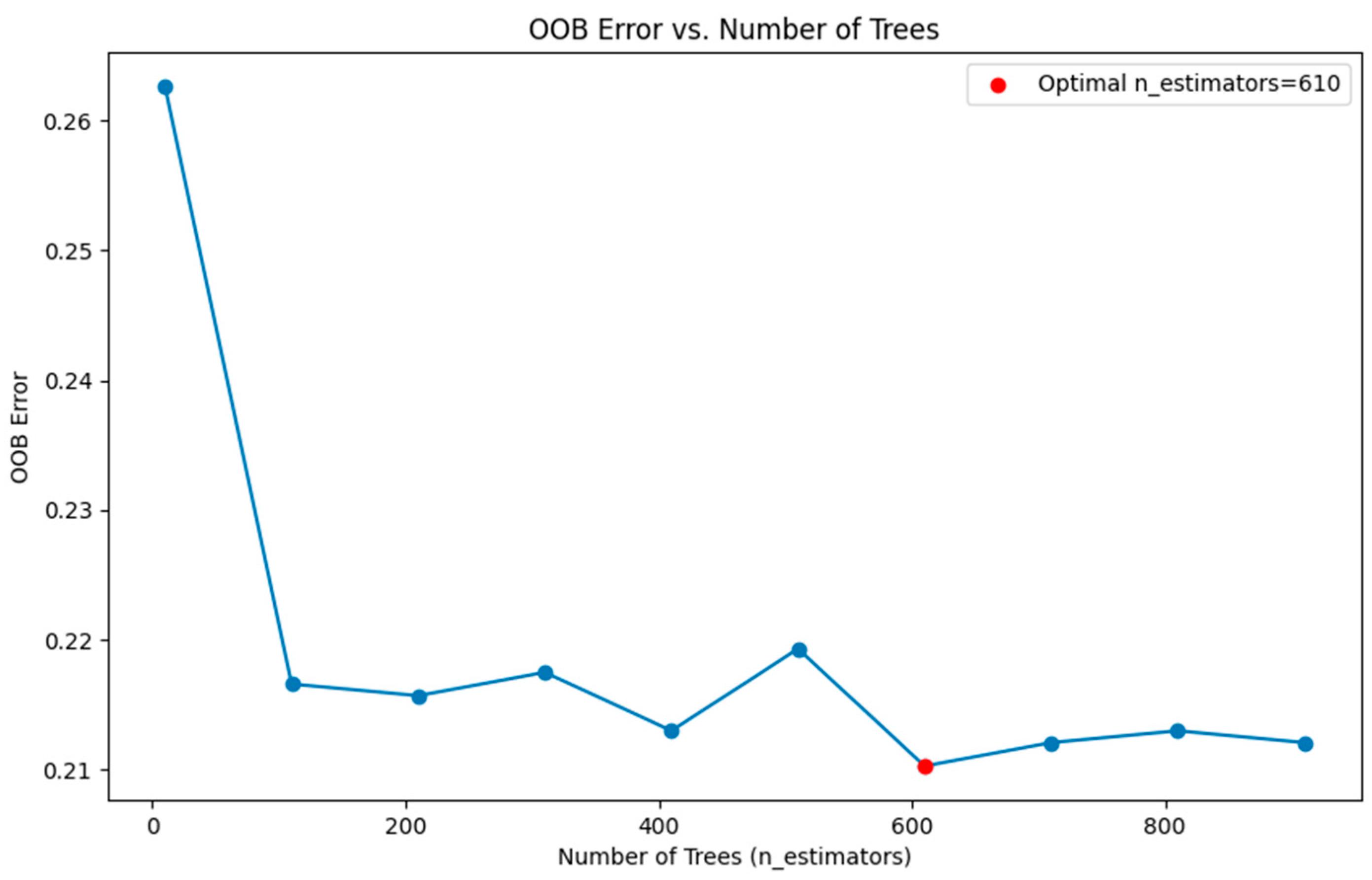
The efficacy of random forest (RF) models is substantially impacted by the configuration of hyperparameters. To maximize the performance of RF, it is imperative to identify the most suitable parameter values through careful optimization. By emphasizing the objective of minimizing the out-of-bag (OOB) error and identifying the optimal number of trees for the RF model, the development of the optimal random forest model was accomplished following a 5-fold cross-validation procedure.
3.3.3. Support Vector Machines
Support vector machines (SVM) are widely recognized as one of the highly effective algorithms for classification and regression problems. Due to their extensive application and reliable performance across various scientific domains, SVM have been a focal point in transportation research in recent years [
79,
80,
81]. One prominent application of this model is for binary classification tasks, aiming to identify the optimal hyperplane that effectively partitions the data into two distinct classes [
82,
83].
SVM aim to find a hyperplane defined by
w (weight vector) and
b (bias) that maximizes the margin between two classes. This margin represents the distance between the hyperplane and the nearest data points, or “support vectors”, from both classes. Given labeled data
where
, the decision function is defined as:
The primary goal is to optimize:
Here, the objective is to strike a balance. The term seeks the hyperplane with the largest possible margin, while allows for some flexibility, permitting certain points to be on the “wrong side” of the hyperplane for the sake of better overall fit. The parameter “C” determines this balance: higher values stress the importance of each data point being correctly classified, even if it means a smaller margin.
The SVM model was developed using scikit-learn. In addition, the effectiveness of SVM can be substantially enhanced by employing parameter optimization techniques [
84,
85]. In this case, the grid search technique is employed to determine the best values for the regularization parameter “
C” and the radial basis kernel parameter “Gamma”. The grid search is performed within the context of a 5-fold cross-validation, ensuring reliable evaluation of the model’s performance.
3.4. Model Evaluation Metric
Accuracy and error rate are commonly used metrics for evaluating classification models in both binary and multi-class problems due to their simplicity, applicability to different scenarios, and ease of interpretation. However, these metrics have limitations in terms of producing less distinct and discriminative values and showing bias towards majority class instances [
86,
87]. To overcome these limitations, it is necessary to consider other evaluation metrics.
One widely used evaluation metric is the confusion matrix, which provides a comprehensive assessment of a classifier’s performance by capturing true positive, true negative, false positive, and false negative outcomes [
88]. The AUC (Area Under the ROC Curve) is another model evaluation metric for assessing classification model performance [
89,
90]. A value of 1 indicates an ideal model that can accurately separate positive and negative classes, while 0.5 indicates that it performs no better than random.
In this study, the evaluation of the proposed models included the assessment of AUC and confusion matrix, complementing the analysis based on accuracy and error rate. These diverse metrics provide a more comprehensive understanding of the model’s performance and contribute to a thorough evaluation process.
3.5. SHAP Values
SHapley Additive exPlanations, often referred to as SHAP, is a method used in machine learning to determine the impact of individual features on a model’s predictions [
91,
92]. By evaluating the contribution of each feature in the dataset to the overall output and considering all possible feature combinations, SHAP values provide insights into how different features affect the model’s predictions. Mathematically, the SHAP value of a feature
j for a specific instance
x can be expressed as:
where
N is the set of all features,
S is a subset of
N excluding feature
j, and
fx(
S) represents the model’s prediction when only features in subset
S are considered [
93]. This formula quantifies the marginal contribution of feature
j to the model’s prediction, averaged over all possible subsets of features, thereby providing an assessment of its pertinence relative to a baseline that takes into account all feature interactions.
This approach aids in understanding the contribution of each feature to the prediction result and can be used as a feature selection mechanism [
93,
94,
95]. In this study, SHAP values were utilized to determine and compare the most significant factors in ATS for each model. By comparing the SHAP values of each feature in the models, we identified the features that have the most substantial impact on the prediction outcomes.
In binary classification, SHAP values generally range between −1 and +1. These values represent a feature’s influence on the model’s output compared to the baseline prediction, often derived from the mean prediction of the dataset. A SHAP value in the positive domain suggests that a particular feature drives the model’s prediction toward the positive class, while a value in the negative domain indicates a push toward the negative class. The absolute magnitude of the SHAP value, irrespective of its sign, indicates the intensity of the feature’s effect on the model’s predictive outcome.
4. Results
As discussed earlier in the methodology section, the proposed machine learning models, namely logistic regression (LR), random forest (RF), and support vector machines (SVM), were employed to investigate the relationship between students’ transportation mode and various demographic and perceptual features extracted from the Parent survey. The objective was to predict the transportation mode using binary classification, with “walk” assigned a value of 1 and other transportation modes assigned a value of 0.
To enhance the performance of the models, hyperparameter tuning was conducted using Scikit Learn’s GridSearchCV method for LR and SVM, and RandomizedSearchCV for RF. GridSearchCV systematically explored a predefined grid of hyperparameter values, evaluating the effectiveness of the models through cross-validation. The optimal hyperparameter configuration was determined based on the highest performance score. RandomizedSearchCV, on the other hand, randomly sampled a subset of hyperparameter combinations from a specified distribution, reducing computational costs while still evaluating performance through cross-validation.
We opted for GridSearchCV for LR and SVM due to their relatively constrained hyperparameter tuning needs: LR is predominantly concerned with regularization aspects, while SVM concentrate on kernel choices. In contrast, RF presents a richer hyperparameter spectrum, encompassing decisions such as optimal tree count (
Figure 1), tree depth, and the necessary sample count for splitting internal nodes. Given this complexity, we opted for RandomizedSearchCV, which provides detailed tuning without the extensive demands of a complete grid search.
Employing a 5-fold cross-validation technique for each model, both algorithms facilitated the selection of the most favorable hyperparameter configuration (
Table 2,
Table 3 and
Table 4), thereby improving the overall performance of the model.
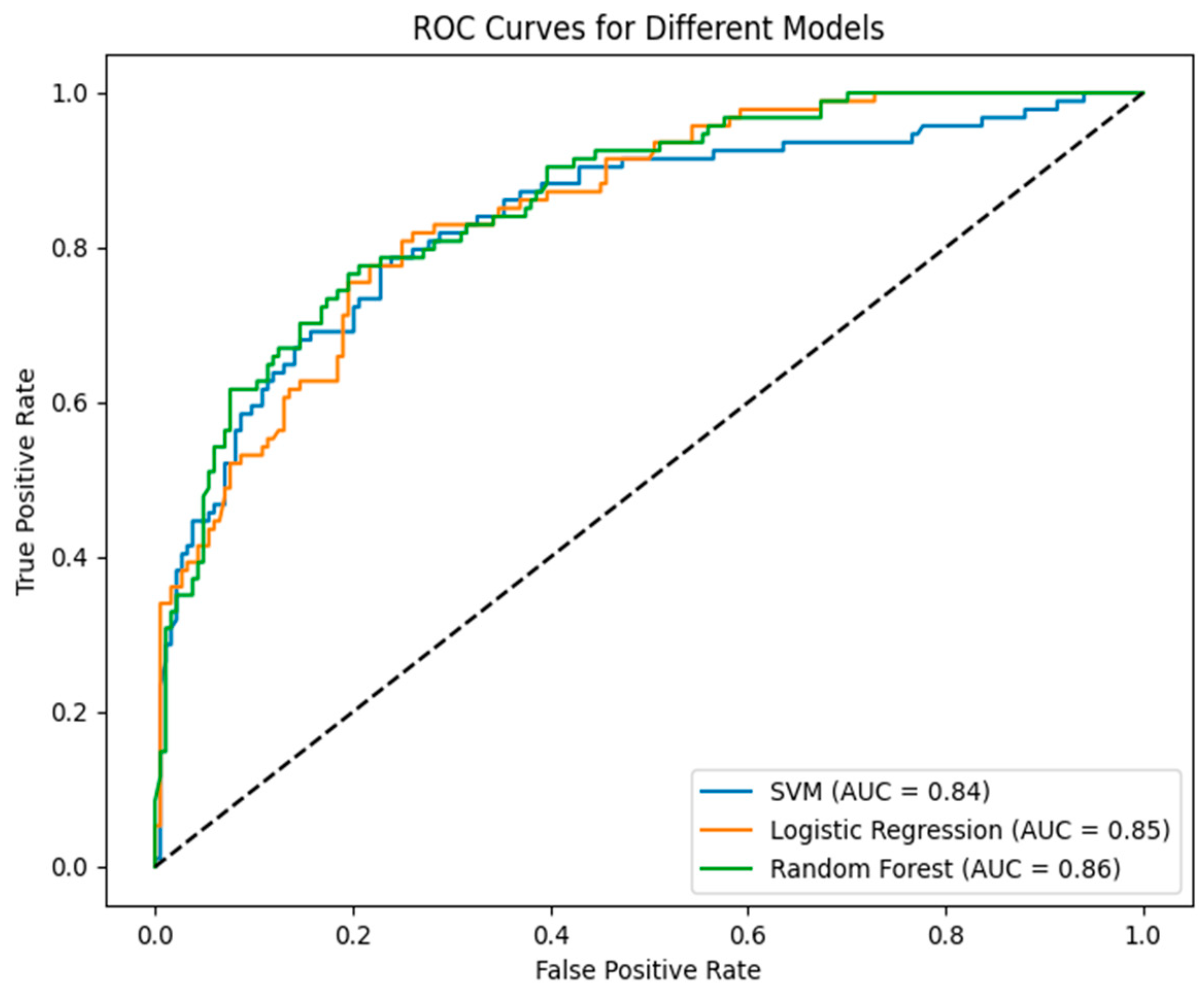
To evaluate the models’ performance and select the best-performing model, several evaluation methods were considered. In addition to the accuracy metric (
Table 5), the Performance Metrics (
Table 6,
Table 7 and
Table 8) and AUC-ROC curve (
Figure 2) were analyzed for each model.
The comparative analysis of evaluation metric results for the three models reveals a close performance proximity in terms of essential metrics, including AUC, precision, recall, and F1-score. This observation suggests that all three models demonstrate proficient predictive capabilities for the binary classification task of discerning whether a child will walk home from school or not. Notably, SVM and RF exhibit marginally higher accuracy than the LR model. Hence, it can be inferred that these two models, SVM and RF, outperform the LR model in this context.
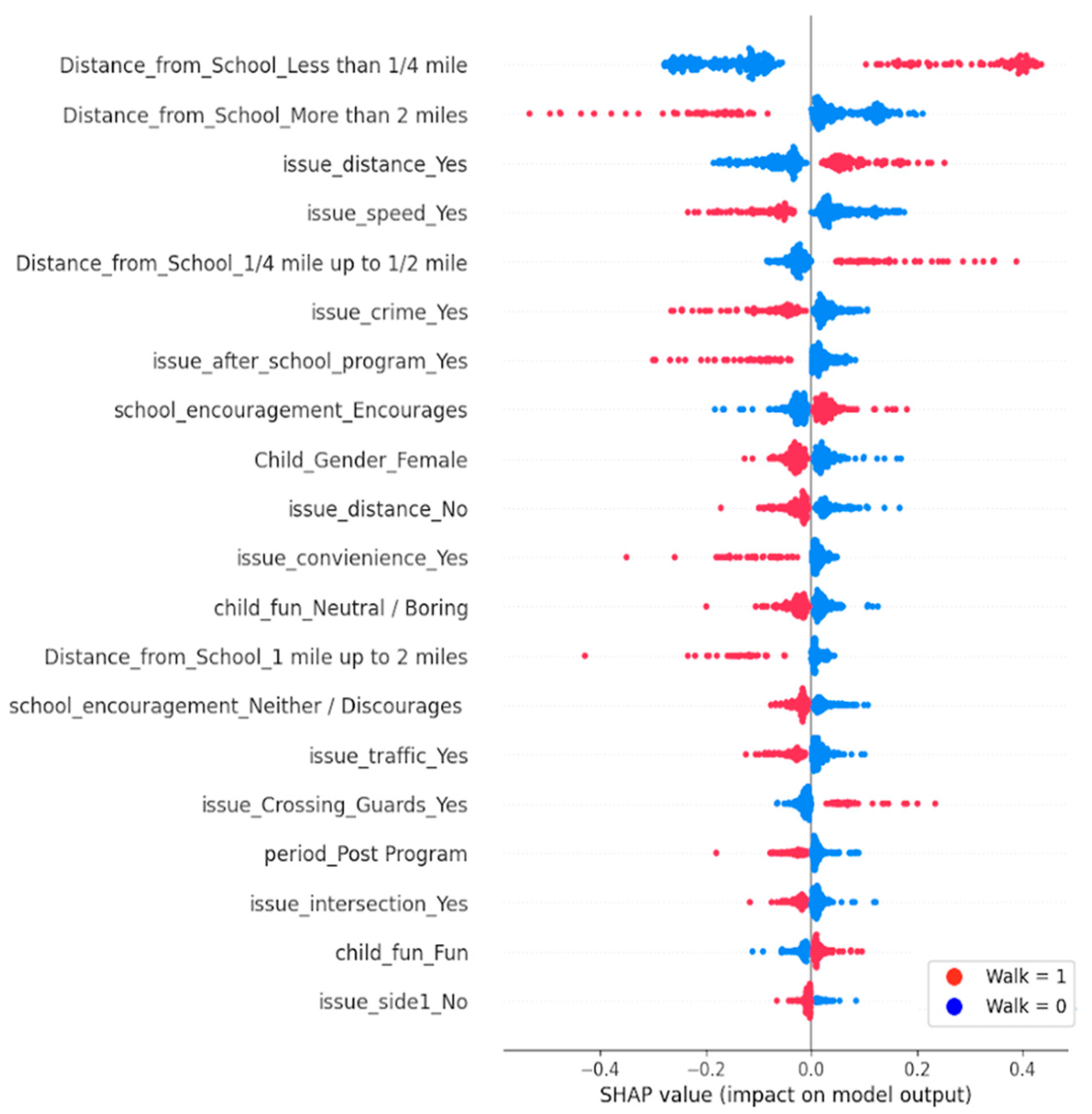
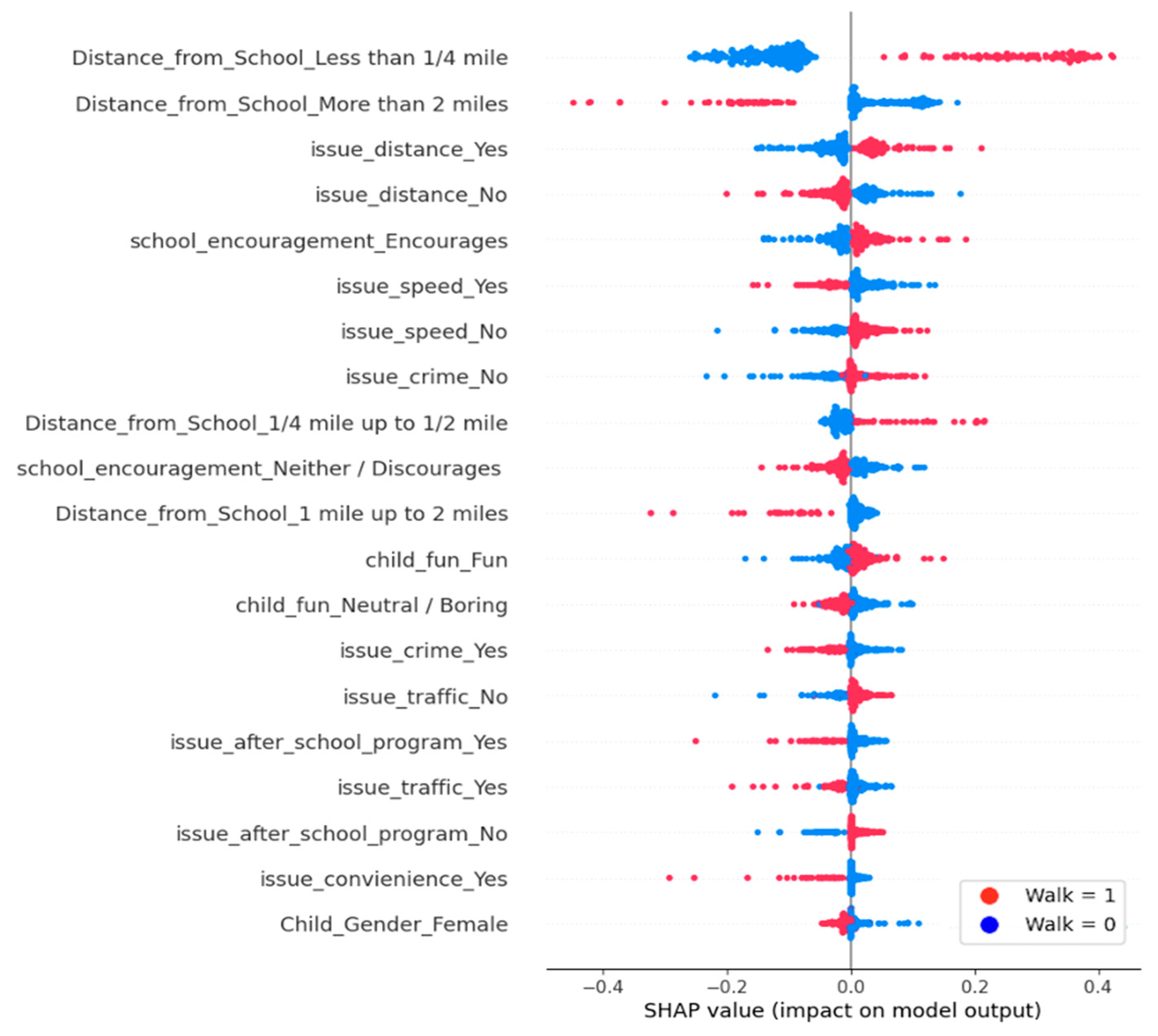
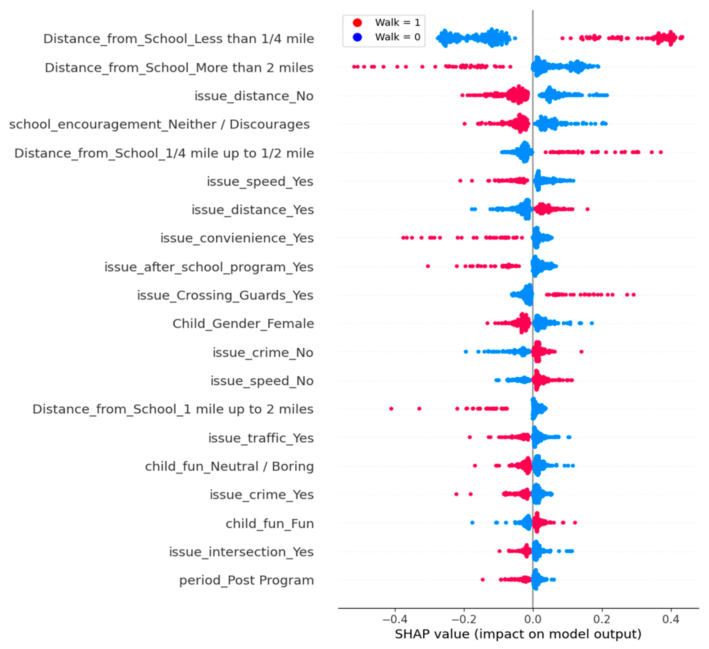
To gain deeper insights into each models’ performance and understand the impact of individual features on ATS, permutation importance (SHAP values) was employed (
Figure 3,
Figure 4 and
Figure 5). By measuring the decrease in model performance when randomly shuffling the values of a particular feature while keeping others unchanged, permutation importance allowed us to identify the features that significantly influenced the model’s predictions [
96].
5. Discussion
Utilizing data from the Safe Routes to School program, this study aims to uncover barriers to active transportation among students in the Chula Vista Elementary School District. The comprehensive analysis of SHAP values for the support vector machines (SVM), random forest (RF), and linear regression (LR) models has provided valuable insights into the factors influencing transportation choices to school. Our study findings align with previous research that has primarily focused on changes in travel behavior associated with SRTS program interventions. The analysis through SHAP values consistently demonstrated similar performances and feature ranking across the three machine learning models.
Aligning with previous studies, our study highlights the crucial role of home-to-school distance in shaping students’ transportation choices. Children and adolescents are more likely to engage in active transportation when the distance between their residential area and school is less than 1/4 of a mile or ranges from 1/4 to ½ of a mile. However, distances exceeding 1/2 a mile, especially those greater than 2 miles, exhibit the highest negative impact on the rate of active transportation to school. However, only around 50% of CVESD students who lived within less than half a mile from the school chose to walk as their primary mode of transportation. Therefore, targeted strategies are required to encourage the remaining 50% to walk to school.
Mediating factors exert a significant influence on students’ decisions regarding active transportation to and from school, with parental perceptions playing a crucial role. Our dataset indicates that 60% of students expressed a willingness to walk or cycle to school, seeking permission from their parents to do so. However, it is notable that only half of this group was observed to actively walk to school, suggesting that parents may have various underlying reasons for their decisions. Results from this study show that parental perceptions of the environment have a strong impact on transportation patterns to school, with concerns about crime rate and speed of traffic along the route as the most significant barriers to active transportation to school. Although factors such as the convenience of driving, after-school programs, safety of intersections and crossings, and traffic along the route display relatively minor influences, they contribute slightly to the negative impact on the ATS rate. The presence of a crossing guard was also found to be a modest positive factor, often convincing more parents to allow their children to opt for active transportation. However, factors that one might anticipate influencing the decision, like concerns over time, the need for adult supervision during the walk, concerns regarding sidewalks and pathways, and weather conditions, surprisingly did not have even a minor impact on parents’ choices.
Moreover, our study underscores the importance of schools’ encouragement in promoting active transportation. Although the SRTS program period was not found to be a significant factor in increasing students’ willingness to walk to school, low levels of ATS encouragement were found to adversely influence walking trends among students. School-based interventions and educational programs that foster positive attitudes towards active transportation can be instrumental in promoting sustainable and health-conscious travel choices among students. Additionally, student perceptions of ATS as uninteresting or boring are associated with reduced likelihoods of walking to school. This highlights the importance of creating engaging and enjoyable mechanisms to encourage students.
Furthermore, our study indicates that the possibility of opting for active transportation appears to be higher among male students compared to their female counterparts. Understanding the underlying reasons for this gender disparity can help inform gender-specific interventions to promote active transportation among female students.
Lastly, a few study limitations should be acknowledged. First, the low number of students riding a bike in our sample led us to exclude bicycle transportation from our analyses, potentially overlooking important factors influencing active transportation trends. Future studies with larger and more diverse datasets, including a sufficient representation of bicycling students, could provide a more comprehensive understanding of the determinants of transportation choices to school. Furthermore, our study focused on individual-level factors, and we did not analyze the influence of the Chula Vista Elementary School District’s built environment on walking trends. Exploring the impact of the built environment, including infrastructure, sidewalk availability, and traffic safety measures, could provide valuable insights into how the surroundings affect active transportation behaviors. Addressing these limitations in future research will further enhance our understanding and inform targeted interventions aimed at fostering sustainable and health-conscious travel choices among students.
6. Conclusions
Leveraging the capabilities of various machine learning models, namely support vector machines (SVM), logistic regression (LR), and random forest (RF), this research utilizes SHAP (SHapley Additive exPlanations) values with the primary objective of understanding the determinants influencing transportation choices among students in the CVESD. SHAP offers a consistent and unified measure to interpret machine learning model outputs, aiding an in-depth, intuitive understanding of model decisions. Using SHAP in this study ensured an unbiased, accurate ranking of factors. The integration of advanced machine learning techniques in conjunction with SHAP contributed to a better understanding of the dynamics of student transportation. By identifying and highlighting barriers to ATS, this study provides policymakers with critical insights essential for crafting comprehensive, sustainable, and inclusive transport strategies. As cities and educational institutions globally strive for sustainable and inclusive transportation policies, understanding these nuanced factors becomes paramount.
A significant observation from the SHAP value rankings is its consistency with prior studies which emphasize the significant role of home-to-school distance in shaping students’ transportation decisions. The data revealed that distances greater than 1/2 a mile, and especially those beyond 2 miles, had a profound negative influence on the likelihood of students choosing active transportation. Proximity to school continues to stand out as a primary determinant in students’ transportation choices. Additionally, mediating factors, particularly parental concerns regarding crime rates and speed of traffic along the route, emerged as critical influencers affecting parents’ willingness to allow their children to engage in active transportation modes.
This study also underscores the importance of schools’ encouragement and interventions in promoting active transportation among students. Evidently, the proactive involvement and policies of a school can significantly influence students’ propensity to adopt active commuting methods. Interestingly, while the specific period of the Safe Routes to School (SRTS) program did not have a marked impact on students’ choices, the overall encouragement from the schools had a pronounced effect. The study also found that even though around 60% of the students showed a willingness to walk, only half of them were actively doing so, revealing a potential gap between student intent and actual behavior. Gender disparities were also noted, with males more inclined to choose active transportation than females. Such gender-based differences prompt a need to further investigate the barriers faced specifically by female students and to tailor strategies accordingly. Furthermore, the performance metrics of our machine learning models showed promising results; both SVM and RF models demonstrated a prediction accuracy of 80%, outperforming the LR model. Such levels of accuracy suggest that the models can reliably predict transportation choices based on the given features.
We recommend that future research endeavors to incorporate larger and more diverse datasets and explore the influence of the built environment on walking behaviors. Such efforts hold the potential to yield valuable insights for targeted interventions aimed at promoting sustainable and health-conscious travel choices among students in the CVESD and similar settings.


 ,
, 


