
Analysis and Modeling of Residential Energy Consumption Profiles Using Device-Level Data: A Case Study of Homes Located in Santiago de Chile
 ,
,
Abstract
:1. Introduction
2. Literature Review
2.1. Empirical Literature on Load Profiles or Consumption Patterns
2.2. Fixed Effects Methodology and Consumption within the Household
2.3. Empirical Literature on Daylight Saving Time
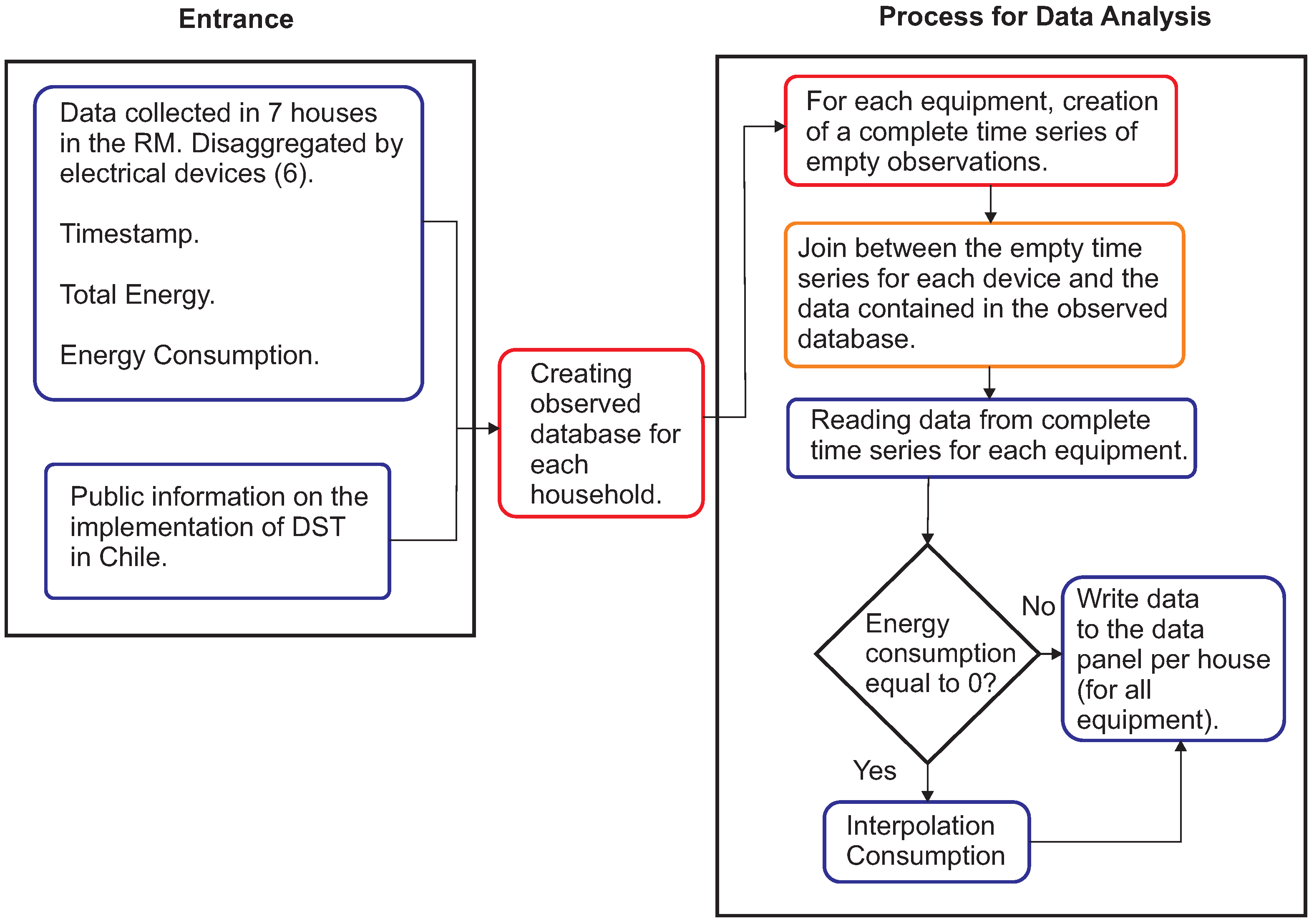
3. Materials and Methods
3.1. Data Manipulation and Cleaning
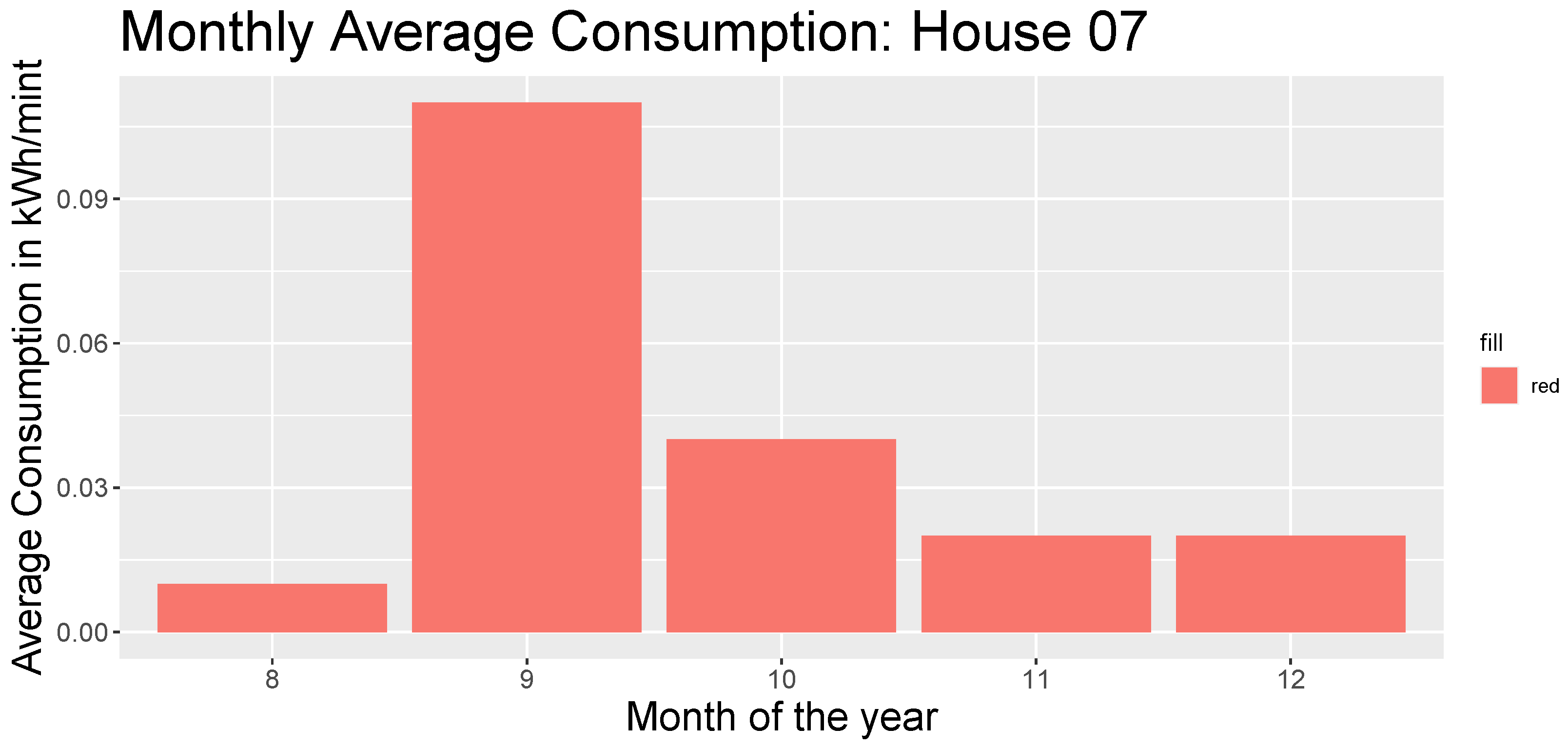
3.2. Descriptive Statistics Analysis
3.3. Empirical Methodology
4. Results and Discussion of the Estimation
4.1. Results of the Explanatory Variables Considered
4.2. Quarterly Model vs. Semi-Annual Model
5. Discussion
6. Conclusions
Author Contributions
Funding
Informed Consent Statement
Data Availability Statement
Conflicts of Interest
Abbreviations
| DiD | Differences in differences |
| DST | Daylight saving time |
| OLS | Ordinary least squares |
| PRF | Population regression function |
Appendix A. Complete Regression Results

| House 1 | House 2 | House 3 | House 4 | House 5 | House 6 | House 7 | |
|---|---|---|---|---|---|---|---|
| h1 | −0.0003 | −0.0001 *** | 0.001 *** | 0.023 | 1.356 *** | −0.073 | −0.002 *** |
| (0.0005) | (0.00003) | (0.0004) | (0.423) | (0.492) | (0.074) | (0.001) | |
| h2 | −0.0001 | −0.0003 *** | −0.00004 | 0.011 | 0.521 | 0.410 *** | −0.003 *** |
| (0.0005) | (0.00002) | (0.0003) | (0.426) | (0.510) | (0.080) | (0.001) | |
| h3 | −0.002 *** | −0.0003 *** | −0.001 *** | −0.378 | −9.289 *** | −0.084 | −0.002 *** |
| (0.0004) | (0.00002) | (0.0003) | (0.414) | (0.542) | (0.075) | (0.001) | |
| h4 | 0.004 *** | −0.0004 *** | −0.001 *** | −0.182 | 1.172 ** | −0.084 | −0.0005 |
| (0.001) | (0.00002) | (0.0002) | (0.424) | (0.495) | (0.075) | (0.001) | |
| h5 | −0.001 ** | −0.0004 *** | −0.002 *** | 0.314 | −1.436 *** | 0.187 *** | −0.003 *** |
| (0.0003) | (0.00002) | (0.0003) | (0.412) | (0.496) | (0.065) | (0.001) | |
| h6 | −0.002 *** | −0.0004 *** | −0.001 *** | 0.016 | −3.054 *** | −0.089 | −0.003 *** |
| (0.0003) | (0.00002) | (0.0002) | (0.428) | (0.542) | (0.074) | (0.001) | |
| h7 | −0.001 *** | −0.0004 *** | −0.001 *** | 0.006 | −0.093 | −0.108 | 0.002 ** |
| (0.0004) | (0.00002) | (0.0002) | (0.428) | (0.527) | (0.075) | (0.001) | |
| h8 | −0.001 *** | −0.0003 *** | −0.001 *** | −0.025 | 0.082 | −0.068 | −0.005 *** |
| (0.0004) | (0.00002) | (0.0002) | (0.428) | (0.524) | (0.074) | (0.001) | |
| h9 | −0.001 *** | −0.0003 *** | −0.0003 | 73.911 *** | 53.812 *** | 0.511 *** | −0.002 ** |
| (0.0003) | (0.00002) | (0.001) | (1.188) | (0.855) | (0.062) | (0.001) | |
| h10 | −0.001 ** | −0.0002 *** | −0.001 * | −2.603 *** | −11.990 *** | −1.194 *** | −0.002 * |
| (0.0003) | (0.00002) | (0.0003) | (0.487) | (0.517) | (0.066) | (0.001) | |
| h11 | −0.001 *** | 0.0001 *** | 0.0003 | −2.076 *** | −1.364 *** | 0.422 *** | −0.0001 |
| (0.0004) | (0.00003) | (0.0003) | (0.498) | (0.453) | (0.063) | (0.001) | |
| h12 | −0.001 *** | 0.0002 *** | −0.001 *** | −2.079 *** | −1.297 ** | 6.305 *** | −0.0003 |
| (0.0004) | (0.00003) | (0.0003) | (0.497) | (0.541) | (0.120) | (0.001) | |
| h13 | −0.00003 | 0.0001 *** | −0.0002 | −1.503 *** | −2.107 *** | −0.288 *** | 0.001 |
| (0.0004) | (0.00003) | (0.001) | (0.410) | (0.502) | (0.063) | (0.001) | |
| h14 | −0.001 ** | 0.0002 *** | −0.001 *** | −4.271 *** | −18.526 *** | 0.574 *** | 0.0002 |
| (0.0004) | (0.00003) | (0.0003) | (0.458) | (0.596) | (0.070) | (0.001) | |
| h15 | −0.001 *** | 0.0003 *** | −0.0004 | −2.123 *** | 5.601 *** | −0.060 | 0.0003 |
| (0.0004) | (0.00003) | (0.0004) | (0.492) | (0.517) | (0.074) | (0.001) | |
| h16 | −0.001 * | 0.0001 *** | −0.001 *** | −1.947 *** | −0.897 * | 0.085 | −0.001 |
| (0.0003) | (0.00003) | (0.0003) | (0.494) | (0.527) | (0.070) | (0.001) | |
| h17 | −0.001 ** | 0.00002 | 0.001 | −2.211 *** | −4.003 *** | −0.110 | 0.001 |
| (0.0003) | (0.00003) | (0.001) | (0.492) | (0.551) | (0.074) | (0.001) | |
| h18 | −0.0004 | −0.00003 | −0.0003 | −1.907 *** | −2.064 *** | −0.110 | 0.0002 |
| (0.0004) | (0.00003) | (0.0003) | (0.497) | (0.472) | (0.074) | (0.001) | |
| h19 | −0.001 | 0.0001 *** | −0.001 ** | −1.644 *** | 0.206 | −0.108 | 0.002 *** |
| (0.0005) | (0.00003) | (0.0003) | (0.448) | (0.504) | (0.073) | (0.001) | |
| h20 | 0.0004 | 0.0004 *** | 0.0003 | −1.889 *** | −0.078 | −0.133 * | 0.005 *** |
| (0.001) | (0.0001) | (0.0004) | (0.502) | (0.521) | (0.074) | (0.001) | |
| h21 | −0.002 *** | 0.001 *** | −0.001 ** | −1.882 *** | −0.961 * | 0.142 ** | 0.011 *** |
| (0.0004) | (0.00003) | (0.0003) | (0.501) | (0.521) | (0.069) | (0.002) | |
| h22 | −0.0004 | 0.001 *** | −0.001 *** | −3.256 *** | −3.918 *** | −1.439 *** | 0.001 ** |
| (0.0004) | (0.00003) | (0.0003) | (0.449) | (0.527) | (0.077) | (0.001) | |
| h23 | −0.003 *** | 0.0002 *** | −0.0004 | −0.053 | −0.413 | 0.390 *** | 0.018 *** |
| (0.0004) | (0.00003) | (0.0003) | (0.535) | (0.510) | (0.066) | (0.002) | |
| Constant | 0.002 *** | 0.001 *** | 0.001 *** | 21.487 *** | 48.485 *** | −0.880 *** | 0.043 *** |
| (0.0003) | (0.00005) | (0.0004) | (0.731) | (1.048) | (0.092) | (0.005) | |
| Observations | 746,259 | 603,075 | 728,203 | 718,326 | 679,465 | 538,216 | 735,553 |
| 0.033 | 0.032 | 0.002 | 0.797 | 0.510 | 0.826 | 0.016 | |
| Adjusted | 0.033 | 0.032 | 0.002 | 0.797 | 0.510 | 0.826 | 0.016 |
| Residual Std. Error | 0.017 (df = 746,191) | 0.002 (df = 603,008) | 0.034 (df = 728,135) | 31.749 (df = 718,258) | 34.593 (df = 679,397) | 2.764 (df = 538,149) | 0.081 (df = 735,485) |
| F Statistic | 378.505 *** (df = 67; 746,191) | 299.483 *** (df = 66; 603,008) | 20.106 *** (df = 67; 728,135) | 42,075.420 *** (df = 67; 718,258) | 10,554.980 *** (df = 67; 679,397) | 38,638.270 *** (df = 66; 538,149) | 182.887 *** (df = 67; 735,485) |
| House 1 | House 2 | House 3 | House 4 | House 5 | House 6 | House 7 | |
|---|---|---|---|---|---|---|---|
| D2 | −0.003 *** | −0.0002 *** | 0.0002 | 6.259 *** | 14.388 *** | −2.960 *** | −0.029 *** |
| (0.0002) | (0.00004) | (0.0002) | (0.581) | (0.614) | (0.095) | (0.004) | |
| D3 | −0.001 *** | −0.0001 ** | 0.001 *** | 5.791 *** | −1.271 * | −1.364 *** | −0.027 *** |
| (0.0001) | (0.00004) | (0.0002) | (0.540) | (0.719) | (0.099) | (0.004) | |
| D4 | −0.002 *** | −0.0001 * | −0.0001 | 1.831 *** | −2.536 *** | −1.708 *** | −0.030 *** |
| (0.0001) | (0.00004) | (0.0002) | (0.559) | (0.722) | (0.094) | (0.004) | |
| D5 | −0.003 *** | −0.0002 *** | 0.001 *** | 10.011 *** | 4.514 *** | −1.853 *** | −0.030 *** |
| (0.0003) | (0.00003) | (0.0002) | (0.507) | (0.669) | (0.088) | (0.004) | |
| D6 | −0.003 *** | −0.0002 *** | −0.0002 | −0.176 | −1.426 | −0.076 | −0.027 *** |
| (0.0002) | (0.00004) | (0.0002) | (0.722) | (0.922) | (0.085) | (0.004) | |
| D7 | −0.001 *** | −0.0002 *** | −0.0003 ** | 3.015 *** | −1.635 * | 0.264 *** | −0.030 *** |
| (0.0002) | (0.00004) | (0.0001) | (0.649) | (0.864) | (0.099) | (0.004) | |
| D8 | −0.0002 | −0.0002 *** | −0.0004 ** | −0.309 | −1.561 *** | 0.086 | −0.026 *** |
| (0.0001) | (0.00004) | (0.0002) | (0.456) | (0.605) | (0.083) | (0.004) | |
| D9 | −0.003 *** | −0.0004 *** | −0.0001 | 6.827 *** | −1.248 ** | −0.302 *** | −0.032 *** |
| (0.0002) | (0.00004) | (0.0002) | (0.494) | (0.628) | (0.081) | (0.004) | |
| D10 | −0.003 *** | −0.0003 *** | 0.003 *** | 1.207 * | −0.747 | 0.251 *** | −0.028 *** |
| (0.0002) | (0.00004) | (0.0005) | (0.654) | (0.857) | (0.086) | (0.004) | |
| D11 | 0.008 *** | −0.0002 *** | −0.00002 | 2.032 *** | −0.498 | 2.158 *** | −0.026 *** |
| (0.001) | (0.00003) | (0.0001) | (0.687) | (0.948) | (0.119) | (0.004) | |
| D12 | −0.002 *** | −0.0003 *** | 0.003 *** | 106.498 *** | 41.317 *** | −0.712 *** | −0.029 *** |
| (0.0002) | (0.00004) | (0.001) | (1.324) | (0.885) | (0.083) | (0.004) | |
| D13 | −0.003 *** | −0.0004 *** | −0.0005 *** | −5.662 *** | −3.748 *** | 0.0005 | −0.026 *** |
| (0.0002) | (0.00004) | (0.0001) | (0.589) | (0.756) | (0.087) | (0.005) | |
| D14 | −0.002 *** | −0.0002 *** | 0.0002 | −2.701 *** | −2.567 *** | 0.929 *** | −0.030 *** |
| (0.0002) | (0.00004) | (0.0002) | (0.685) | (0.791) | (0.087) | (0.004) | |
| D15 | −0.002 *** | −0.0005 *** | −0.0003 ** | 0.0004 | 2.174 *** | −0.235 *** | −0.024 *** |
| (0.0001) | (0.00003) | (0.0002) | (0.549) | (0.743) | (0.078) | (0.004) | |
| D16 | −0.003 *** | −0.0005 *** | 0.001 *** | −1.582 ** | −0.988 | −0.823 *** | −0.024 *** |
| (0.0002) | (0.00004) | (0.0003) | (0.655) | (0.765) | (0.089) | (0.004) | |
| D17 | −0.002 *** | −0.0004 *** | 0.002 *** | −6.040 *** | −5.323 *** | 0.313 *** | −0.026 *** |
| (0.0001) | (0.00004) | (0.0004) | (0.609) | (0.813) | (0.085) | (0.004) | |
| D18 | −0.003 *** | −0.0001 *** | 0.003 *** | −4.878 *** | −2.077 *** | 0.341 *** | −0.028 *** |
| (0.0002) | (0.00004) | (0.0004) | (0.554) | (0.710) | (0.087) | (0.004) | |
| D19 | 0.001 *** | −0.0002 *** | 0.001 *** | 4.212 *** | 2.730 *** | −0.658 *** | −0.028 *** |
| (0.0001) | (0.00004) | (0.0003) | (0.613) | (0.742) | (0.084) | (0.004) | |
| D20 | −0.003 *** | −0.0003 *** | 0.00003 | −5.824 *** | −19.028 *** | 0.098 | −0.025 *** |
| (0.0002) | (0.00004) | (0.0001) | (0.596) | (0.715) | (0.088) | (0.004) | |
| D21 | 0.004 *** | −0.00000 | 0.002 | −7.136 *** | 8.911 *** | 15.557 *** | −0.030 *** |
| (0.001) | (0.00003) | (0.002) | (0.593) | (0.865) | (0.184) | (0.004) | |
| D22 | 0.002 *** | −0.0004 *** | −0.0001 | −0.246 | 5.374 *** | −0.218 *** | −0.028 *** |
| (0.001) | (0.00003) | (0.0001) | (0.546) | (0.698) | (0.078) | (0.004) | |
| D23 | −0.003 *** | −0.0002 *** | −0.0002 | −2.400 *** | 3.319 *** | −0.405 *** | −0.029 *** |
| (0.0002) | (0.00004) | (0.0003) | (0.648) | (0.783) | (0.084) | (0.004) | |
| D24 | −0.002 *** | −0.0003 *** | 0.001 * | −4.987 *** | −7.983 *** | 0.590 *** | −0.027 *** |
| (0.0002) | (0.00004) | (0.001) | (0.603) | (0.734) | (0.078) | (0.004) | |
| D25 | −0.0004 *** | −0.00005 | −0.001 *** | −4.884 *** | 8.857 *** | −0.555 *** | −0.029 *** |
| (0.0001) | (0.00004) | (0.0002) | (0.556) | (0.603) | (0.092) | (0.004) | |
| D26 | −0.003 *** | −0.0004 *** | 0.001 *** | 2.025 *** | 11.593 *** | −0.285 *** | −0.030 *** |
| (0.0002) | (0.00004) | (0.0002) | (0.577) | (0.688) | (0.081) | (0.004) | |
| D27 | −0.002 *** | −0.0005 *** | 0.004 ** | −5.125 *** | 5.197 *** | −0.004 | 0.001 |
| (0.0002) | (0.00004) | (0.002) | (0.609) | (0.683) | (0.088) | (0.004) | |
| D28 | −0.001 *** | −0.0002 *** | −0.0001 | −4.520 *** | 1.212 | 1.111 *** | −0.028 *** |
| (0.0002) | (0.00004) | (0.0001) | (0.586) | (0.772) | (0.089) | (0.004) | |
| D29 | −0.001 *** | −0.0003 *** | −0.0003 * | 0.769 | 4.941 *** | −0.719 *** | −0.026 *** |
| (0.0002) | (0.00003) | (0.0002) | (0.625) | (0.732) | (0.083) | (0.004) | |
| D30 | −0.003 *** | −0.0004 *** | −0.0001 | 9.435 *** | 1.931 ** | −0.349 *** | −0.029 *** |
| (0.0002) | (0.00004) | (0.0002) | (0.719) | (0.799) | (0.083) | (0.004) | |
| D31 | 0.004 *** | −0.0001 *** | 0.001 *** | −16.381 *** | −3.371 *** | 6.453 *** | −0.029 *** |
| (0.0003) | (0.00004) | (0.0002) | (0.789) | (1.004) | (0.133) | (0.004) | |
| Constant | 0.002 *** | 0.001 *** | 0.001 *** | 21.487 *** | 48.485 *** | −0.880 *** | 0.043 *** |
| (0.0003) | (0.00005) | (0.0004) | (0.731) | (1.048) | (0.092) | (0.005) | |
| Observations | 746,259 | 603,075 | 728,203 | 718,326 | 679,465 | 538,216 | 735,553 |
| 0.033 | 0.032 | 0.002 | 0.797 | 0.510 | 0.826 | 0.016 | |
| Adjusted | 0.033 | 0.032 | 0.002 | 0.797 | 0.510 | 0.826 | 0.016 |
| Residual Std. Error | 0.017 (df = 746,191) | 0.002 (df = 603,008) | 0.034 (df = 728,135) | 31.749 (df = 718,258) | 34.593 (df = 679,397) | 2.764 (df = 538,149) | 0.081 (df = 735,485) |
| F Statistic | 378.505 *** (df = 67; 746,191) | 299.483 *** (df = 66; 603,008) | 20.106 *** (df = 67; 728,135) | 42,075.420 *** (df = 67; 718,258) | 10,554.980 *** (df = 67; 679,397) | 38,638.270 *** (df = 66; 538,149) | 182.887 *** (df = 67; 735,485) |
| House 1 | House 2 | House 3 | House 4 | House 5 | House 6 | House 7 | |
|---|---|---|---|---|---|---|---|
| h1 | −0.00000 | −0.0001 | 0.0004 ** | 0.035 *** | −0.002 | −0.019 | −0.002 *** |
| (0.0004) | (0.0001) | (0.0002) | (0.005) | (0.001) | (0.038) | (0.001) | |
| h2 | 0.0001 | −0.0004 *** | −0.0001 | −0.040 *** | −0.002 | −1.608 *** | −0.003 *** |
| (0.0004) | (0.0001) | (0.0001) | (0.005) | (0.002) | (0.045) | (0.001) | |
| h3 | −0.001 *** | −0.0004 *** | −0.001 *** | −0.050 *** | 0.006 ** | 0.520 *** | 0.0005 |
| (0.0003) | (0.0001) | (0.0001) | (0.006) | (0.003) | (0.049) | (0.001) | |
| h4 | 0.004 *** | −0.0004 *** | −0.001 *** | −0.049 *** | 0.014 *** | −0.002 | −0.001 * |
| (0.0005) | (0.0001) | (0.0001) | (0.006) | (0.003) | (0.039) | (0.001) | |
| h5 | −0.0004 | −0.0004 *** | −0.001 *** | 0.007 | −0.005 *** | 0.078 ** | 0.002 * |
| (0.0003) | (0.0001) | (0.0001) | (0.007) | (0.001) | (0.034) | (0.001) | |
| h6 | −0.001 *** | −0.0004 *** | −0.001 *** | −0.038 *** | −0.003 * | −0.011 | −0.003 *** |
| (0.0003) | (0.0001) | (0.0001) | (0.005) | (0.002) | (0.039) | (0.001) | |
| h7 | −0.001 *** | −0.0004 *** | −0.001 *** | −0.033 *** | −0.004 *** | 0.035 | −0.003 *** |
| (0.0003) | (0.0001) | (0.0001) | (0.005) | (0.001) | (0.038) | (0.001) | |
| h8 | −0.001 *** | −0.0003 *** | −0.001 *** | −0.017 *** | −0.014 *** | 0.045 | 0.001 |
| (0.0003) | (0.0001) | (0.0001) | (0.006) | (0.002) | (0.035) | (0.002) | |
| h9 | −0.001 *** | −0.0002 *** | 0.001 * | 0.056 *** | 0.008 | 0.350 *** | −0.0002 |
| (0.0003) | (0.0001) | (0.0004) | (0.013) | (0.008) | (0.032) | (0.001) | |
| h10 | −0.001 * | −0.0001 | 0.002 ** | −0.002 | 0.0004 | −1.431 *** | 0.001 |
| (0.0003) | (0.0001) | (0.001) | (0.008) | (0.001) | (0.040) | (0.001) | |
| h11 | −0.001 *** | 0.0005 *** | 0.0005 * | 0.005 | 0.005 | 0.168 *** | 0.002 *** |
| (0.0003) | (0.0001) | (0.0003) | (0.007) | (0.003) | (0.033) | (0.001) | |
| h12 | −0.001 ** | 0.003 *** | 0.0001 | 0.027 *** | 0.003 * | 5.082 *** | 0.002 *** |
| (0.0003) | (0.0003) | (0.0001) | (0.008) | (0.002) | (0.065) | (0.001) | |
| h13 | 0.001 *** | 0.001 *** | 0.001 | 0.004 | −0.002 | 0.166 *** | 0.004 *** |
| (0.0003) | (0.0001) | (0.0004) | (0.005) | (0.002) | (0.031) | (0.001) | |
| h14 | −0.001 *** | 0.001 *** | −0.0004 *** | 0.002 | 0.003 * | 0.406 *** | 0.003 *** |
| (0.0003) | (0.0001) | (0.0001) | (0.007) | (0.002) | (0.036) | (0.001) | |
| h15 | −0.001 ** | 0.001 *** | −0.0004 *** | −0.077 *** | 0.010 *** | −0.005 | 0.003 *** |
| (0.0003) | (0.0001) | (0.0001) | (0.006) | (0.002) | (0.035) | (0.001) | |
| h16 | −0.0004 | 0.001 *** | −0.0001 | 0.021 *** | −0.002 | −0.112 *** | 0.002 *** |
| (0.0003) | (0.0001) | (0.0001) | (0.005) | (0.002) | (0.041) | (0.001) | |
| h17 | −0.001 * | 0.001 *** | 0.001 | −0.014 ** | −0.007 *** | −0.106 ** | 0.003 *** |
| (0.0003) | (0.0001) | (0.0004) | (0.007) | (0.002) | (0.042) | (0.001) | |
| h18 | −0.0003 | −0.001 *** | 0.0003 ** | 0.012 * | −0.004 *** | −0.050 | 0.007 *** |
| (0.0004) | (0.0001) | (0.0002) | (0.006) | (0.002) | (0.039) | (0.001) | |
| h19 | −0.0003 | 0.003 *** | 0.0003 * | −0.078 *** | −0.004 *** | −0.155 *** | 0.003 *** |
| (0.0004) | (0.0002) | (0.0001) | (0.010) | (0.001) | (0.042) | (0.001) | |
| h20 | 0.0004 | 0.004 *** | 0.0004 *** | −0.018 *** | −0.001 | 0.085 ** | 0.007 *** |
| (0.0005) | (0.0002) | (0.0002) | (0.006) | (0.002) | (0.035) | (0.001) | |
| h21 | −0.001 *** | 0.004 *** | 0.001 *** | −0.016 *** | 0.001 | 0.070 * | 0.012 *** |
| (0.0004) | (0.0002) | (0.0002) | (0.006) | (0.006) | (0.037) | (0.002) | |
| h22 | −0.0001 | 0.002 *** | 0.001 *** | −0.017 *** | 0.003 | −0.823 *** | 0.061 *** |
| (0.0004) | (0.0002) | (0.0001) | (0.005) | (0.002) | (0.038) | (0.003) | |
| h23 | −0.003 *** | 0.001 *** | −0.0002 | 1.165 *** | −0.005 *** | 0.046 | 0.014 *** |
| (0.0004) | (0.0001) | (0.0001) | (0.114) | (0.001) | (0.036) | (0.001) | |
| holidays | −0.004 | 0.0003 ** | −0.0003 *** | 0.020 *** | 0.003 * | −3.080 *** | 0.031 *** |
| (0.0003) | (0.0001) | (0.0001) | (0.006) | (0.002) | (0.047) | (0.002) | |
| dst | −0.0002 | −0.001 *** | 0.0001 | 0.054 *** | 0.009 *** | −2.190 *** | 0.019 *** |
| (0.00002) | (0.0001) | (0.0002) | (0.007) | (0.002) | (0.044) | (0.002) | |
| Constant | 0.003 *** | 0.006 *** | 0.002 *** | 0.191 *** | 0.024 *** | −1.481 *** | −0.013 *** |
| (0.0004) | (0.0002) | (0.0002) | (0.010) | (0.002) | (0.064) | (0.003) | |
| Observations | 1,633,802 | 1,783,481 | 1,749,531 | 1,672,655 | 1,648,740 | 1,304,140 | 1,653,857 |
| 0.067 | 0.024 | 0.001 | 0.030 | 0.002 | 0.657 | 0.036 | |
| Adjusted | 0.067 | 0.024 | 0.0005 | 0.030 | 0.002 | 0.656 | 0.036 |
| Residual Std. Error | 0.011 (df = 1,633,732) | 0.014 (df = 1,783,409) | 0.043 (df = 1,749,459) | 1.787 (df = 1,672,583) | 0.330 (df = 1,648,668) | 2.533 (df = 1,304,068) | 0.107 (df = 1,653,786) |
| F Statistic | 1706.848 *** (df = 69; 1,633,732) | 614.282 *** (df = 71; 1,783,409) | 12.813 *** (df = 71; 1,749,459) | 732.879 *** (df = 71; 1,672,583) | 38.180 *** (df = 71; 1,648,668) | 35,103.650 *** (df = 71; 1,304,068) | 875.066 *** (df = 70; 1,653,786) |
| House 1 | House 2 | House 3 | House 4 | House 5 | House 6 | House 7 | |
|---|---|---|---|---|---|---|---|
| D2 | −0.002 *** | 0.00003 | 0.0004 * | 0.017 ** | 0.004 *** | −2.044 *** | −0.004 |
| (0.0002) | (0.0001) | (0.0002) | (0.007) | (0.001) | (0.063) | (0.003) | |
| D3 | −0.001 *** | −0.0002 | 0.0002 ** | −0.035 *** | 0.010 *** | −0.002 | −0.001 |
| (0.0001) | (0.0001) | (0.0001) | (0.011) | (0.003) | (0.060) | (0.003) | |
| D4 | −0.002 *** | 0.00002 | 0.0005 *** | 0.062 *** | 0.030 *** | −0.368 *** | −0.010 *** |
| (0.0001) | (0.0001) | (0.0001) | (0.006) | (0.005) | (0.067) | (0.003) | |
| D5 | −0.002 *** | −0.0004 *** | 0.0003 *** | 0.0001 | 0.004 ** | −0.251 *** | −0.025 *** |
| (0.0002) | (0.0001) | (0.0001) | (0.007) | (0.002) | (0.064) | (0.003) | |
| D6 | −0.002 *** | 0.0001 | −0.0001 | −0.029 | −0.002 * | 0.756 *** | −0.016 *** |
| (0.0001) | (0.0001) | (0.0001) | (0.019) | (0.001) | (0.057) | (0.003) | |
| D7 | −0.002 *** | 0.00000 | 0.001 *** | 0.068 *** | 0.016 *** | 0.869 *** | −0.006 * |
| (0.0002) | (0.0001) | (0.0002) | (0.007) | (0.003) | (0.065) | (0.003) | |
| D8 | −0.001 *** | 0.0004 ** | −0.0004 *** | 0.050 *** | 0.002 | −0.117 * | −0.016 *** |
| (0.0001) | (0.0002) | (0.0001) | (0.005) | (0.002) | (0.064) | (0.003) | |
| D9 | −0.002 *** | 0.001 *** | −0.0001 | −0.005 | 0.002 ** | 1.422 *** | −0.010 *** |
| (0.0002) | (0.0002) | (0.0001) | (0.006) | (0.001) | (0.055) | (0.004) | |
| D10 | −0.003 *** | 0.001 *** | 0.001 *** | 0.025 *** | −0.001 | 1.257 *** | −0.008 ** |
| (0.0002) | (0.0002) | (0.0002) | (0.005) | (0.001) | (0.056) | (0.004) | |
| (0.001) | (0.0002) | (0.0001) | (0.008) | (0.001) | (0.063) | (0.003) | |
| D12 | −0.001 *** | 0.001 *** | 0.001 *** | −0.015 | 0.012 | 1.575 *** | −0.003 |
| (0.0001) | (0.0002) | (0.0005) | (0.018) | (0.008) | (0.055) | (0.003) | |
| D13 | −0.002 *** | 0.001 *** | 0.001 *** | −0.053 *** | −0.005 *** | 0.913 *** | −0.010 *** |
| (0.0002) | (0.0002) | (0.0003) | (0.011) | (0.001) | (0.058) | (0.004) | |
| D14 | −0.002 *** | 0.001 *** | 0.00001 | 1.209 *** | −0.002 | 1.384 *** | −0.008 ** |
| (0.0001) | (0.0002) | (0.0001) | (0.115) | (0.001) | (0.056) | (0.003) | |
| D15 | −0.001 *** | 0.001 *** | 0.0003 *** | −0.051 *** | −0.002 | 2.087 *** | −0.009 ** |
| (0.0001) | (0.0002) | (0.0001) | (0.011) | (0.001) | (0.057) | (0.003) | |
| D16 | −0.002 *** | −0.0002 | 0.001 *** | −0.025 * | −0.003 *** | 1.081 *** | −0.009 *** |
| (0.0001) | (0.0001) | (0.0001) | (0.013) | (0.001) | (0.058) | (0.003) | |
| D17 | −0.002 *** | −0.0004 *** | −0.0001 | −0.049 *** | −0.006 *** | 1.859 *** | −0.007 ** |
| (0.0001) | (0.0001) | (0.0001) | (0.011) | (0.001) | (0.059) | (0.003) | |
| D18 | −0.002 *** | −0.0002 ** | 0.001 *** | 0.033 *** | −0.002 | 1.794 *** | −0.009 ** |
| (0.0001) | (0.0001) | (0.0002) | (0.008) | (0.003) | (0.058) | (0.004) | |
| D19 | 0.00002 | 0.002 *** | 0.0004 *** | −0.054 *** | 0.002 | 1.703 *** | 0.054 *** |
| (0.0001) | (0.0004) | (0.0001) | (0.012) | (0.001) | (0.059) | (0.005) | |
| D20 | −0.002 *** | 0.0003 ** | −0.0003 *** | −0.047 *** | 0.008 *** | 0.844 *** | −0.012 *** |
| (0.0002) | (0.0002) | (0.0001) | (0.012) | (0.001) | (0.058) | (0.003) | |
| D21 | 0.004 *** | 0.001 *** | 0.0002 | 0.024 *** | 0.006 | 11.271 *** | −0.014 *** |
| (0.001) | (0.0002) | (0.0003) | (0.008) | (0.004) | (0.126) | (0.003) | |
| D22 | 0.002 *** | 0.0002 | −0.0003 *** | 0.032 *** | 0.011 ** | 1.332 *** | −0.006 * |
| (0.001) | (0.0001) | (0.0001) | (0.008) | (0.004) | (0.055) | (0.003) | |
| D23 | −0.002 *** | 0.0004 *** | −0.0003 *** | 0.028 ** | −0.002 ** | 1.479 *** | −0.010 *** |
| (0.0001) | (0.0001) | (0.0001) | (0.014) | (0.001) | (0.056) | (0.003) | |
| D24 | −0.002 *** | 0.0002 * | 0.001 ** | 0.041 *** | −0.004 *** | 1.381 *** | 0.0005 |
| (0.0001) | (0.0001) | (0.0002) | (0.010) | (0.001) | (0.055) | (0.003) | |
| D25 | −0.001 *** | 0.0003 * | 0.0005 | 0.013 | −0.004 ** | 1.105 *** | −0.017 *** |
| (0.0001) | (0.0001) | (0.0003) | (0.012) | (0.002) | (0.057) | (0.003) | |
| D26 | −0.001 *** | 0.0004 ** | 0.001 *** | −0.105 *** | 0.007 ** | 1.539 *** | −0.006 * |
| (0.0001) | (0.0002) | (0.0002) | (0.018) | (0.003) | (0.056) | (0.003) | |
| D27 | −0.001 *** | −0.002 *** | 0.001 ** | −0.046 *** | −0.0003 | 1.287 *** | 0.018 *** |
| (0.0001) | (0.0001) | (0.001) | (0.010) | (0.005) | (0.055) | (0.004) | |
| D28 | −0.001 *** | 0.001 *** | 0.001 | −0.091 *** | −0.002 * | 1.388 *** | −0.004 |
| (0.0002) | (0.0002) | (0.001) | (0.013) | (0.001) | (0.057) | (0.003) | |
| D29 | −0.001 *** | 0.0005 *** | 0.00003 | 0.021 *** | 0.002 * | 0.998 *** | 0.0002 |
| (0.0002) | (0.0002) | (0.0001) | (0.005) | (0.001) | (0.056) | (0.004) | |
| D30 | −0.001 *** | 0.0003 ** | 0.0001 | −0.073 *** | −0.003 ** | 1.384 *** | −0.013 *** |
| (0.0001) | (0.0001) | (0.0001) | (0.018) | (0.001) | (0.056) | (0.003) | |
| D31 | 0.003 *** | −0.001 *** | −0.0001 | −0.129 *** | −0.005 *** | 2.143 *** | −0.019 *** |
| (0.0002) | (0.0001) | (0.0001) | (0.016) | (0.002) | (0.060) | (0.003) | |
| Constant | 0.003 *** | 0.006 *** | 0.002 *** | 0.191 *** | 0.024 *** | −1.481 *** | −0.013 *** |
| (0.0004) | (0.0002) | (0.0002) | (0.010) | (0.002) | (0.064) | (0.003) | |
| Observations | 1,633,802 | 1,783,481 | 1,749,531 | 1,672,655 | 1,648,740 | 1,304,140 | 1,653,857 |
| 0.067 | 0.024 | 0.001 | 0.030 | 0.002 | 0.657 | 0.036 | |
| Adjusted | 0.067 | 0.024 | 0.0005 | 0.030 | 0.002 | 0.656 | 0.036 |
| Residual Std. Error | 0.011 (df = 1,633,732) | 0.014 (df = 1,783,409) | 0.043 (df = 1,749,459) | 1.787 (df = 1,672,583) | 0.330 (df = 1,648,668) | 2.533 (df = 1,304,068) | 0.107 (df = 1,653,786) |
| F Statistic | 1706.848 *** (df = 69; 1,633,732) | 614.282 *** (df = 71; 1,783,409) | 12.813 *** (df = 71; 1,749,459) | 732.879 *** (df = 71; 1,672,583) | 38.180 *** (df = 71; 1,648,668) | 35,103.650 *** (df = 71; 1,304,068) | 875.066 *** (df = 70; 1,653,786) |
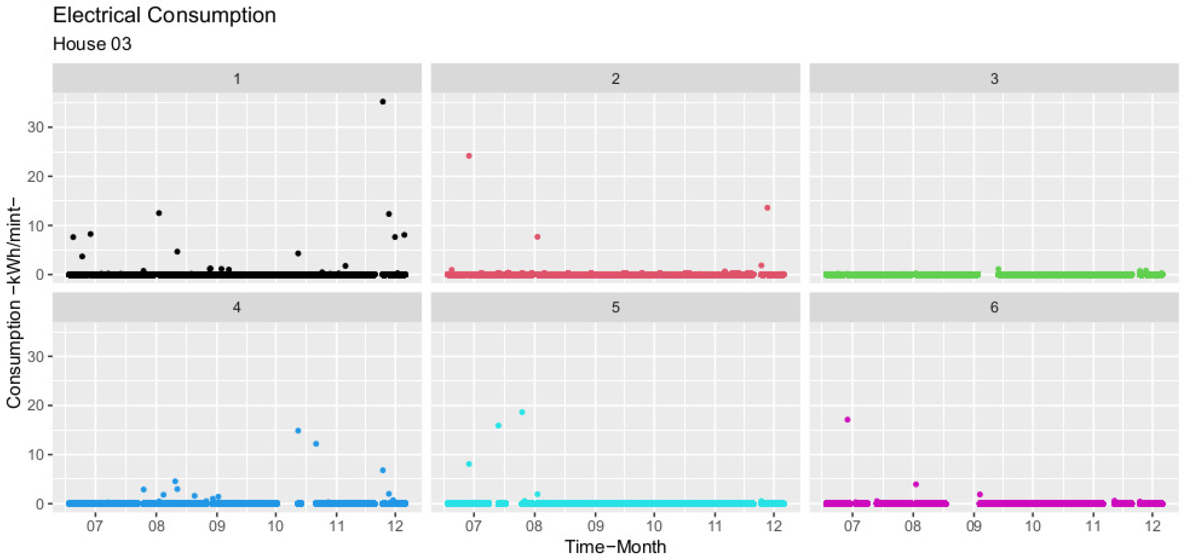
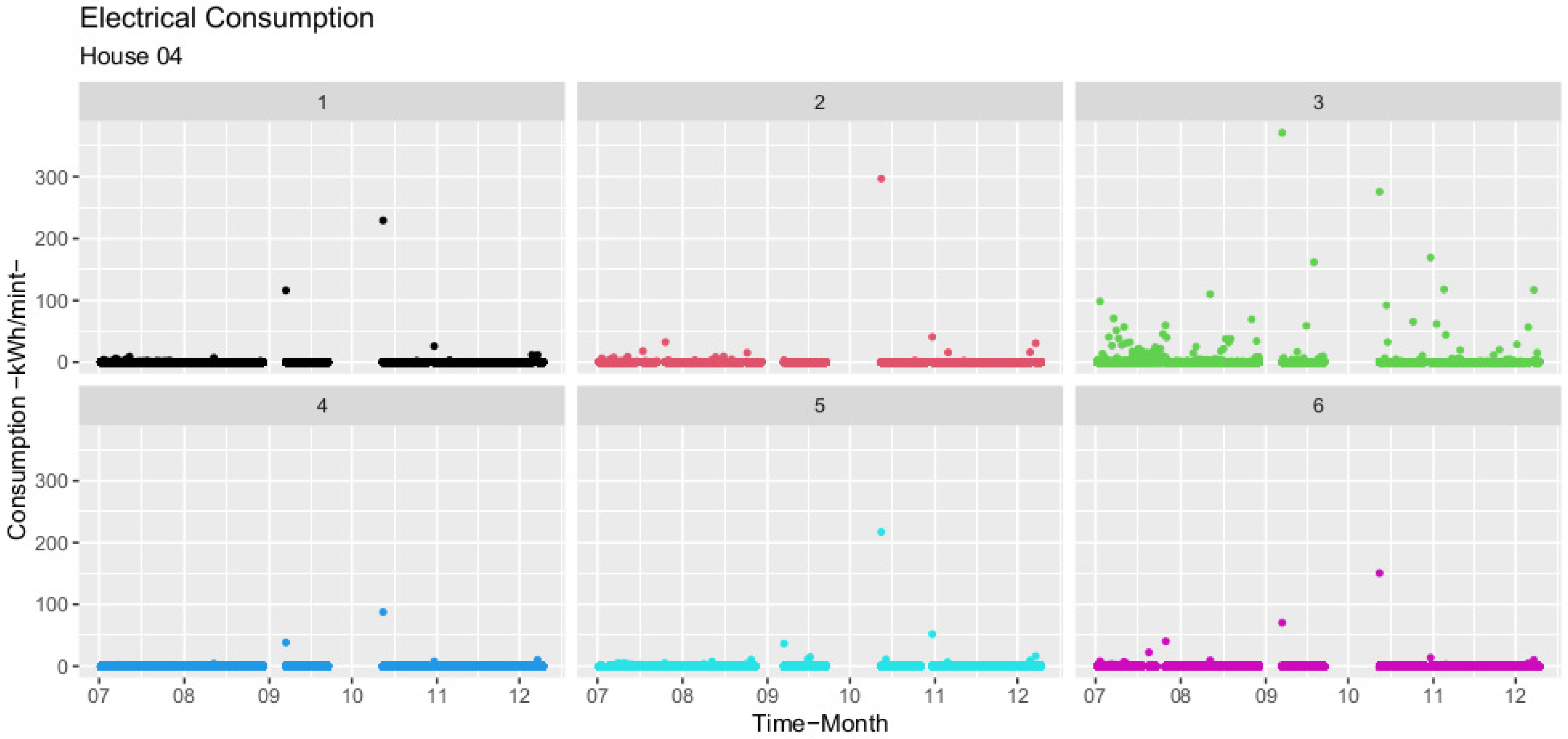
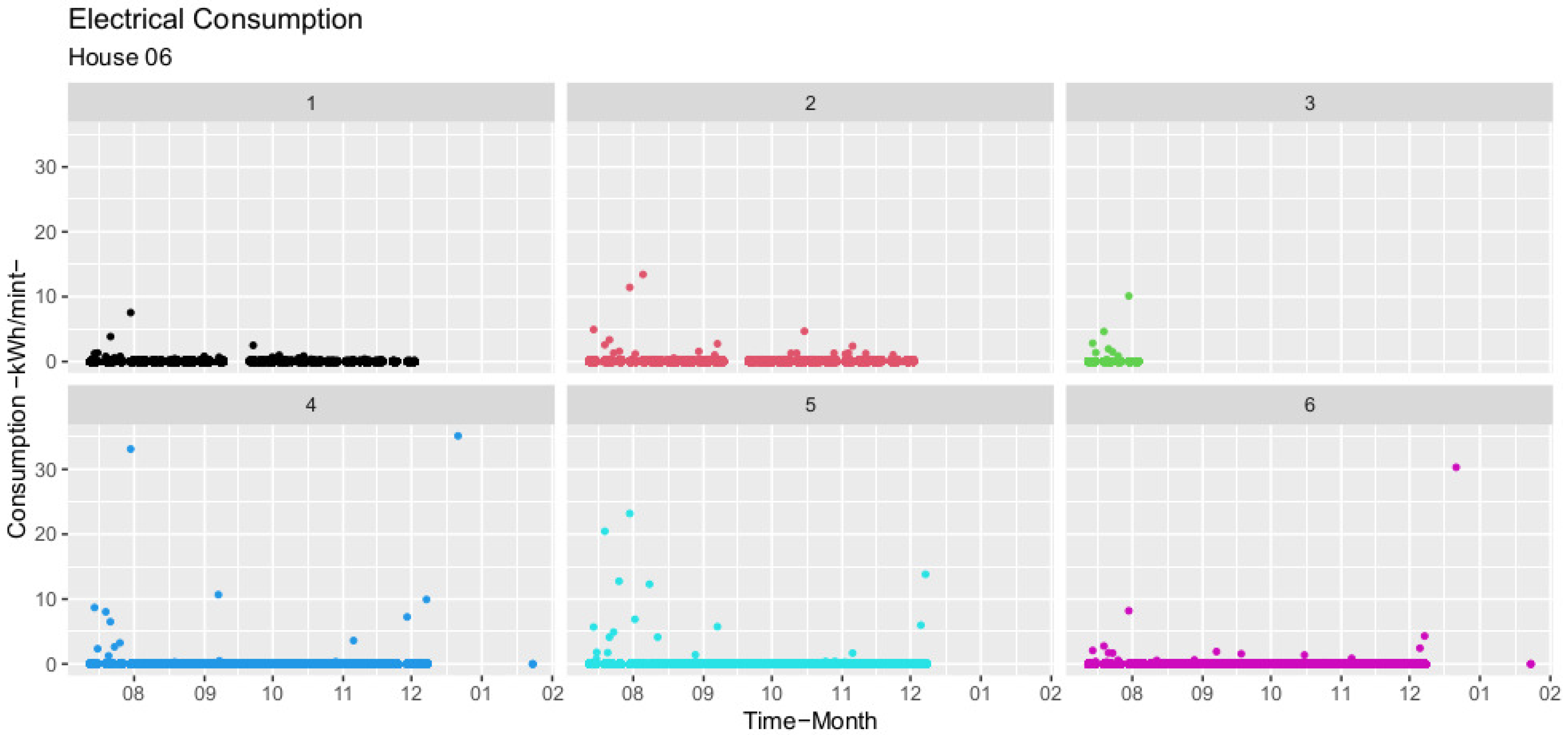
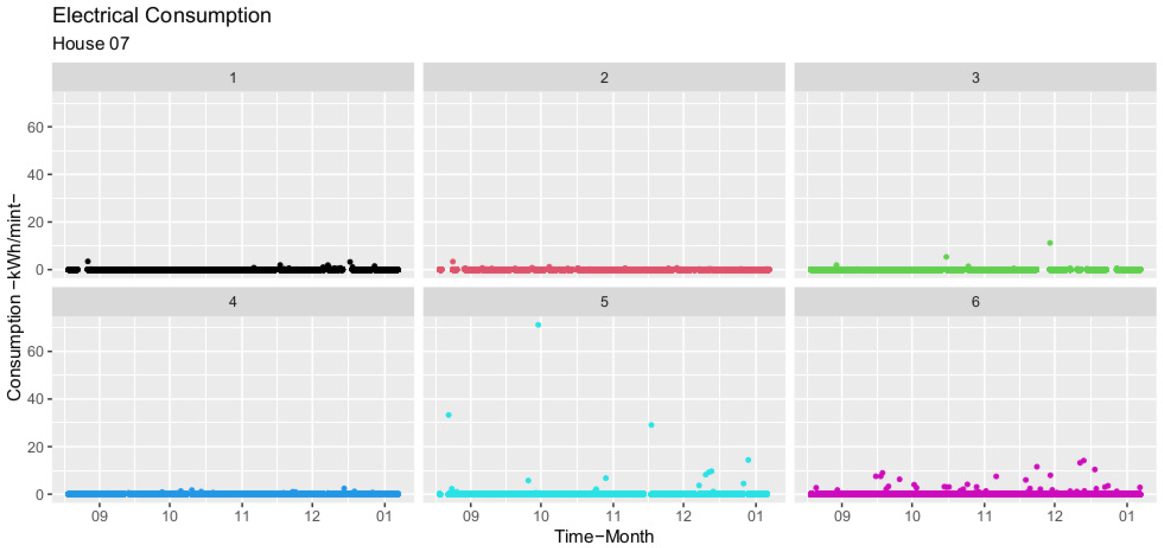
Appendix B. Energy Consumption Data Performance Graphs for Each House


Appendix C. Energy Consumption by m2 and per Capita
| House 1 | House 2 | House 3 | House 4 | House 5 | House 6 | House 7 | |
|---|---|---|---|---|---|---|---|
| month11 | 0.95 | −0.2 | 18.52 | −79,287.5 | −34,599.99 | 25,71.42 | −64.10 |
| month12 | 47.62 | −10.00 | −7.41 | −83,225.00 | 102,833.33 | 57,040.81 | −76.92 |
| device1 | 23.81 | 4.00 | −9.26 | 13,562.5 | −561,899.99 | −6010.20 | −153.84 |
| device2 | −2.38 | 10.00 | Ref | −83,481.25 | −502,566.66 | 2234.69 | −166.66 |
| device3 | −23.81 | 4.00 | −37.04 | Ref | −571,399.99 | Ref | −166.66 |
| device4 | −23.81 | 0.30 | −18.52 | −152,881.25 | −684,588.88 | 4663.26 | −153.84 |
| device5 | 23,81 | Ref | −37.04 | −50,268.75 | −570,366.66 | −2765.30 | −89.74 |
| device6 | Ref | N/A | −37.04 | −102,718.75 | Ref | N/A | Ref |
| mon | 0.24 | 0.40 | 3.70 | −8612.50 | −18,577.77 | 13,571.42 | −51.28 |
| tue | 47.62 | 0.30 | −3.70 | −64,375.00 | −61,344.44 | 11,408.16 | 5.12 |
| wed | 23.81 | 0.20 | 7.41 | −11,356.25 | 1388.88 | 6469.38 | −64.10 |
| thu | −9.52 | −1.00 | 7.41 | −17,025.00 | −21,166.66 | −8224.49 | 64.10 |
| fri | −7.14 | −0.30 | 18.52 | −75,150.00 | −78,444.44 | 7632.65 | 12.82 |
| sat | 71.43 | −0.10 | 18.52 | −2693.75 | −6855.55 | 9479.59 | −12.82 |
| holidays | −95.24 | −4.00 | −5.56 | 19,293.75 | −16,655.55 | −59,632.65 | −38.46 |
| House 1 | House 2 | House 3 | House 4 | House 5 | House 6 | House 7 | |
|---|---|---|---|---|---|---|---|
| h1 | −7.14 | −1.00 | 18.52 | 143.75 | 15,066.67 | −744.90 | −25.64 |
| h2 | −2.38 | −3.00 | −0.74 | 68.75 | 5788.89 | 4183.67 | −38.46 |
| h3 | −47.62 | −3.00 | −18.52 | −2362.50 | −103,211.11 | −857.14 | −25.64 |
| h4 | 95.24 | −4.00 | −18,52 | −1137.50 | 13,022.22 | −857.14 | −6.41 |
| h5 | −23.81 | −4.00 | −37.04 | 1962.50 | −15,955.56 | 1908.16 | −38.46 |
| h6 | −47.62 | −4.00 | −18.52 | 100.00 | −33,933.33 | −908.16 | −38.46 |
| h7 | −23.81 | −4.00 | −18.52 | 37.50 | −1033.33 | −1102.04 | 25.64 |
| h8 | −23.81 | −3.00 | −18.52 | −156.25 | 911.11 | −693.88 | −64.10 |
| h9 | −23.81 | −3.00 | −5.56 | 461,943.75 | 597,911.11 | 5214.29 | −25.64 |
| h10 | −23.81 | −2.00 | −18.52 | −16,268.75 | −133,222.22 | −12,183.67 | −25.64 |
| h11 | −23,81 | 1,00 | 5,56 | −12,975.00 | −15,155.56 | 4306,12 | −1,28 |
| h12 | −23,81 | 2,00 | −18,52 | −12,993.75 | −14,411.11 | 64,336.73 | −3,85 |
| h13 | −0.71 | 1.00 | −3.70 | −9393.75 | −23,411.11 | −2938.78 | 12.82 |
| h14 | −23.81 | 2.00 | −18.52 | −26,693.75 | −205,844.44 | 5857.14 | 2.56 |
| h15 | −23.81 | 3.00 | −7.41 | −13,268.75 | 62,233.33 | −612.24 | 3.85 |
| h16 | −23.81 | 1.00 | −18.52 | −12,168.75 | −9966.67 | 867.35 | −12.82 |
| h17 | −23.81 | 0.20 | 18.52 | −13,818.75 | −44,477.78 | −1122.45 | 12.82 |
| h18 | −9.52 | −0.30 | −5.56 | −11,918.75 | −22,933.33 | −1122.45 | 2.56 |
| h19 | −23.81 | 1,00 | −18.52 | −10,275.00 | 2288.89 | −1102.04 | 25.64 |
| h20 | 9.52 | 4.00 | 5.56 | −11,806.25 | −866.67 | −1357.14 | 64.10 |
| h21 | −47.62 | 10.00 | −18.52 | −11,762.50 | −10,677.78 | 1448.98 | 141.03 |
| h22 | −9.52 | 10.00 | −18.52 | −20,350.00 | −43,533.33 | −14,683.67 | 12.82 |
| h23 | −71.43 | 2.00 | −7.41 | −331.25 | −4588.89 | 3979.59 | 230.77 |
| House 1 | House 2 | House 3 | House 4 | House 5 | House 6 | House 7 | |
|---|---|---|---|---|---|---|---|
| D2 | −71.43 | −2.00 | 3.70 | 39,118.75 | 159,866.67 | −30,204.08 | −371.79 |
| D3 | −23.81 | −1.00 | 18.52 | 36,193.75 | −14,122.22 | −13,918.37 | −346.15 |
| D4 | −47.62 | −1.00 | −1.85 | 11,443.75 | −28,177.78 | −17,428.57 | −384.62 |
| D5 | −71.43 | −2.00 | 18.52 | 62,568.75 | 50,155.56 | −18,908.16 | −384.62 |
| D6 | −71.43 | −2.00 | −3.70 | −1100.00 | −15,844.44 | −775.51 | −346.15 |
| D7 | −23.81 | −2.00 | −5.56 | 18,843.75 | −18,166.67 | 2693.88 | −384.62 |
| D8 | −4.76 | −2.00 | −7.41 | −1931.25 | −17,344.44 | 877.55 | −333.33 |
| D9 | −71.43 | −4.00 | −1.85 | 42,668.75 | −13,866.67 | −3081.63 | −410.26 |
| D10 | −71.43 | −3.00 | 55.56 | 7543.75 | −8300.00 | 2561.22 | −358.97 |
| D11 | 190.48 | −2.00 | −0.37 | 12,700.00 | −5533.33 | 22,020.41 | −333.33 |
| D12 | −47.62 | −3.00 | 55.56 | 665,612.50 | 459,077.78 | −7265.31 | −371.79 |
| D13 | −71.43 | −4.00 | −9.26 | −35,387.50 | −41,644.44 | 5.10 | −333.33 |
| D14 | −47.62 | −2.00 | 3.70 | −16,881.25 | −28,522.22 | 9479.59 | −384.62 |
| D15 | −47.62 | −5.00 | −5.56 | 2.50 | 24,155.56 | −2397.96 | −307.69 |
| D16 | −71.43 | −5.00 | 18.52 | −9887.50 | −10,977.78 | −8397.96 | −307.69 |
| D17 | −47.62 | −4.00 | 37.04 | −37,750.00 | −59,144.44 | 3193.88 | −333.33 |
| D18 | −71.43 | −1.00 | 55.56 | −30,487.50 | −23,077.78 | 3479.9 | −358.97 |
| D19 | 23.81 | −2.00 | 18.52 | 26,325.00 | 30,333.33 | −6714.29 | −358.97 |
| D20 | −71.43 | −3.00 | 0.56 | −36,400.00 | −211,422.22 | 1000.00 | −320.51 |
| D21 | 95.24 | 0.00 | 37.04 | −44,600.00 | 99,011.11 | 158,744.90 | −384.62 |
| D22 | 47.62 | −4.00 | −1.85 | −1537.50 | 59,711.11 | −2224.49 | −358.97 |
| D23 | −71.43 | −2.00 | −3.70 | −15,000.00 | 36,877.78 | −4132.65 | −371.79 |
| D24 | −47.62 | −3.00 | 18.52 | −31,168.75 | −88,700.00 | 6020.41 | −346.15 |
| D25 | −9.52 | −0.50 | −18.52 | −30,525.00 | 98,411.11 | −5663.27 | −371.79 |
| D26 | −71.43 | −4.00 | 18.52 | 12,656.25 | 128,811.11 | −2908.16 | −384.62 |
| D27 | −47.62 | −5.00 | 74.07 | −32,031.25 | 57,744.44 | −40.82 | 12.82 |
| D28 | −23.81 | −2.00 | −1.85 | −28,250.00 | 13,466.66 | 11,336.73 | −358.97 |
| D29 | −23.81 | −3.00 | −5.56 | 4806.25 | 54,900.00 | −7336.73 | −333.33 |
| D30 | −71.43 | −4.00 | −1.85 | 58,968.75 | 21,455.56 | −3561.22 | −371.79 |
| D31 | 95.24 | −1.00 | 18.52 | −102,381.25 | −37,455.56 | 65,846.94 | −371.79 |
| House 1 | House 2 | House 3 | House 4 | House 5 | House 6 | House 7 | |
|---|---|---|---|---|---|---|---|
| month11 | 0.19 | −0.10 | 5.00 | −25,372.00 | −10,379.99 | 1260.00 | −16.66 |
| month12 | 10.00 | −5.00 | −2.00 | −26,632.00 | 30,849.99 | 27,950.00 | −20.00 |
| device1 | 5.00 | 2.00 | −2.50 | 4340.00 | −168,569.99 | −2945.00 | −40.00 |
| device2 | −0.49 | 5.00 | Ref | −26,714.00 | −150,769.99 | 1095.00 | −43.33 |
| device3 | −5.00 | 2.00 | −10.00 | Ref | −462.83 | Ref | −43.33 |
| device4 | −5.00 | 0.15 | −5.00 | −48,922.00 | −205,376.66 | 2285.00 | −40.00 |
| device5 | 5.00 | Ref | −10.00 | −16,086.00 | −171,109.99 | −1355.00 | −23.33 |
| device6 | Ref | N/A | −10.00 | −32,870.00 | Ref | N/A | Ref |
| mon | 0.05 | 0.20 | 0.99 | −2756.00 | −5573.33 | 6650.00 | −13.33 |
| tue | 10.00 | 0.15 | −0.99 | −20,600.00 | −18,403.33 | 5590.00 | 1.33 |
| wed | 5.00 | 0.10 | 2.00 | −3634.00 | 416.66 | 3170.00 | −16.66 |
| thu | −1.99 | −0.50 | 2.00 | −5448.00 | −6349.99 | −4030.00 | 16.66 |
| fri | −1.49 | −0.15 | 5.00 | −24,048.00 | −23,533.33 | 3740.00 | 3.33 |
| sat | 15.00 | −0.05 | 5.00 | −862.00 | −2056.66 | 4645.00 | −3.33 |
| holidays | −20.00 | −2.00 | −1.50 | 6174.00 | −4996.66 | −29,220.00 | −10.00 |
| House 1 | House 2 | House 3 | House 4 | House 5 | House 6 | House 7 | |
|---|---|---|---|---|---|---|---|
| h1 | −1.50 | −0.50 | 5.00 | 46.00 | 4520.00 | −365.00 | −6.67 |
| h2 | −0.50 | −1.50 | −0.20 | 22.00 | 1736.67 | 2050.00 | −10.00 |
| h3 | −10.00 | −1.50 | −5.00 | −756.00 | −30,963.33 | −420.00 | −6.67 |
| h4 | 20.00 | −2.00 | −5.00 | −364.00 | 3906.67 | −420.00 | −1.67 |
| h5 | −5.00 | −2.00 | −10.00 | 628.00 | −4786.67 | 935.00 | −10.00 |
| h6 | −10.00 | −2.00 | −5.00 | 32.00 | −10,180.00 | −445.00 | −10.00 |
| h7 | −5.00 | −2.00 | −5.00 | 12.00 | −310.00 | −540.00 | 6.67 |
| h8 | −5.00 | −1.50 | −5.00 | −50.00 | 273.33 | −340.00 | −16.67 |
| h9 | −5.00 | −1.50 | −1.50 | 147,822.00 | 179,373.33 | 2555.00 | −6.67 |
| h10 | −5.00 | −1.00 | −5.00 | −5206.00 | −39,966.67 | −5970.00 | −6.67 |
| h11 | −5.00 | 0.50 | 1.50 | −4152.00 | −4546.67 | 2110.00 | −0.33 |
| h12 | −5.00 | 1.00 | −5.00 | −4158.00 | −4323.33 | 31,525.00 | −1.00 |
| h13 | −0.15 | 0.50 | −1.00 | −3006.00 | −7023.33 | −1440.00 | 3.33 |
| h14 | −5.00 | 1.00 | −5.00 | −8542.00 | −61,753.33 | 2870.00 | 0.67 |
| h15 | −5.00 | 1.50 | −2.00 | −4.246.00 | 18,670.00 | −300.00 | 1.00 |
| h16 | −5.00 | 0.50 | −5.00 | −3894.00 | −2990.00 | 425.00 | −3.33 |
| h17 | −5.00 | 0.10 | 5.00 | −4422.00 | −13,343.33 | −550.00 | 3.33 |
| h18 | −2.00 | −0.15 | −1.50 | −3814.00 | −6880.00 | −550.00 | 0.67 |
| h19 | −5.00 | 0.50 | −5.00 | −3288.00 | 686.67 | −540.00 | 6.67 |
| h20 | 2.00 | 2.00 | 1.50 | −3778.00 | −260.00 | −665.00 | 16.67 |
| h21 | −10.00 | 5.00 | −5.00 | −3764.00 | −3203.33 | 710.00 | 36.67 |
| h22 | −2.00 | 5.00 | −5.00 | −6512.00 | −13,060.00 | −7195.00 | 3.33 |
| h23 | −15.00 | 1.00 | −2.00 | −106.00 | −1376.67 | 1950.00 | 60.00 |
| House 1 | House 2 | House 3 | House 4 | House 5 | House 6 | House 7 | |
|---|---|---|---|---|---|---|---|
| D2 | −15.00 | −1.00 | 1.00 | 12,518.00 | 47,960.00 | −14,800.00 | −96.67 |
| D3 | −5.00 | −0.50 | 5.00 | 11,582.00 | −4236.67 | −6820.00 | −90.00 |
| D4 | −10.00 | −0.50 | −0.50 | 3662.00 | −8453.33 | −8540.00 | −100.00 |
| D5 | −15.00 | −1.00 | 5.00 | 20,022.00 | 15,046.67 | −9265.00 | −100.00 |
| D6 | −15.00 | −1.00 | −1.00 | −352.00 | −4753.33 | −380.00 | −90.00 |
| D7 | −5.00 | −1.00 | −1.50 | 6030.00 | −5450.00 | 1320.00 | −100.00 |
| D8 | −1.00 | −1.00 | −2.00 | −618.00 | −5203.33 | 430.00 | −86.67 |
| D9 | −15.00 | −2.00 | −0.50 | 13,654.00 | −4160.00 | −1510.00 | −106.67 |
| D10 | −15.00 | −1.50 | 15.00 | 2414.00 | −2490.00 | 1255.00 | −93.33 |
| D11 | 40.00 | −1.00 | −0.10 | 4064.00 | −1660.00 | 10,790.00 | −86.67 |
| D12 | −10.00 | −1.50 | 15.00 | 212,996.00 | 137,723.33 | −3560.00 | −96.67 |
| D13 | −15.00 | −2.00 | −2.50 | −11,324.00 | −12,493.33 | 2.50 | −86.67 |
| D14 | −10.00 | −1.00 | 1.00 | −5402.00 | −8556.67 | 4645.00 | −100.00 |
| D15 | −10.00 | −2.50 | −1.50 | 0.80 | 7246.67 | −1175.00 | −80.00 |
| D16 | −15.00 | −2.50 | 5.00 | −3164.00 | −3293.33 | −4115.00 | −80.00 |
| D17 | −10.00 | −2.00 | 10.00 | −12,080.00 | −17,743.33 | 1565.00 | −86.67 |
| D18 | −15.00 | −0.50 | 15.00 | −9756.00 | −6923.33 | 1705.00 | −93.33 |
| D19 | 5.00 | −1.00 | 5.00 | 8424.00 | 9100.00 | −3290.00 | −93.33 |
| D20 | −15.00 | −1.50 | 0.15 | −11,648.00 | −63,426.67 | 490.00 | −83.33 |
| D21 | 20.00 | 0.00 | 10.00 | −14,272.00 | 29,703.33 | 77,785.00 | −100.00 |
| D22 | 10.00 | −2.00 | −0.50 | −492.00 | 17,913.33 | −1090.00 | −93.33 |
| D23 | −15.00 | −1.00 | −1.00 | −4800.00 | 11,063.33 | −2025.00 | −96.67 |
| D24 | −10.00 | −1.50 | 5.00 | −9974.00 | −26,610.00 | 2950.00 | −90.00 |
| D25 | −2.00 | −0.25 | −5.00 | −9768.00 | 29,523.33 | −2775.00 | −96.67 |
| D26 | −15.00 | −2.00 | 5.00 | 4050.00 | 38,643.33 | −1425.00 | −100.00 |
| D27 | −10.00 | −2.50 | 20.00 | −10,250.00 | 17,323.33 | −20.00 | 3.33 |
| D28 | −5.00 | −1.00 | −0.50 | −9040.00 | 4040.00 | 5555.00 | −93.33 |
| D29 | −5.00 | −1.50 | −1.50 | 1538.00 | 16,470.00 | −3595.00 | −86.67 |
| D30 | −15.00 | −2.00 | −0.50 | 18,870.00 | 6436.67 | −1745.00 | −96.67 |
| D31 | 20.00 | −0.50 | 5.00 | −32,762.00 | −11,236.67 | 32,265.00 | −96.67 |
| House 1 | House 2 | House 3 | House 4 | House 5 | House 6 | House 7 | |
|---|---|---|---|---|---|---|---|
| month8 | N/A | −10.00 | −18.51 | −393.75 | −3.33 | 2683.67 | 346.15 |
| month9 | −23.81 | −10.00 | −18.51 | −881.25 | −77.77 | 25,122.44 | 282.05 |
| month10 | −47.62 | −0.30 | −18.51 | 1331.25 | −0.22 | 26,795.91 | 128.20 |
| month11 | −47.62 | −1.00 | −0.18 | −756.25 | −66.66 | 27,469.38 | 64.10 |
| month12 | N/A | 10.00 | −37.03 | −500.00 | −133.33 | 94,744.90 | N/A |
| device1 | 142.86 | −50.00 | −5.55 | −1550.00 | −188.88 | −7336.73 | −217.94 |
| device2 | 23.81 | −50.00 | Ref | −1881.25 | −255.55 | −2795.91 | −282.05 |
| device3 | −23.81 | −50.00 | −18.51 | Ref | −288.88 | −4010.20 | −243.58 |
| device4 | −23.81 | −50.00 | −18.51 | −1718.75 | −288.88 | 1928.57 | −269.23 |
| device5 | 23.81 | Ref | −18.51 | −1681.25 | −144.44 | −3071.42 | −179.48 |
| device6 | Ref | −50.00 | −18.51 | −1618.75 | Ref | Ref | Ref |
| mon | −0.24 | 2.00 | −1.85 | 325.00 | −22.22 | 2602.04 | 217.94 |
| tue | 23.81 | 1.00 | −5.55 | 75.00 | 22.22 | −2632.65 | 51.28 |
| wed | 9.52 | −1.00 | −1.85 | −31.25 | 33.33 | −1377.55 | 76.92 |
| thu | −7.14 | −3.00 | −5.55 | 131.25 | 33.33 | −2795.91 | 102.56 |
| fri | −2.38 | −2.00 | −1.85 | 1618.75 | −2.22 | −122.44 | 38.46 |
| sat | 23.81 | 1.00 | −9.25 | 37.5 | 22.22 | −2500.00 | 115.38 |
| holidays | −95.24 | 3.00 | −5.55 | 125.00 | 33.33 | −31,428.57 | 397.43 |
| House 1 | House 2 | House 3 | House 4 | House 5 | House 6 | House 7 | |
|---|---|---|---|---|---|---|---|
| h1 | 0.00 | −1.00 | 7.41 | 218.75 | −22.22 | −193.88 | −25.64 |
| h2 | 2.38 | −4.00 | −18.52 | −250.00 | −22.22 | −16,408.16 | −38.46 |
| h3 | −23.81 | −4.00 | −18.52 | −312.50 | 66.67 | 5306.12 | 6.41 |
| h4 | 95.24 | −4.00 | −18.52 | −306.25 | 155.56 | −20.41 | −12.82 |
| h5 | −9.52 | −4.00 | −18.52 | 43.75 | −55.56 | 795.92 | 25.64 |
| h6 | −23.81 | −4.00 | −18.52 | −237,50 | −33.33 | −112.24 | −38.46 |
| h7 | −23.81 | −4.00 | −18.52 | −206.25 | −44.44 | 357.14 | −38.46 |
| h8 | −23.81 | −3.00 | −18.52 | −106.25 | −155.56 | 459.18 | 12.82 |
| h9 | −23.81 | −2.00 | 18.52 | 350.00 | 88.89 | 3571.43 | −2.56 |
| h10 | −23.81 | −1.00 | 37.04 | −12.50 | 4.44 | −14,602.04 | 12.82 |
| h11 | −23.81 | 5.00 | 9.26 | 31.25 | 55.56 | 1714.29 | 25.64 |
| h12 | −23.81 | 30.00 | 1.85 | 168.75 | 33.33 | 51,857.14 | 25.64 |
| h13 | 23.81 | 10.00 | 18.52 | 25.00 | −22.22 | 1693.88 | 51.28 |
| h14 | −23.81 | 10.00 | −7.41 | 12.50 | 33.33 | 4142.86 | 38.46 |
| h15 | −23.81 | 10.00 | −7.41 | −481.25 | 111.11 | −51.02 | 38.46 |
| h16 | −9.52 | 10.00 | −1.85 | 131.25 | −22.22 | −1142.86 | 25.64 |
| h17 | −23.81 | 10.00 | 18.52 | −87.50 | −77.78 | −1081.63 | 38.46 |
| h18 | −7.14 | −10.00 | 5.56 | 75.00 | −44.44 | −510.20 | 89.74 |
| h19 | −7.14 | 30.00 | 5.56 | −487.50 | −44.44 | −1581.63 | 38.46 |
| h20 | 9.52 | 40.00 | 7.41 | −112.50 | −11.11 | 867.35 | 89.74 |
| h21 | −23.81 | 40.00 | 18.52 | −100.00 | 11.11 | 714.29 | 153.85 |
| h22 | −2.38 | 20.00 | 18.52 | −106.25 | 33.33 | −8397.96 | 782.05 |
| h23 | −71.43 | 10.00 | −3.70 | 7281.25 | −55.56 | 469.39 | 179.49 |
| holidays | −95.24 | 3.00 | −5.56 | 125.00 | 33.33 | −31,428.57 | 397.44 |
| dst | −4.76 | −10.00 | 1.85 | 337.50 | 100.00 | −22,346.94 | 243.59 |
| House 1 | House 2 | House 3 | House 4 | House 5 | House 6 | House 7 | |
|---|---|---|---|---|---|---|---|
| D2 | −47.62 | 0.30 | 7.41 | 106.25 | 44.44 | −20,857.14 | −51.28 |
| D3 | −23.81 | −2.00 | 3.70 | −218.75 | 111.11 | −20.41 | −12.82 |
| D4 | −47.62 | 0.20 | 9.26 | 387.50 | 333.33 | −3755.10 | −128.21 |
| D5 | −47.62 | −4.00 | 5.56 | 0.63 | 44.44 | −2561.22 | −320.51 |
| D6 | −47.62 | 1.00 | −1.85 | −181.25 | −22.22 | 7714.29 | −205.13 |
| D7 | −47.62 | 0.00 | 18.52 | 425.00 | 177.78 | 8867.35 | −76.92 |
| D8 | −23.81 | 4.00 | −7.41 | 312.50 | 22.22 | −1193.88 | −205.13 |
| D9 | −47.62 | 10.00 | −1.85 | −31.25 | 22.22 | 14,510.20 | −128.21 |
| D10 | −71.43 | 10.00 | 18.52 | 156.25 | −11.11 | 12,826.53 | −102.56 |
| D11 | 190.48 | 4.00 | −3.70 | 475.00 | −33.33 | 17,102.04 | −256.41 |
| D12 | −23.81 | 10.00 | 18.52 | −93.75 | 133.33 | 16,071.43 | −38.46 |
| D13 | −47.62 | 10.00 | 18.52 | −331.25 | −55.56 | 9316.33 | −128.21 |
| D14 | −47.62 | 10.00 | 0.19 | 7556.25 | −22.22 | 14,122.45 | −102.56 |
| D15 | −23.81 | 10.00 | 5.56 | −318.75 | −22.22 | 21,295.92 | −115.38 |
| D16 | −47.62 | −2.00 | 18.52 | −156.25 | −33.33 | 11,030.61 | −115.38 |
| D17 | −47.62 | −4.00 | −1.85 | −306.25 | −66.67 | 18,969.39 | −89.74 |
| D18 | −47.62 | −2.00 | 18.52 | 206.25 | −22.22 | 18,306.12 | −115.38 |
| D19 | 0.48 | 20.00 | 7.41 | −337.50 | 22.22 | 17,377.55 | 692.31 |
| D20 | −47.62 | 3.00 | −5.56 | −293.75 | 88.89 | 8612.24 | −153.85 |
| D21 | 95.24 | 10.00 | 3.70 | 150.00 | 66.67 | 115,010.20 | −179.49 |
| D22 | 47.62 | 2.00 | −5.56 | 200.00 | 122.22 | 13,591.84 | −76.92 |
| D23 | −47.62 | 4.00 | −5.56 | 175.00 | −22.22 | 15,091.84 | −128.21 |
| D24 | −47.62 | 2.00 | 18.52 | 256.25 | −44.44 | 14,091.84 | 6.41 |
| D25 | −23.81 | 3.00 | 9.26 | 81.25 | −44.44 | 11,275.51 | −217.95 |
| D26 | −23.81 | 4.00 | 18.52 | −656.25 | 77.78 | 15,704.08 | −76.92 |
| D27 | −23.81 | −20.00 | 18.52 | −287.50 | −3.33 | 13,132.65 | 230.77 |
| D28 | −23.81 | 10.00 | 18.52 | −568.75 | −22.22 | 14,163.27 | −51.28 |
| D29 | −23.81 | 5.00 | 0.56 | 131.25 | 22.22 | 10,183.67 | 2.56 |
| D30 | −23.81 | 3.00 | 1.85 | −456.25 | −33.33 | 14,122.45 | −166.67 |
| D31 | 71.43 | −10.00 | −1.85 | −806.25 | −55.56 | 21,867.35 | −243.59 |
| House 1 | House 2 | House 3 | House 4 | House 5 | House 6 | House 7 | |
|---|---|---|---|---|---|---|---|
| month8 | N/A | −5.00 | −5.00 | −126.00 | −1.00 | 1315.00 | 90.00 |
| month9 | −5.00 | −5.00 | −5.00 | −282.00 | −23.33 | 12,310.00 | 73.33 |
| month10 | −10.00 | −0.15 | −5.00 | 426.00 | −0.06 | 13,130.00 | 33.33 |
| month11 | −10.00 | −0.50 | −0.05 | −242.00 | −20.00 | 13,460.00 | 16.66 |
| month12 | N/A | 5.00 | −10.00 | −160.00 | −40.00 | 46,425.00 | N/A |
| device1 | 30.00 | −25.00 | −1.50 | −496.00 | −56.66 | −3595.00 | −56.66 |
| device2 | 5.00 | −25.00 | Ref | −602.00 | −76.66 | −1370.00 | −73.33 |
| device3 | −5.00 | −25.00 | −5.00 | Ref | −86.66 | −1965.00 | −63.33 |
| device4 | −5.00 | −25.00 | −5.00 | −550.00 | −86.66 | 945.00 | −70.00 |
| device5 | 5.00 | Ref | −5.00 | −538.00 | −43.33 | −1505.00 | −46.66 |
| device6 | Ref | −25.00 | −5.00 | −518.00 | Ref | Ref | Ref |
| mon | −0.05 | 1.00 | −0.50 | 104.00 | −6.66 | 1275.00 | 56.66 |
| tue | 5.00 | 0.50 | −1.50 | 24.00 | 6.66 | −1290.00 | 13.33 |
| wed | 1.99 | −0.50 | −0.50 | −10.00 | 10.00 | −675.00 | 20.00 |
| thu | −1.49 | −1.50 | −1.50 | 42.00 | 10.00 | −1370.00 | 26.66 |
| fri | −0.49 | −1.00 | −0.50 | 518.00 | −0.66 | −60.00 | 10.00 |
| sat | 5.00 | 0.50 | −2.50 | 12.00 | 6.66 | −1225.00 | 30.00 |
| holidays | −20.00 | 1.50 | −1.50 | 40.00 | 10.00 | −15,400.00 | 103.33 |
| House 1 | House 2 | House 3 | House 4 | House 5 | House 6 | House 7 | |
|---|---|---|---|---|---|---|---|
| h1 | 0.00 | −0.50 | 2.00 | 70.00 | −6.67 | −95.00 | −6.67 |
| h2 | 0.50 | −2.00 | −5.00 | −80.00 | −6.67 | −8040.00 | −10.00 |
| h3 | −5.00 | −2.00 | −5.00 | −100.00 | 20.00 | 2600.00 | 1.67 |
| h4 | 20.00 | −2.00 | −5.00 | −98.00 | 46.67 | −10.00 | −3.33 |
| h5 | −2.00 | −2.00 | −5.00 | 14.00 | −16.67 | 390.00 | 6.67 |
| h6 | −5.00 | −2.00 | −5.00 | −76.00 | −10.00 | −55.00 | −10.00 |
| h7 | −5.00 | −2.00 | −5.00 | −66.00 | −13.33 | 175.00 | −10.00 |
| h8 | −5.00 | −1.50 | −5.00 | −34.00 | −46.67 | 225.00 | 3.33 |
| h9 | −5.00 | −1.00 | 5.00 | 112.00 | 26.67 | 1750.00 | −0.67 |
| h10 | −5.00 | −0.50 | 10.00 | −4.00 | 1.33 | −7155.00 | 3.33 |
| h11 | −5.00 | 2.50 | 2.50 | 10.00 | 16.67 | 840.00 | 6.67 |
| h12 | −5.00 | 15.00 | 0.50 | 54.00 | 10.00 | 25,410.00 | 6.67 |
| h13 | 5.00 | 5.00 | 5.00 | 8.00 | −6.67 | 830.00 | 13.33 |
| h14 | −5.00 | 5.00 | −2.00 | 4.00 | 10.00 | 2030.00 | 10.00 |
| h15 | −5.00 | 5.00 | −2.00 | −154.00 | 33.33 | −25.00 | 10.00 |
| h16 | −2.00 | 5.00 | −0.50 | 42.00 | −6.67 | −560.00 | 6.67 |
| h17 | −5.00 | 5.00 | 5.00 | −28.00 | −23.33 | −530.00 | 10.00 |
| h18 | −1.50 | −5.00 | 1.50 | 24.00 | −13.33 | −250.00 | 23.33 |
| h19 | −1.50 | 15.00 | 1.50 | −156.00 | −13.33 | −775.00 | 10.00 |
| h20 | 2.00 | 20.00 | 2.00 | −36.00 | −3.33 | 425.00 | 23.33 |
| h21 | −5.00 | 20.00 | 5.00 | −32.00 | 3.33 | 350.00 | 40.00 |
| h22 | −0.50 | 10.00 | 5.00 | −34.00 | 10.00 | −4115.00 | 203.33 |
| h23 | −15.00 | 5.00 | −1.00 | 2330.00 | −16.67 | 230.00 | 46.67 |
| holidays | −20.00 | 1.50 | −1.50 | 40.00 | 10.00 | −15,400.00 | 103.33 |
| dst | −1.00 | −5.00 | 0.50 | 108.00 | 30.00 | −10,950.00 | 63.33 |
| House 1 | House 2 | House 3 | House 4 | House 5 | House 6 | House 7 | |
|---|---|---|---|---|---|---|---|
| D2 | −10.00 | 0.15 | 2.00 | 34.00 | 13.33 | −10,220.00 | −13.33 |
| D3 | −5.00 | −1.00 | 1.00 | −70.00 | 33.33 | −10.00 | −3.33 |
| D4 | −10.00 | 0.10 | 2.50 | 124.00 | 100.00 | −1840.00 | −33.33 |
| D5 | −10.00 | −2.00 | 1.50 | 0.20 | 13.33 | −1255.00 | −83.33 |
| D6 | −10.00 | 0.50 | −0.50 | −58.00 | −6.67 | 3780.00 | −53.33 |
| D7 | −10.00 | 0.00 | 5.00 | 136.00 | 53.33 | 4345.00 | −20.00 |
| D8 | −5.00 | 2.00 | −2.00 | 100.00 | 6.67 | −585.00 | −53.33 |
| D9 | −10.00 | 5.00 | −0.50 | −10.00 | 6.67 | 7110.00 | −33.33 |
| D10 | −15.00 | 5.00 | 5.00 | 50.00 | −3.33 | 6285.00 | −26.67 |
| D11 | 40.00 | 2.00 | −1.00 | 152.00 | −10.00 | 8380.00 | −66.67 |
| D12 | −5.00 | 5.00 | 5.00 | −30.00 | 40.00 | 7875.00 | −10.00 |
| D13 | −10.00 | 5.00 | 5.00 | −106.00 | −16.67 | 4565.00 | −33.33 |
| D14 | −10.00 | 5.00 | 0.05 | 2418.00 | −6.67 | 6920.00 | −26.67 |
| D15 | −5.00 | 5.00 | 1.50 | −102.00 | −6.67 | 10,435.00 | −30.00 |
| D16 | −10.00 | −1.00 | 5.00 | −50.00 | −10.00 | 5405.00 | −30.00 |
| D17 | −10.00 | −2.00 | −0.50 | −98.00 | −20.00 | 9295.00 | −23.33 |
| D18 | −10.00 | −1.00 | 5.00 | 66.00 | −6.67 | 8970.00 | −30.00 |
| D19 | 0.10 | 10.00 | 2.00 | −108.00 | 6.67 | 8515.00 | 180.00 |
| D20 | −10.00 | 1.50 | −1.50 | −94.00 | 26.67 | 4220.00 | −40.00 |
| D21 | 20.00 | 5.00 | 1.00 | 48.00 | 20.00 | 56,355.00 | −46.67 |
| D22 | 10.00 | 1.00 | −1.50 | 64.00 | 36.67 | 6660.00 | −20.00 |
| D23 | −10.00 | 2.00 | −1.50 | 56.00 | −6.67 | 7395.00 | −33.33 |
| D24 | −10.00 | 1.00 | 5.00 | 82.00 | −13.33 | 6905.00 | 1.67 |
| D25 | −5.00 | 1.50 | 2.50 | 26.00 | −13.33 | 5525.00 | −56.67 |
| D26 | −5.00 | 2.00 | 5.00 | −210.00 | 23.33 | 7695.00 | −20.00 |
| D27 | −5.00 | −10.00 | 5.00 | −92.00 | −1.00 | 6435.00 | 60.00 |
| D28 | −5.00 | 5.00 | 5.00 | −182.00 | −6.67 | 6940.00 | −13.33 |
| D29 | −5.00 | 2.50 | 0.15 | 42.00 | 6.67 | 4990.00 | 0.67 |
| D30 | −5.00 | 1.50 | 0.50 | −146.00 | −10.00 | 6920.00 | −43.33 |
| D31 | 15.00 | −5.00 | −0.50 | −258.00 | −16.67 | 10,715.00 | −63.33 |
References
- McLoughlin, F.; Duffy, A.; Conlon, M. Characterising domestic electricity consumption patterns by dwelling and occupant socio-economic variables: An Irish case study. Energy Build. 2012, 48, 240–248. [Google Scholar] [CrossRef]
- Yohanis, Y.G.; Mondol, J.D.; Wright, A.; Norton, B. Real-life energy use in the UK: How occupancy and dwelling characteristics affect domestic electricity use. Energy Build. 2008, 40, 1053–1059. [Google Scholar] [CrossRef]
- Stegner, C.; Glaß, O.; Beikircher, T. Comparing smart metered, residential power demand with standard load profiles. Sustain. Energy Grids Netw. 2019, 20, 100248. [Google Scholar] [CrossRef]
- Fischer, D.; Härtl, A.; Wille-Haussmann, B. Model for electric load profiles with high time resolution for German households. Energy Build. 2015, 92, 170–179. [Google Scholar] [CrossRef]
- Jeong, H.C.; Jang, M.; Kim, T.; Joo, S.-K. Clustering of Load Profiles of Residential Customers Using Extreme Points and Demographic Characteristics. Electronics 2021, 10, 290. [Google Scholar] [CrossRef]
- Hayn, M.; Bertsch, V.; Fichtner, W. Electricity load profiles in Europe: The importance of household segmentation. Energy Res. Soc. Sci. 2014, 3, 30–45. [Google Scholar] [CrossRef]
- Andersen, F.; Gunkel, P.; Jacobsen, H.; Kitzing, L. Residential electricity consumption and household characteristics: An econometric analysis of Danish smart-meter data. Energy Econ. 2021, 100, 105341. [Google Scholar] [CrossRef]
- Kang, J.; Reiner, D.M. What is the effect of weather on household electricity consumption? Empirical evidence from Ireland. Energy Econ. 2022, 111, 106023. [Google Scholar] [CrossRef]
- Ghanem, D.; Smith, A. What are the benefits of high-frequency data for fixed effects panel models? J. Assoc. Environ. Resour. Econ. 2021, 8, 199–234. [Google Scholar]
- Dyson, M.E.; Borgeson, S.D.; Tabone, M.D.; Callaway, D.S. Using smart meter data to estimate demand response potential, with application to solar energy integration. Energy Policy 2014, 73, 607–619. [Google Scholar] [CrossRef]
- Gao, Y.; Fang, C.; Zhang, J. A Spatial Analysis of Smart Meter Adoptions: Empirical Evidence from the U.S. Data. Sustainability 2022, 14, 1126. [Google Scholar] [CrossRef]
- Köhler, S.; Rongstock, R.; Hein, M.; Eicker, U. Similarity measures and comparison methods for residential electricity load profiles. Energy Build. 2022, 271, 112327. [Google Scholar] [CrossRef]
- Belton, C.A.; Lunn, P.D. Smart choices? An experimental study of smart meters and time-of-use tariffs in Ireland. Energy Policy 2020, 140, 111243. [Google Scholar] [CrossRef]
- Flor, M.; Herraiz, S.; Contreras, I. Definition of Residential Power Load Profiles Clusters Using Machine Learning and Spatial Analysis. Energies 2021, 14, 6565. [Google Scholar] [CrossRef]
- Anvari, M.; Proedrou, E.; Schäfer, B.; Beck, C.; Kantz, H.; Timme, M. Data-driven load profiles and the dynamics of residential electricity consumption. Nat. Commun. 2022, 13, 4593. [Google Scholar] [CrossRef] [PubMed]
- Leslie, G.W.; Pourkhanali, A.; Roger, G. Electricity consumption, ethnic origin and religion. Energy Econ. 2022, 114, 106249. [Google Scholar] [CrossRef]
- Dergiades, T.; Tsoulfidis, L. Estimating residential demand for electricity in the United States, 1965–2006. Energy Econ. 2008, 30, 2722–2730. [Google Scholar] [CrossRef]
- Moral-Carcedo, J.; Vicéns-Otero, J. Modelling the non-linear response of Spanish electricity demand to temperature variations. Energy Econ. 2005, 27, 477–494. [Google Scholar] [CrossRef]
- Miller, J.I.; Nam, K. Modeling peak electricity demand: A semiparametric approach using weather-driven cross-temperature response functions. Energy Econ. 2022, 114, 106291. [Google Scholar] [CrossRef]
- Ivanov, C.; Getachew, L.; Fenrick, S.A.; Vittetoe, B. Enabling technologies and energy savings: The case of EnergyWise Smart Meter Pilot of Connexus Energy. Util. Policy 2013, 26, 76–84. [Google Scholar] [CrossRef]
- Roach, C. Estimating electricity impact profiles for building characteristics using smart meter data and mixed models. Energy Build. 2020, 211, 109686. [Google Scholar] [CrossRef]
- Weigert, A.; Hopf, K.; Günther, S.A.; Staake, T. Heat pump inspections result in large energy savings when a pre-selection of households is performed: A promising use case of smart meter data. Energy Policy 2022, 169, 113156. [Google Scholar] [CrossRef]
- Bardazzi, R.; Pazienza, M.G. When I was your age: Generational effects on long-run residential energy consumption in Italy. Energy Res. Soc. Sci. 2020, 70, 101611. [Google Scholar] [CrossRef]
- Glasgo, B.; Hendrickson, C.; Azevedo, I.M. Using advanced metering infrastructure to characterize residential energy use. Electr. J. 2017, 30, 64–70. [Google Scholar] [CrossRef]
- Sims-Williams, F. A review of British Standard 6871: 1987. J. Sterile Serv. Manag. 1988, 5, 19. [Google Scholar]
- United States Secretary of Transportation. The Year-Round Daylight Saving Time Study; Report 1; Department of Transportation: Washington, DC, USA, 1974. [Google Scholar]
- Kotchen, M.J.; Grant, L.E. Does Daylight Saving Time Save Energy? Evidence from a Natural Experiment in Indiana. Rev. Econ. Stat. 2011, 93, 1172–1185. [Google Scholar] [CrossRef]
- Kellogg, R.; Wolff, H. Daylight time and energy: Evidence from an Australian experiment. J. Environ. Econ. Manag. 2008, 56, 207–220. [Google Scholar] [CrossRef]
- Krarti, M.; Hajiah, A. Analysis of impact of daylight time savings on energy use of buildings in Kuwait. Energy Policy 2011, 39, 2319–2329. [Google Scholar] [CrossRef]
- Mirza, F.M.; Bergland, O. The impact of daylight saving time on electricity consumption: Evidence from southern Norway and Sweden. Energy Policy 2011, 39, 3558–3571. [Google Scholar] [CrossRef]
- Ahuja, D.R.; SenGupta, D. Year-round daylight saving time will save more energy in India than corresponding DST or time zones. Energy Policy 2012, 42, 657–669. [Google Scholar] [CrossRef]
- Verdejo, H.; Becker, C.; Echiburu, D.; Escudero, W.; Fucks, E. Impact of daylight saving time on the Chilean residential consumption. Energy Policy 2016, 88, 456–464. [Google Scholar] [CrossRef]
- Rivers, N. Does Daylight Savings Time Save Energy? Evidence from Ontario. Environ. Resour. Econ. 2018, 70, 517–543. [Google Scholar] [CrossRef]
- Choi, S.; Pellen, A.; Masson, V. How does daylight saving time affect electricity demand? An answer using aggregate data from a natural experiment in Western Australia. Energy Econ. 2017, 66, 247–260. [Google Scholar] [CrossRef]
- Hancevic, P.; Margulis, D. Horario de verano y consumo de electricidad: El caso de Argentina. Trimest. Econ. 2018, 85, 515–542. [Google Scholar] [CrossRef]
- Flores, D.; Luna, E.M. An econometric evaluation of daylight saving time in Mexico. Energy 2019, 187, 116124. [Google Scholar] [CrossRef]
- Giacomelli-Sobrinho, V.; Cudlínová, E.; Buchtele, R.; Sagapova, N. The tropical twilight of Daylight-Saving Time (DST): Enlightening energy savings from electricity markets across Brazilian regions. Energy Sustain. Dev. 2022, 67, 81–92. [Google Scholar] [CrossRef]
- Kudela, P.; Havranek, T.; Herman, D.; Irsova, Z. Does daylight saving time save electricity? Evidence from Slovakia. Energy Policy 2020, 137, 111146. [Google Scholar] [CrossRef]
- Shaffer, B. Location matters: Daylight saving time and electricity demand. Can. J. Econ. 2019, 52, 1374–1400. [Google Scholar] [CrossRef]
- López, M. Daylight effect on the electricity demand in Spain and assessment of Daylight Saving Time policies. Energy Policy 2020, 140, 111419. [Google Scholar] [CrossRef]
- Guven, C.; Yuan, H.; Zhang, Q.; Aksakalli, V. When does daylight saving time save electricity? Weather and air-conditioning. Energy Econ. 2021, 98, 105216. [Google Scholar] [CrossRef]
- Küfeoğlu, S.; Üçler, Ş.; Eskicioğlu, F.; Öztürk, E.B.; Chen, H. Daylight Saving Time policy and energy consumption. Energy Rep. 2021, 7, 5013–5025. [Google Scholar] [CrossRef]
- Stock, J.; Watson, M. Introduction to Econometrics, 3rd ed.; Addison Wesley Longman: London, UK, 2011. [Google Scholar]
- Wooldridge, J.M. Econometric Analysis of Cross Section and Panel Data; MIT Press: Cambridge, MA, USA, 2010. [Google Scholar]
- Almasri, R.A.; Alshitawi, M. Electricity consumption indicators and energy efficiency in residential buildings in GCC countries: Extensive review. Energy Build. 2022, 255, 111664. [Google Scholar] [CrossRef]

| N° House | Commune | Device 1 | Device 2 | Device 3 | Device 4 | Device 5 | Device 6 |
|---|---|---|---|---|---|---|---|
| House 1 | Nunoa | Electric kettle | Television 40″ | Television 42″ | Notebook | Lamp | Refrigerator |
| House 2 | Cerro Navia | Computer | Television 55″ | Refrigerator | Television 43″ | Electric heater | Microwave |
| House 3 | Estación Central | Refrigerator | Wahing machine | Oven | Computer | Television 55″ | Electric heater |
| House 4 | La Reina | Television | Refrigerator | Electric water heater | Computer | Kettle | Television 32″ |
| House 5 | Macul | Television 41″ | Vertical freezer | Television 50″ | Washing machine | Refrigerator | Cooler |
| House 6 | Providencia | Oven | Electric kettle | Power strip | Television 55″ | Refrigerator | Router |
| House 7 | Macul | Refrigerator | Oven | Notebook | Microwave | PC Tower | Television 55″ |
| Name of Variable (s) | Description |
|---|---|
| Dummys for each hour of the day | |
| Dummys for each month of the year (Aug–Dec) | |
| Dummys for each device analyzed inside the house | |
| – | Dummys for each day of the month (2–31) |
| Dummy for each day of the week (Mon–Sat) | |
| Dummy for holiday = 1 | |
| Dummy for Daylight Saving Time = 1 |
| House 1 | House 2 | House 3 | House 4 | House 5 | House 6 | House 7 | |
|---|---|---|---|---|---|---|---|
| month11 | 0.00004 | −0.00002 *** | 0.001 *** | −12.686 *** | −3.114 *** | 0.252 *** | −0.005 *** |
| (0.00004) | (0.00001) | (0.0002) | (0.281) | (0.235) | (0.023) | (0.0004) | |
| month12 | 0.002 *** | −0.001 *** | −0.0004 * | −13.316 *** | 9.255 *** | 5.590 *** | −0.006 *** |
| (0.0001) | (0.00004) | (0.0002) | (0.363) | (0.412) | (0.070) | (0.001) | |
| device1 | 0.001 *** | 0.0004 *** | −0.0005 * | 2.170 *** | −50.571 *** | −0.589 *** | −0.012 *** |
| (0.0002) | (0.00001) | (0.0003) | (0.371) | (0.779) | (0.035) | (0.001) | |
| device2 | −0.0001 ** | 0.001 *** | Ref | −13.357 *** | −45.231 *** | 0.219 *** | −0.013 *** |
| (0.0001) | (0.00001) | (0.321) | (0.687) | (0.038) | (0.001) | ||
| device3 | −0.001 *** | 0.0004 *** | −0.002 *** | Ref | −51.426 *** | Ref | −0.013 *** |
| (0.0001) | (0.00001) | (0.0002) | (0.718) | (0.001) | |||
| device4 | −0.001 *** | 0.00003 ** | −0.001 ** | −24.461 *** | −61.613 *** | 0.457 *** | −0.012 *** |
| (0.0001) | (0.00001) | (0.0003) | (0.352) | (0.818) | (0.030) | (0.001) | |
| device5 | 0.001 *** | Ref | −0.002 *** | −8.043 *** | −51.333 *** | −0.271 *** | −0.007 *** |
| (0.0001) | (0.0002) | (0.283) | (0.762) | (0.027) | (0.001) | ||
| device6 | Ref | N/A | −0.002 *** | −16.435 *** | Ref | N/A | Ref |
| (0.0002) | (0.284) | ||||||
| mon | 0.00001 | 0.00004 *** | 0.0002 | −1.378 *** | −1.672 *** | 1.330 *** | −0.004 *** |
| (0.0001) | (0.00002) | (0.0001) | (0.474) | (0.551) | (0.038) | (0.001) | |
| tue | 0.002 *** | 0.00003 * | −0.0002 | −10.300 *** | −5.521 *** | 1.118 *** | 0.0004 |
| (0.0003) | (0.00002) | (0.0002) | (0.491) | (0.527) | (0.039) | (0.0003) | |
| wed | 0.001 *** | 0.00002 * | 0.0004 | −1.817 *** | 0.125 | 0.634 *** | −0.005 *** |
| (0.0001) | (0.00001) | (0.0002) | (0.408) | (0.486) | (0.034) | (0.001) | |
| thu | −0.0004 *** | −0.0001 *** | 0.0004 *** | −2.724 *** | −1.905 *** | −0.806 *** | 0.005 *** |
| (0.0001) | (0.00001) | (0.0001) | (0.389) | (0.475) | (0.050) | (0.001) | |
| fri | −0.0003 *** | −0.00003 | 0.001 *** | −12.024 *** | −7.060 *** | 0.748 *** | 0.001 *** |
| (0.0001) | (0.00002) | (0.0002) | (0.512) | (0.574) | (0.036) | (0.0005) | |
| sat | 0.003 *** | −0.00001 | 0.001 ** | −0.431 | −0.617 | 0.929 *** | −0.001 * |
| (0.0002) | (0.00001) | (0.0002) | (0.451) | (0.565) | (0.033) | (0.0004) | |
| holidays | −0.004 *** | −0.0004 *** | −0.0003 ** | 3.087 *** | −1.499 ** | −5.844 *** | −0.003 *** |
| (0.0003) | (0.00002) | (0.0001) | (0.404) | (0.586) | (0.107) | (0.001) | |
| Constant | 0.002 *** | 0.001 *** | 0.001 *** | 21.487 *** | 48.485 *** | −0.880 *** | 0.043 *** |
| (0.0003) | (0.00005) | (0.0004) | (0.731) | (1.048) | (0.092) | (0.005) | |
| Observations | 746,259 | 603,075 | 728,203 | 718,326 | 679,465 | 538,216 | 735,553 |
| 0.033 | 0.032 | 0.002 | 0.797 | 0.510 | 0.826 | 0.016 | |
| Adjusted | 0.033 | 0.032 | 0.002 | 0.797 | 0.510 | 0.826 | 0.016 |
| Residual Std. Error | 0.017 (df = 746,191) | 0.002 (df = 603,008) | 0.034 (df = 728,135) | 31.749 (df = 718,258) | 34.593 (df = 679,397) | 2.764 (df = 538,149) | 0.081 (df = 735,485) |
| F Statistic | 378.505 *** (df = 67; 746,191) | 299.483 *** (df = 66; 603,008) | 20.106 *** (df = 67; 728,135) | 42,075.420 *** (df = 67; 718,258) | 10,554.980 *** (df = 67; 679,397) | 38,638.270 *** (df = 66; 538,149) | 182.887 *** (df = 67; 735,485) |
| House 1 | House 2 | House 3 | House 4 | House 5 | House 6 | House 7 | |
|---|---|---|---|---|---|---|---|
| month8 | N/A | −0.001 *** | −0.001 *** | −0.063 *** | −0.0003 | 0.263 *** | 0.027 *** |
| (0.0001) | (0.0001) | (0.003) | (0.001) | (0.022) | (0.002) | ||
| month9 | −0.001 *** | −0.001 *** | −0.001 *** | −0.141 *** | −0.007 *** | 2.462 *** | 0.022 *** |
| (0.0001) | (0.0001) | (0.0002) | (0.011) | (0.002) | (0.047) | (0.001) | |
| month10 | −0.002 *** | −0.00003 | −0.001 *** | 0.213 *** | −0.00002 | 2.626 *** | 0.010 *** |
| (0.0001) | (0.0001) | (0.0002) | (0.028) | (0.004) | (0.052) | (0.001) | |
| month11 | −0.002 *** | −0.0001 | −0.00001 | −0.121 *** | −0.006 *** | 2.692 *** | 0.005 *** |
| (0.0001) | (0.0001) | (0.0002) | (0.008) | (0.002) | (0.051) | (0.0004) | |
| month12 | N/A | 0.001 *** | −0.002 *** | −0.080 *** | −0.012 *** | 9.285 *** | N/A |
| (0.0001) | (0.0002) | (0.007) | (0.003) | (0.093) | |||
| device1 | 0.006 *** | −0.005 *** | −0.0003 | −0.248 *** | −0.017 *** | −0.719 *** | −0.017 *** |
| (0.0001) | (0.0002) | (0.0002) | (0.017) | (0.002) | (0.016) | (0.001) | |
| device2 | 0.001 *** | −0.005 *** | Ref | −0.301 *** | −0.023 *** | −0.274 *** | −0.022 *** |
| (0.00004) | (0.0002) | (0.021) | (0.002) | (0.023) | (0.001) | ||
| device3 | −0.001 *** | −0.005 *** | −0.001 *** | Ref | −0.026 *** | −0.393 *** | −0.019 *** |
| (0.00003) | (0.0002) | (0.0001) | (0.002) | (0.069) | (0.001) | ||
| device4 | −0.001 *** | −0.005 *** | −0.001 *** | −0.275 *** | −0.026 *** | 0.189 *** | −0.021 *** |
| (0.00003) | (0.0002) | (0.0002) | (0.018) | (0.002) | (0.019) | (0.001) | |
| device5 | 0.001 *** | Ref | −0.001 *** | −0.269 *** | −0.013 *** | −0.301 *** | −0.014 *** |
| (0.0001) | (0.0002) | (0.017) | (0.002) | (0.015) | (0.001) | ||
| device6 | Ref | −0.005 *** | −0.001 *** | −0.259 *** | Ref | Ref | Ref |
| (0.0002) | (0.0002) | (0.018) | |||||
| mon | −0.00001 | 0.0002 ** | −0.0001 | 0.052 *** | −0.002 *** | 0.255 *** | 0.017 *** |
| (0.00005) | (0.0001) | (0.0002) | (0.007) | (0.0005) | (0.020) | (0.001) | |
| tue | 0.001 *** | 0.0001 | −0.0003 *** | 0.012 ** | 0.002 | −0.258 *** | 0.004 *** |
| (0.0001) | (0.0001) | (0.0001) | (0.005) | (0.002) | (0.022) | (0.0005) | |
| wed | 0.0004 *** | −0.0001 | −0.0001 | −0.005 | 0.003 ** | −0.135 *** | 0.006 *** |
| (0.0001) | (0.0001) | (0.0001) | (0.003) | (0.001) | (0.022) | (0.001) | |
| thu | −0.0003 *** | −0.0003 *** | −0.0003 *** | 0.021 *** | 0.003 *** | −0.274 *** | 0.008 *** |
| (0.00003) | (0.0001) | (0.0001) | (0.008) | (0.001) | (0.021) | (0.001) | |
| fri | −0.0001 | −0.0002 *** | −0.0001 | 0.259 *** | −0.0002 | −0.012 | 0.003 *** |
| (0.00004) | (0.0001) | (0.0001) | (0.027) | (0.001) | (0.019) | (0.001) | |
| sat | 0.001 *** | 0.0001 | −0.0005 *** | 0.006 * | 0.002 ** | −0.245 *** | 0.009 *** |
| (0.0001) | (0.0001) | (0.0001) | (0.004) | (0.001) | (0.022) | (0.001) | |
| holidays | −0.004 | 0.0003 ** | −0.0003 *** | 0.020 *** | 0.003 * | −3.080 *** | 0.031 *** |
| (0.0003) | (0.0001) | (0.0001) | (0.006) | (0.002) | (0.047) | (0.002) | |
| Constant | 0.003 *** | 0.006 *** | 0.002 *** | 0.191 *** | 0.024 *** | −1.481 *** | −0.013 *** |
| (0.0004) | (0.0002) | (0.0002) | (0.010) | (0.002) | (0.064) | (0.003) | |
| Observations | 1,633,802 | 1,783,481 | 1,749,531 | 1,672,655 | 1,648,740 | 1,304,140 | 1,653,857 |
| 0.067 | 0.024 | 0.001 | 0.030 | 0.002 | 0.657 | 0.036 | |
| Adjusted | 0.067 | 0.024 | 0.0005 | 0.030 | 0.002 | 0.656 | 0.036 |
| Residual Std. Error | 0.011 (df = 1,633,732) | 0.014 (df = 1,783,409) | 0.043 (df = 1,749,459) | 1.787 (df = 1,672,583) | 0.330 (df = 1,648,668) | 2.533 (df = 1,304,068) | 0.107 (df = 1,653,786) |
| F Statistic | 1706.848 *** (df = 69; 1,633,732) | 614.282 *** (df = 71; 1,783,409) | 12.813 *** (df = 71; 1,749,459) | 732.879 *** (df = 71; 1,672,583) | 38.180 *** (df = 71; 1,648,668) | 35,103.650 *** (df = 71; 1,304,068) | 875.066 *** (df = 70; 1,653,786) |
| House 1 | House 2 | House 3 | House 4 | House 5 | House 6 | House 7 | |
|---|---|---|---|---|---|---|---|
| Model 1 | 3.3 | 3.2 | 0.2 | 79.7 | 51.0 | 82.6 | 1.6 |
| Model 2 | 6.7 | 2.4 | 0.1 | 3.0 | 0.2 | 65.7 | 3.6 |
Disclaimer/Publisher’s Note: The statements, opinions and data contained in all publications are solely those of the individual author(s) and contributor(s) and not of MDPI and/or the editor(s). MDPI and/or the editor(s) disclaim responsibility for any injury to people or property resulting from any ideas, methods, instructions or products referred to in the content. |
© 2023 by the authors. Licensee MDPI, Basel, Switzerland. This article is an open access article distributed under the terms and conditions of the Creative Commons Attribution (CC BY) license (https://creativecommons.org/licenses/by/4.0/).
Share and Cite
Verdejo, H.; Fucks Jara, E.; Castillo, T.; Becker, C.; Vergara, D.; Sebastian, R.; Guzmán, G.; Tobar, F.; Zolezzi, J. Analysis and Modeling of Residential Energy Consumption Profiles Using Device-Level Data: A Case Study of Homes Located in Santiago de Chile. Sustainability 2024, 16, 255. https://doi.org/10.3390/su16010255
Verdejo H, Fucks Jara E, Castillo T, Becker C, Vergara D, Sebastian R, Guzmán G, Tobar F, Zolezzi J. Analysis and Modeling of Residential Energy Consumption Profiles Using Device-Level Data: A Case Study of Homes Located in Santiago de Chile. Sustainability. 2024; 16(1):255. https://doi.org/10.3390/su16010255
Chicago/Turabian StyleVerdejo, Humberto, Emiliano Fucks Jara, Tomas Castillo, Cristhian Becker, Diego Vergara, Rafael Sebastian, Guillermo Guzmán, Francisco Tobar, and Juan Zolezzi. 2024. "Analysis and Modeling of Residential Energy Consumption Profiles Using Device-Level Data: A Case Study of Homes Located in Santiago de Chile" Sustainability 16, no. 1: 255. https://doi.org/10.3390/su16010255
APA StyleVerdejo, H., Fucks Jara, E., Castillo, T., Becker, C., Vergara, D., Sebastian, R., Guzmán, G., Tobar, F., & Zolezzi, J. (2024). Analysis and Modeling of Residential Energy Consumption Profiles Using Device-Level Data: A Case Study of Homes Located in Santiago de Chile. Sustainability, 16(1), 255. https://doi.org/10.3390/su16010255