
Models and Methods for Quantifying the Environmental, Economic, and Social Benefits and Challenges of Green Infrastructure: A Critical Review


Abstract
1. Introduction
2. Methodology
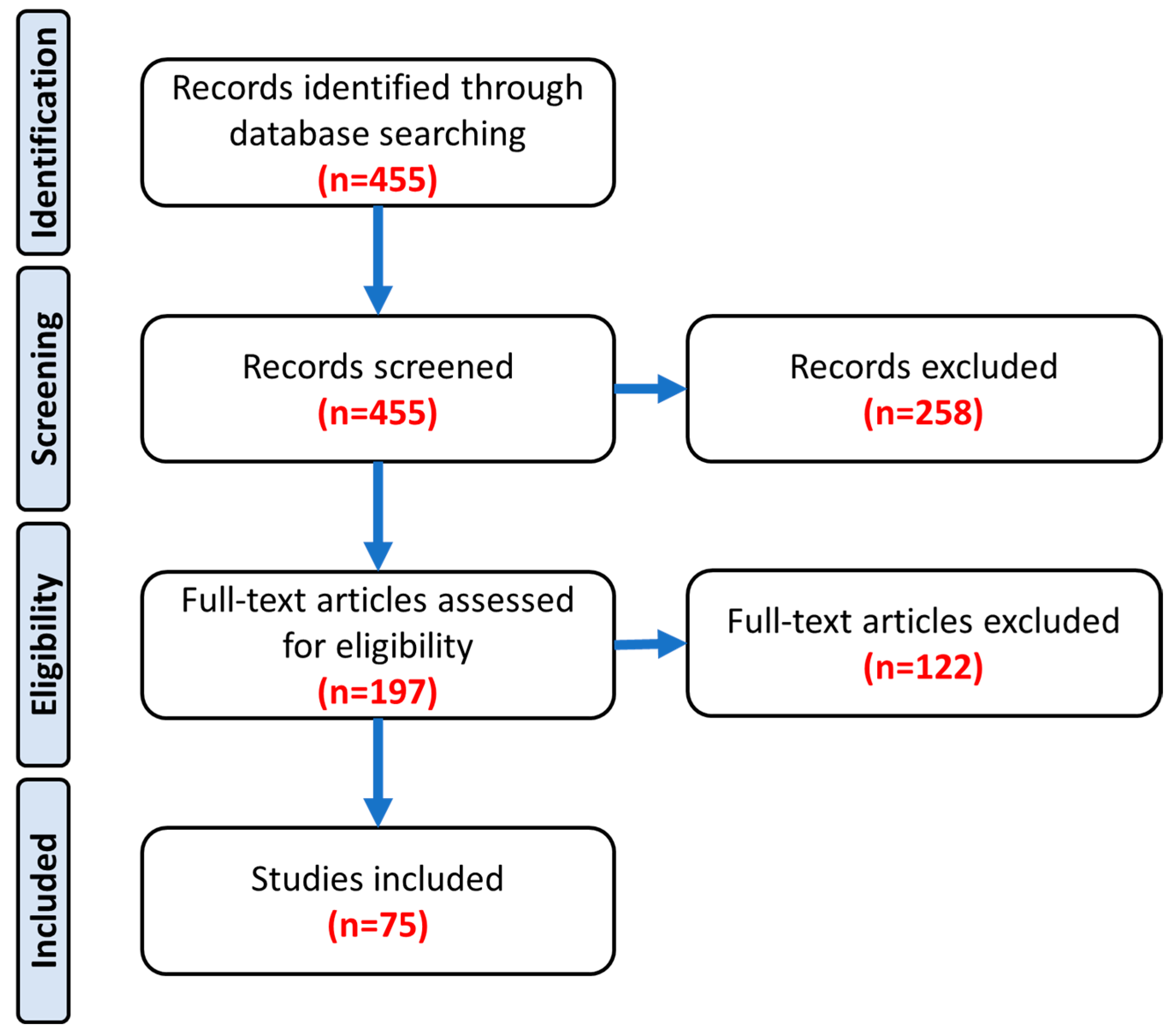
2.1. Identification of Articles
2.2. Screening of Articles
2.3. Eligibility of Articles
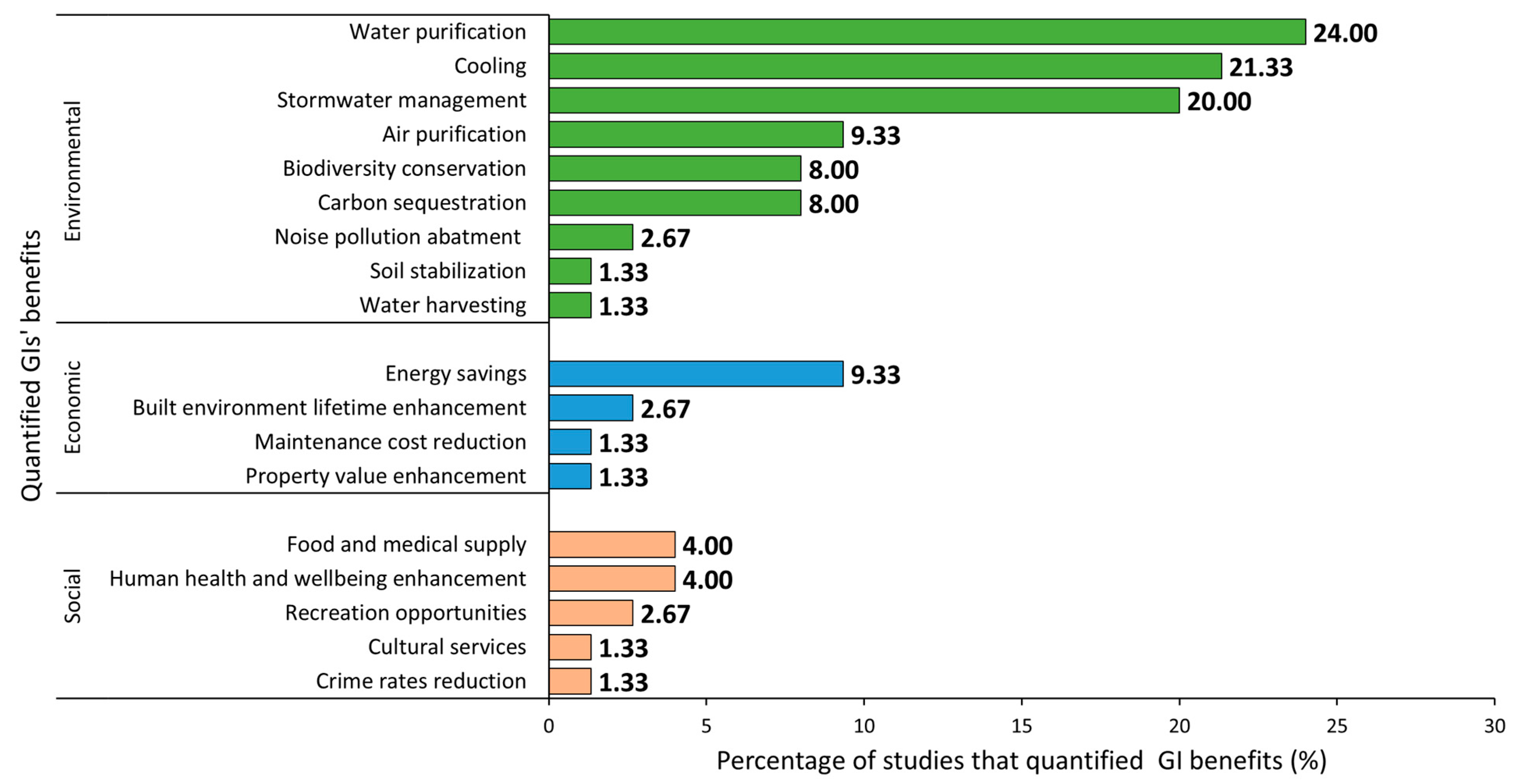
3. Results
3.1. Environmental Benefits
3.1.1. Air Purification
3.1.2. Carbon Sequestration
3.1.3. Cooling
3.1.4. Stormwater Management
3.1.5. Water Purification
3.1.6. Water Harvesting
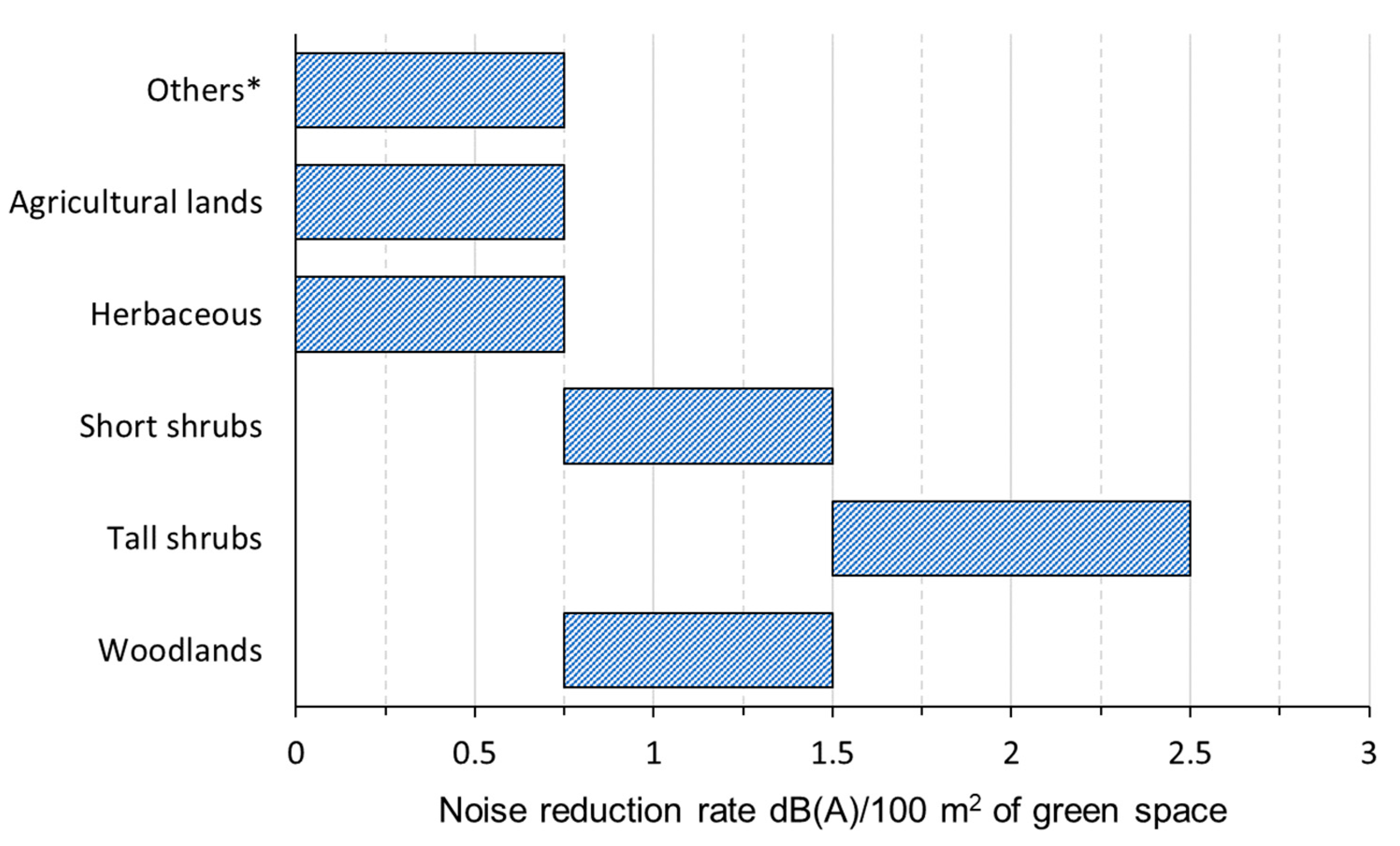
3.1.7. Noise Pollution Reduction
3.1.8. Biodiversity Conservation
3.1.9. Soil Stabilization
3.2. Economic Benefits
3.2.1. Energy Saving
3.2.2. Property Value Enhancement
3.2.3. Built Environment Lifetime Enhancement
3.2.4. Maintenance Cost Reduction
3.3. Social Benefits
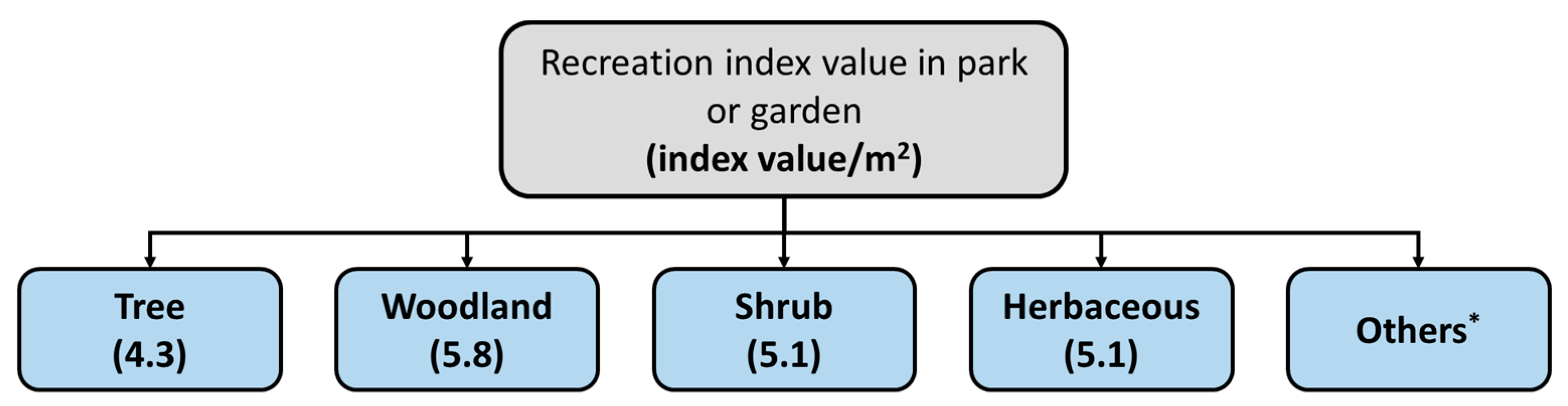
3.3.1. Recreation Opportunities
3.3.2. Human Health and Well-Being Enhancement
3.3.3. Crime Rate Reduction
3.3.4. Food and Medical Supply
3.3.5. Cultural Services
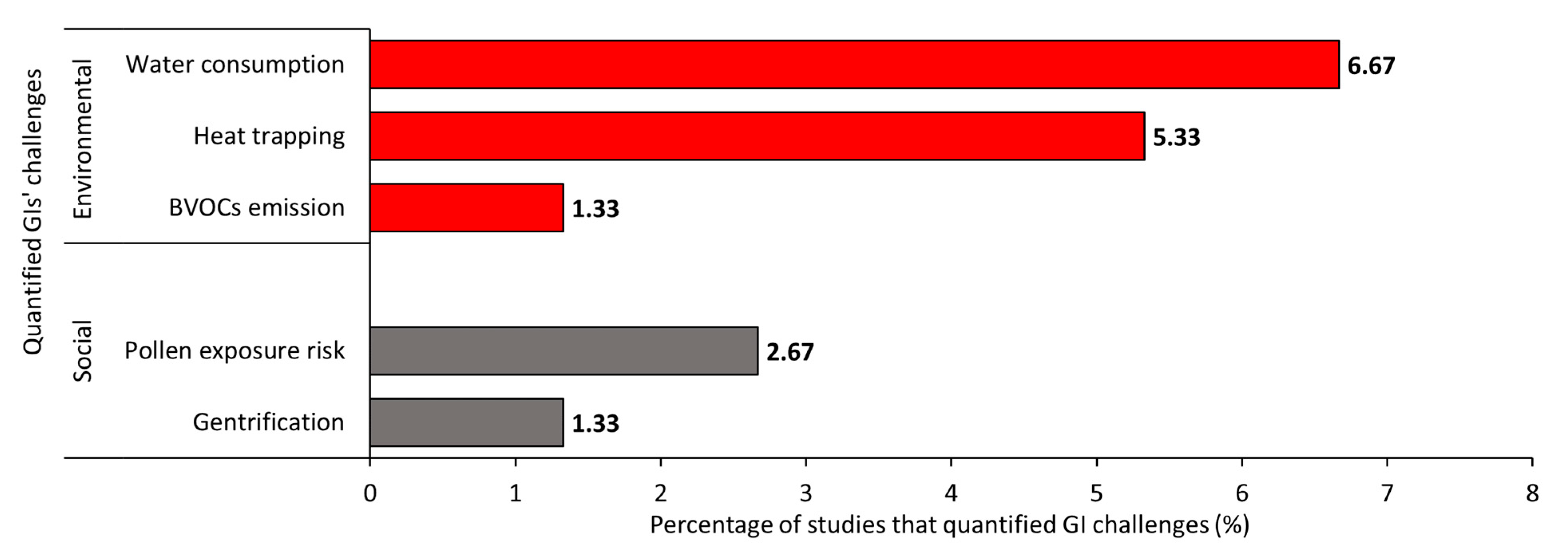
3.4. Environmental Challenges
3.4.1. BVOCs Emission
3.4.2. Heat-Trapping
3.4.3. Water Consumption
3.5. Social Challenges
3.5.1. Gentrification
3.5.2. Pollen Exposure Risk
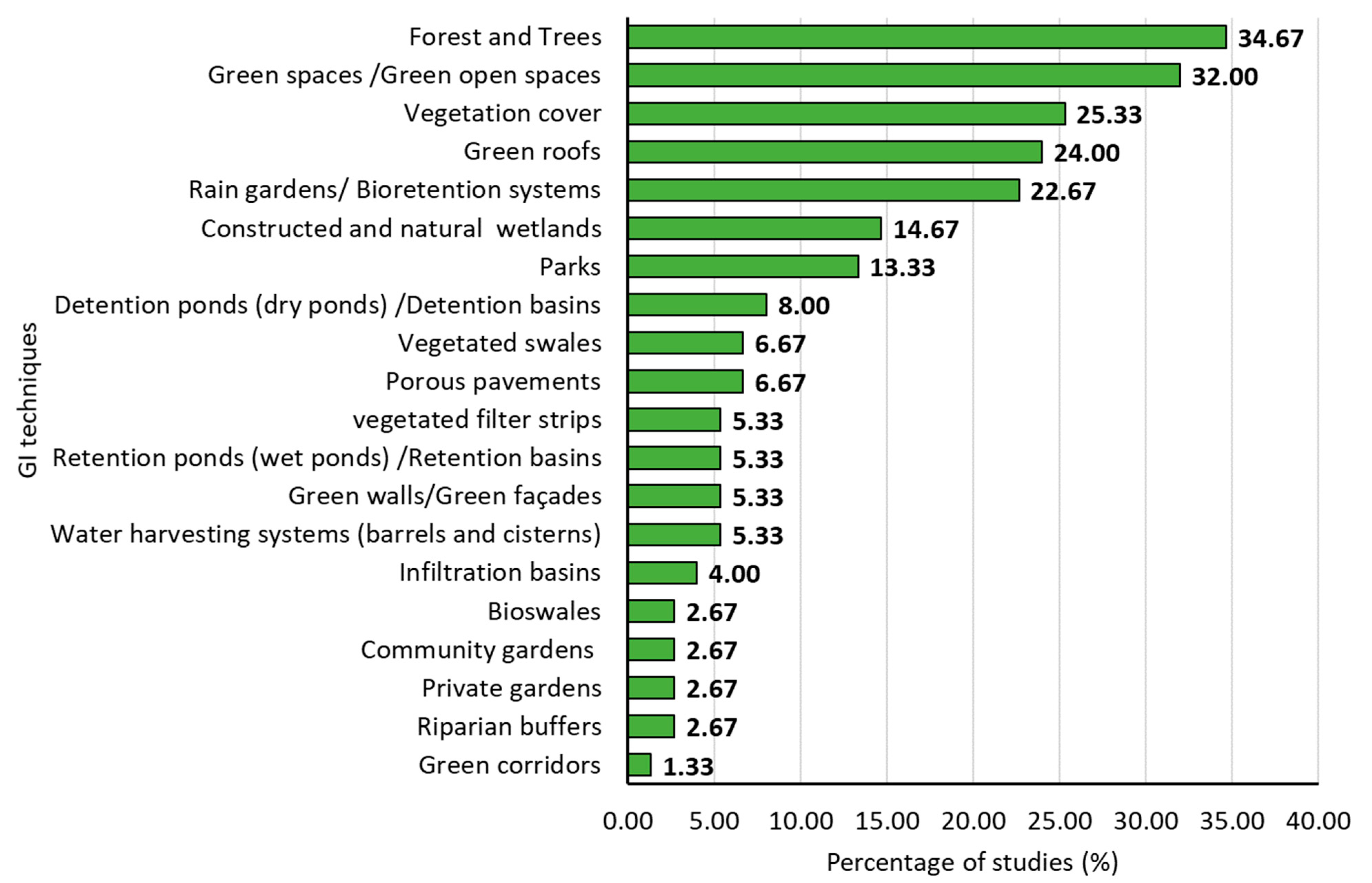
3.6. Summary of Benefits and Challenges Based on GI Techniques
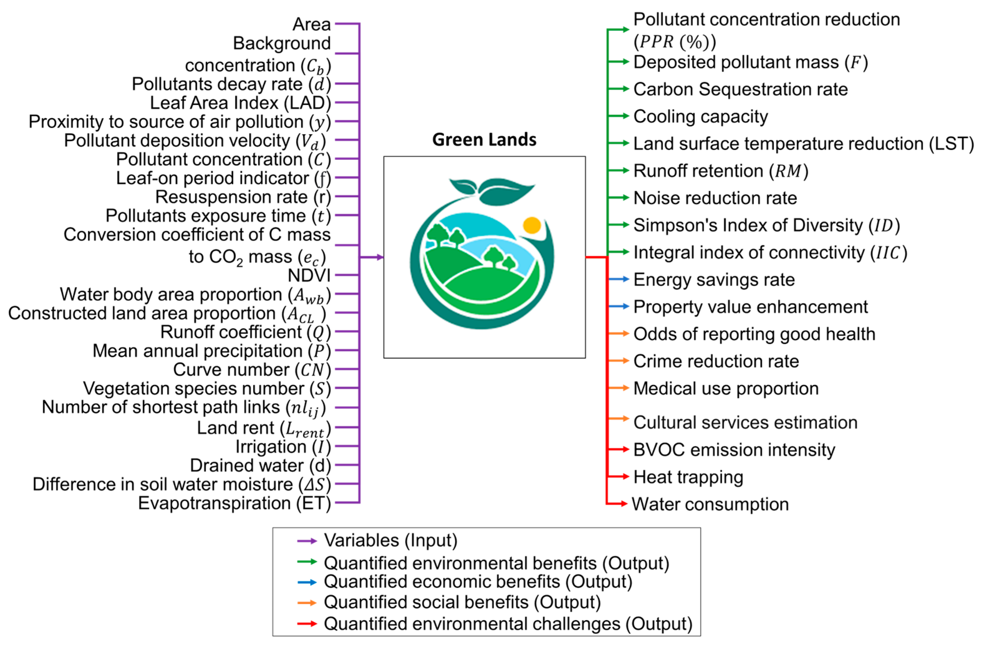
3.6.1. Green Lands
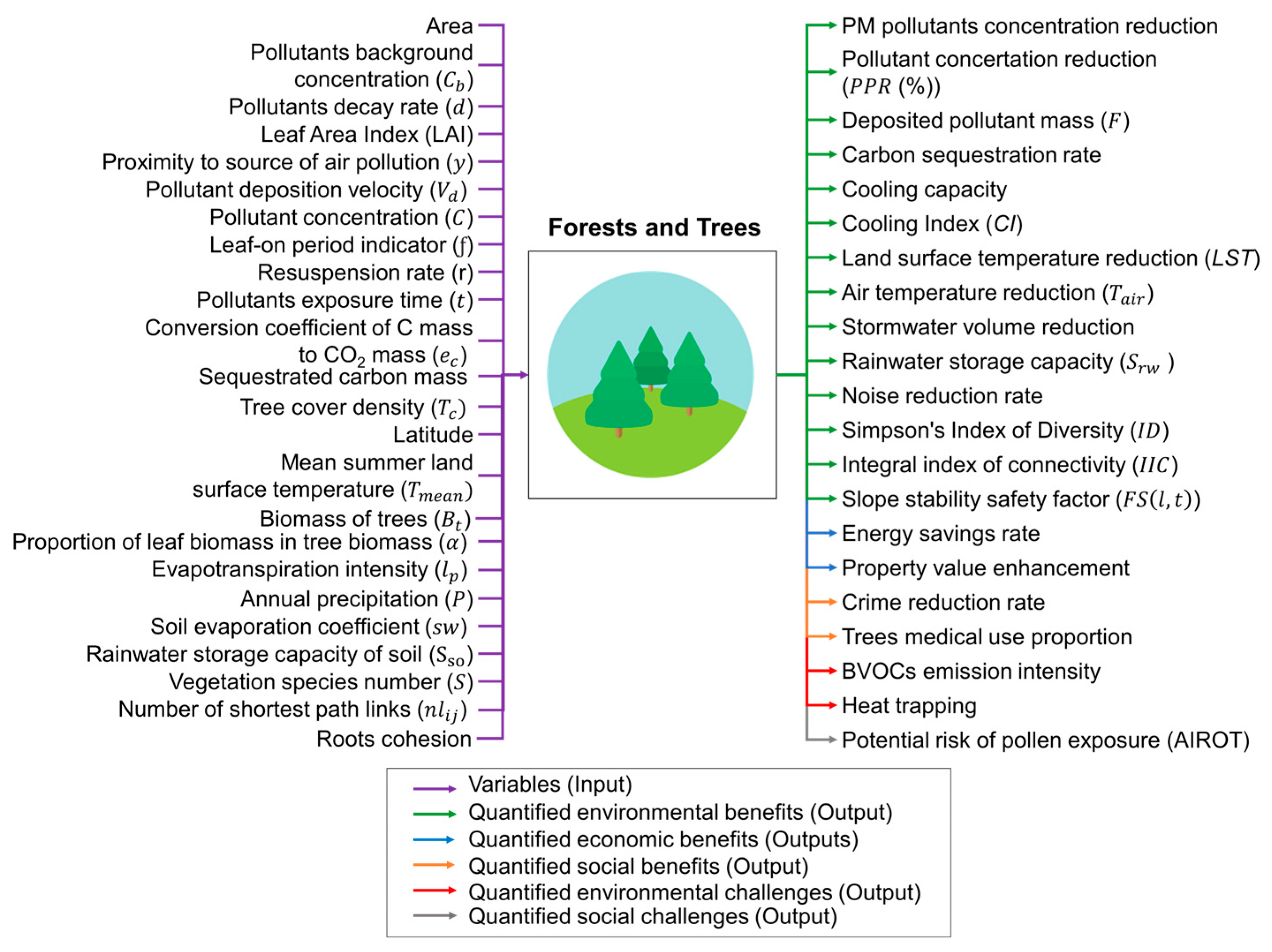
3.6.2. Forests and Trees
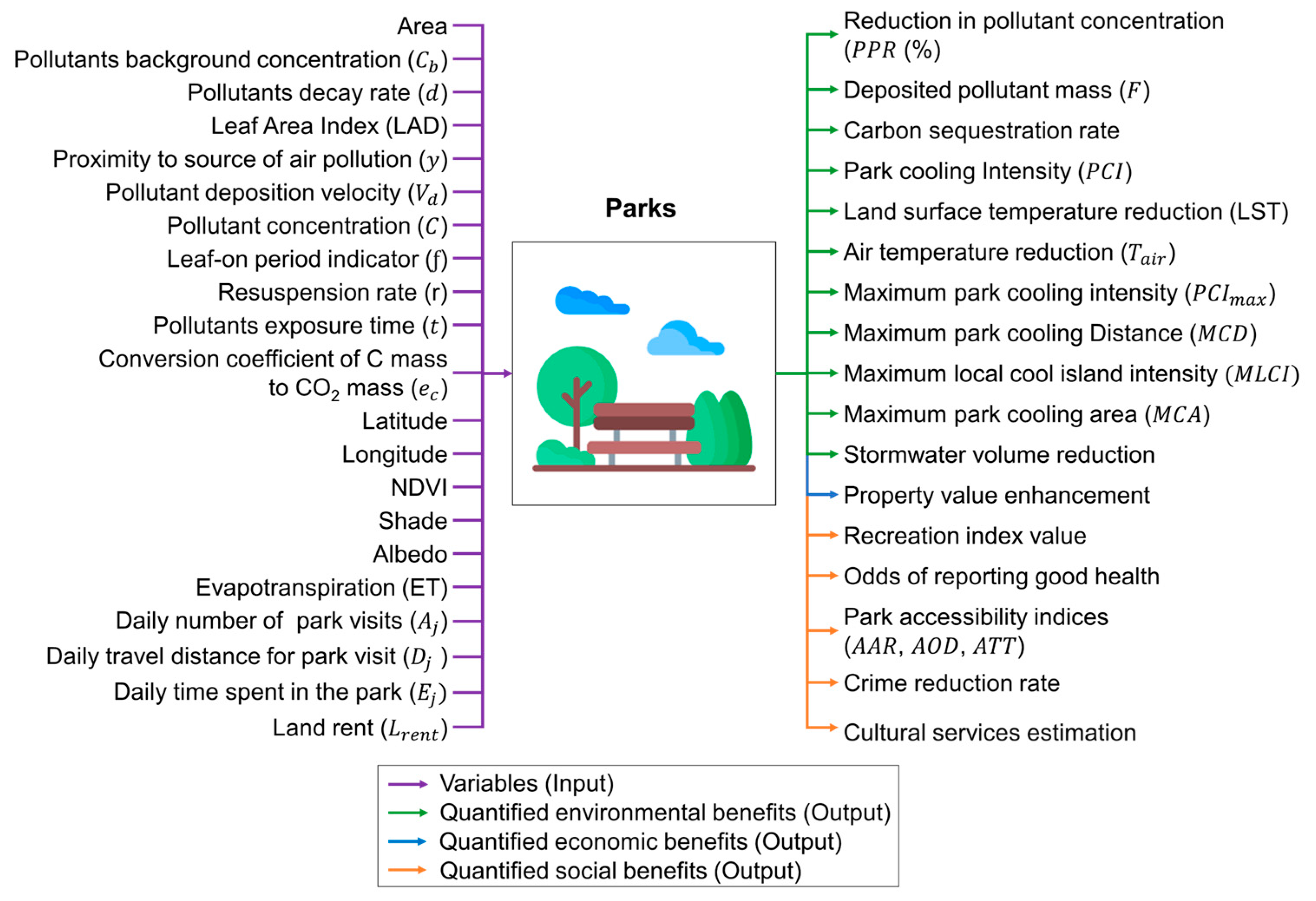
3.6.3. Parks
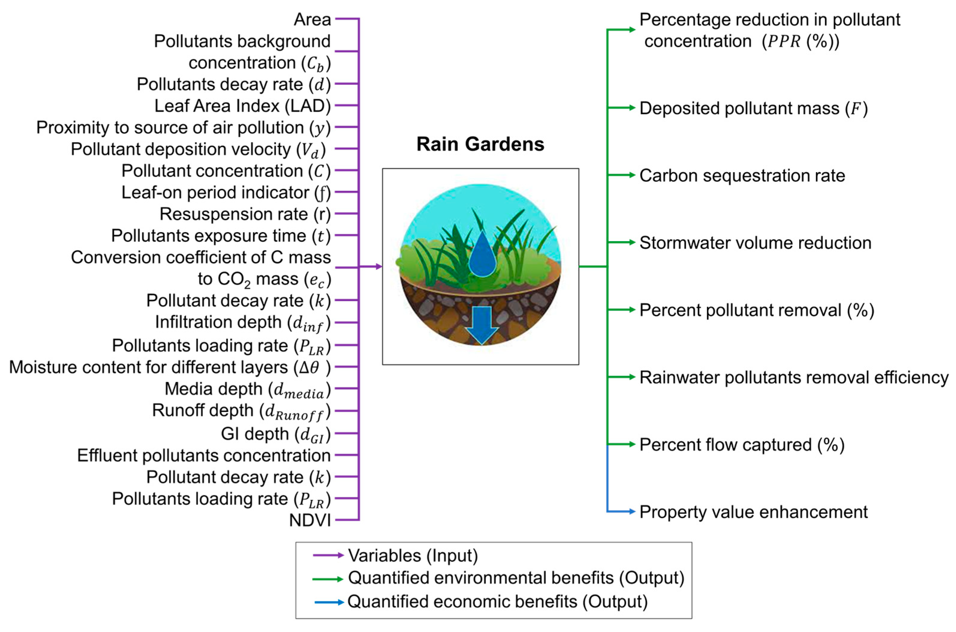
3.6.4. Rain Gardens
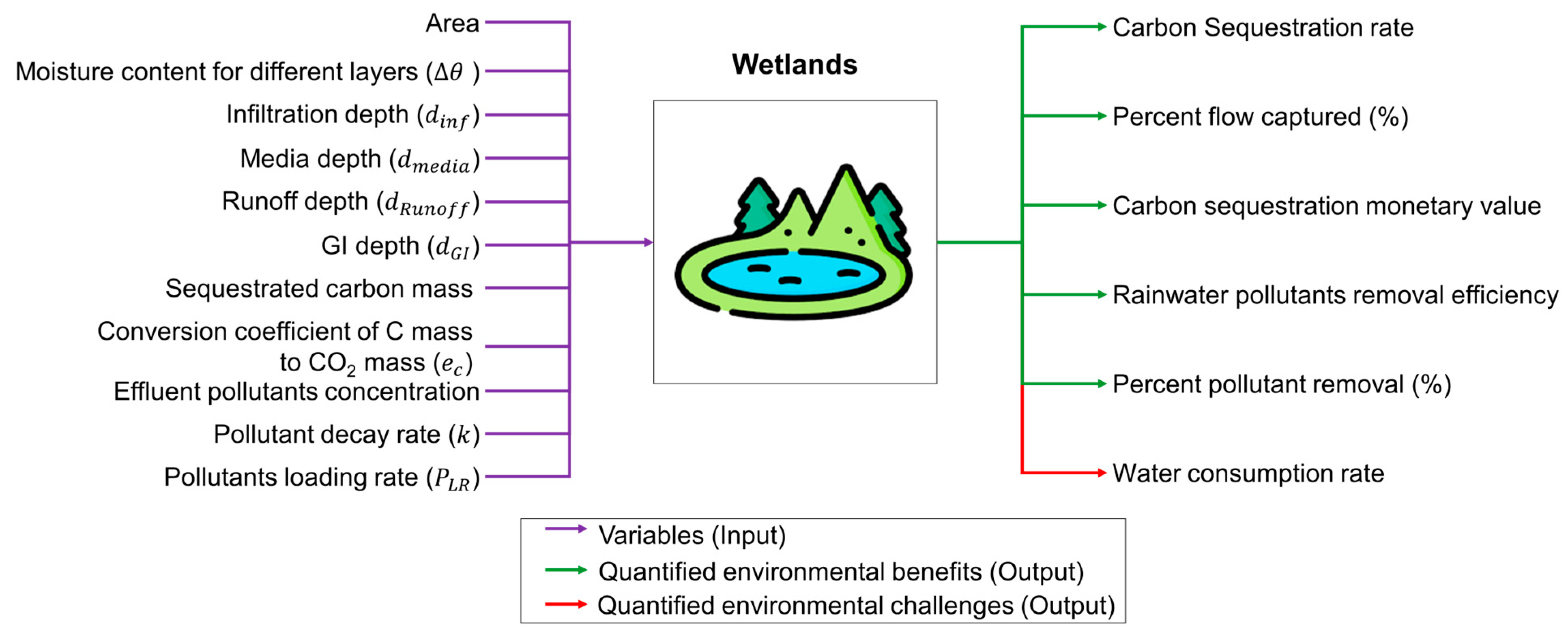
3.6.5. Wetlands
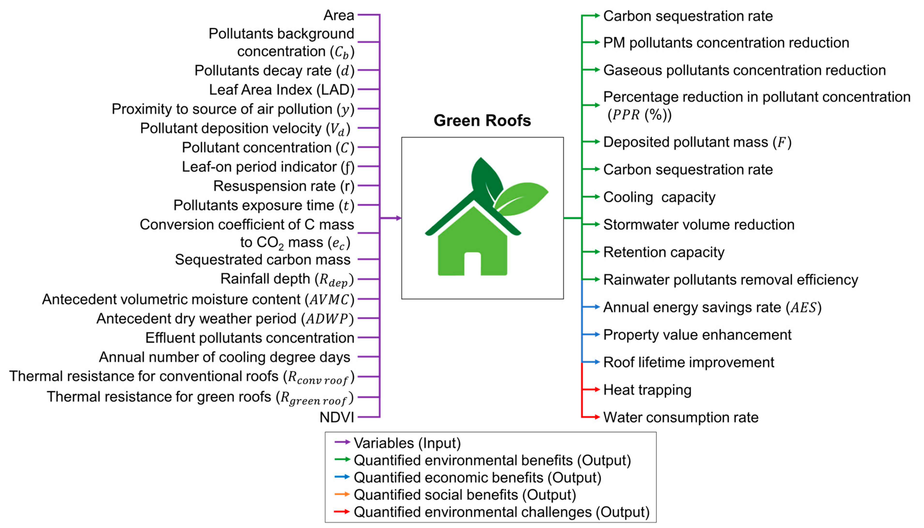
3.6.6. Green Roofs
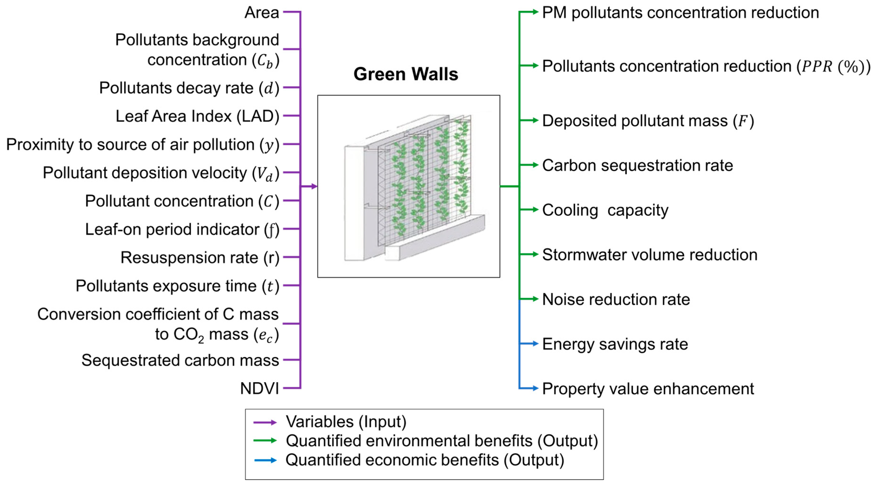
3.6.7. Green Walls
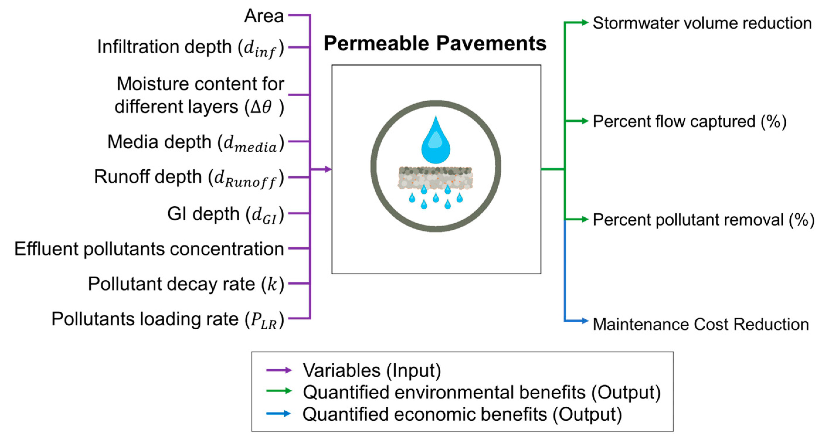
3.6.8. Permeable Pavements
4. Discussion
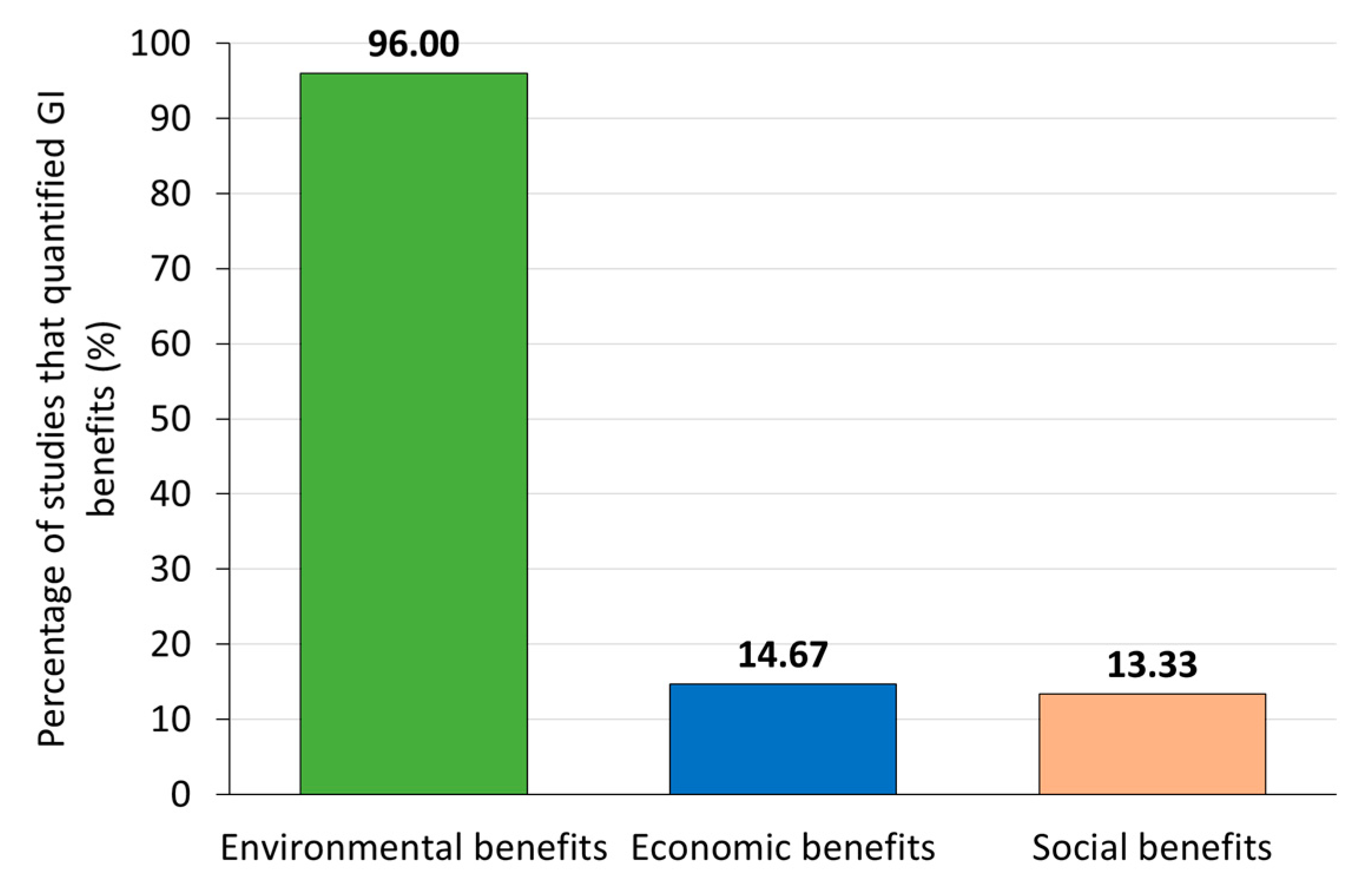
4.1. Quantified Benefits of GIs
4.2. Quantified Challenges of GIs
4.3. GI Types
5. Contributions and Implications
6. Conclusions and Future Work
Author Contributions
Funding
Institutional Review Board Statement
Informed Consent Statement
Data Availability Statement
Conflicts of Interest
References
- United Nations, Department of Economic and Social Affairs. World Urbanization Prospects The 2018 Revision; United Nations: New York, NY, USA, 2018. [Google Scholar]
- Center for Sustainable Systems, University of Michigan. U.S. Cities Factsheet. In Built Environment; Pub. No. C.-06; Center for Sustainable Systems, University of Michigan: Ann Arbor, MI, USA, 2022. [Google Scholar]
- Awumbila, M. Drivers of Migration and Urbanization in Africa: Key Trends and Issues. In Proceedings of the UN Expert Group Meeting on Sustainable Cities, Human Mobility and International Migration, New York, NY, USA, 7–8 September 2017. [Google Scholar]
- Buckley, R.M.; Annez, P.C.; Spence, M. Urbanization and Growth; World Bank Publications: Washington, DC, USA, 2008. [Google Scholar]
- Parr, T.B.; Smucker, N.J.; Bentsen, C.N.; Neale, M.W. Potential Roles of Past, Present, and Future Urbanization Characteristics in Producing Varied Stream Responses. In Freshwater Science; University of Chicago Press: Chicago, IL, USA, 2016; pp. 436–443. [Google Scholar] [CrossRef]
- Dhakal, K.P.; Chevalier, L.R. Managing Urban Stormwater for Urban Sustainability: Barriers and Policy Solutions for Green Infrastructure Application. J. Environ. Manag. 2017, 203, 171–181. [Google Scholar] [CrossRef]
- Xie, L.; Shu, X.; Kotze, D.J.; Kuoppamäki, K.; Timonen, S.; Lehvävirta, S. Plant Growth-Promoting Microbes Improve Stormwater Retention of a Newly-Built Vertical Greenery System. J. Environ. Manag. 2022, 323. [Google Scholar] [CrossRef]
- Sarni, W. The Case for Green Infrastructure in LAC Conclusions from Stockholm World Water Week 2018; 2019. Available online: http://www.iadb.org (accessed on 20 December 2022).
- Tzoulas, K.; Korpela, K.; Venn, S.; Yli-Pelkonen, V.; Kaźmierczak, A.; Niemela, J.; James, P. Promoting Ecosystem and Human Health in Urban Areas Using Green Infrastructure: A Literature Review. In Landscape and Urban Planning; Elsevier: Amsterdam, The Netherlands, 2007; pp. 167–178. [Google Scholar] [CrossRef]
- Venkataramanan, V.; Lopez, D.; McCuskey, D.J.; Kiefus, D.; McDonald, R.I.; Miller, W.M.; Packman, A.I.; Young, S.L. Knowledge, Attitudes, Intentions, and Behavior Related to Green Infrastructure for Flood Management: A Systematic Literature Review. Sci. Total Environ. 2020, 720, 137606. [Google Scholar] [CrossRef] [PubMed]
- Norton, B.A.; Coutts, A.M.; Livesley, S.J.; Harris, R.J.; Hunter, A.M.; Williams, N.S.G. Planning for Cooler Cities: A Framework to Prioritise Green Infrastructure to Mitigate High Temperatures in Urban Landscapes. Landsc. Urban Plan 2015, 134, 127–138. [Google Scholar] [CrossRef]
- Filazzola, A.; Shrestha, N.; MacIvor, J.S. The Contribution of Constructed Green Infrastructure to Urban Biodiversity: A Synthesis and Meta-analysis. J. Appl. Ecol. 2019, 56, 2131–2143. [Google Scholar] [CrossRef]
- Demuzere, M.; Orru, K.; Heidrich, O.; Olazabal, E.; Geneletti, D.; Orru, H.; Bhave, A.G.; Mittal, N.; Feliú, E.; Faehnle, M. Mitigating and adapting to climate change: Multi-functional and multi-scale assessment of green urban infrastructure. J. Environ. Manag. 2014, 146, 107–115. [Google Scholar] [CrossRef] [PubMed]
- Byrne, J.A.; Lo, A.Y.; Jianjun, Y. Residents’ Understanding of the Role of Green Infrastructure for Climate Change Adaptation in Hangzhou, China. Landsc. Urban Plan 2015, 138, 132–143. [Google Scholar] [CrossRef]
- Choi, C.; Berry, P.; Smith, A. The Climate Benefits, Co-Benefits, and Trade-Offs of Green Infrastructure: A Systematic Literature Review. J. Environ. Manag. 2021, 291, 112583. [Google Scholar] [CrossRef] [PubMed]
- Wang, Y.; Ni, Z.; Hu, M.; Li, J.; Wang, Y.; Lu, Z.; Chen, S.; Xia, B. Environmental Performances and Energy Efficiencies of Various Urban Green Infrastructures: A Life-Cycle Assessment. J. Clean Prod. 2020, 248. [Google Scholar] [CrossRef]
- Jim, C.Y. Assessing Climate-Adaptation Effect of Extensive Tropical Green Roofs in Cities. Landsc. Urban Plan 2015, 138, 54–70. [Google Scholar] [CrossRef]
- Huang, B.; Yao, Z.; Pearce, J.R.; Feng, Z.; Browne, A.J.; Pan, Z.; Liu, Y. Non-linear association between residential greenness and general health among old adults in China. Landsc. Urban Plan. 2022, 223, 104406. [Google Scholar] [CrossRef]
- Venter, Z.S.; Shackleton, C.; Faull, A.; Lancaster, L.; Breetzke, G.; Edelstein, I. Is Green Space Associated with Reduced Crime? A National-Scale Study from the Global South. Sci. Total Environ. 2022, 825. [Google Scholar] [CrossRef]
- Liu, Y.; Wang, R.; Grekousis, G.; Liu, Y.; Yuan, Y.; Li, Z. Neighbourhood Greenness and Mental Wellbeing in Guangzhou, China: What Are the Pathways? Landsc. Urban Plan 2019, 190. [Google Scholar] [CrossRef]
- Walker, R.H. Engineering Gentrification: Urban Redevelopment, Sustainability Policy, and Green Stormwater Infrastructure in Minneapolis. J. Environ. Policy Plan. 2021, 23, 646–664. [Google Scholar] [CrossRef]
- Moher, D.; Liberati, A.; Tetzlaff, J.; Altman, D.G.; Liberati, A.; Altman, D.G. Reprint-Preferred Reporting Items for Systematic Reviews and Meta-Analyses: The PRISMA Statement; 2009. Available online: http://www.annals.org/cgi/content/full/151/4/264 (accessed on 27 April 2023).
- Berardi, U.; GhaffarianHoseini, A.; GhaffarianHoseini, A. State-of-the-Art Analysis of the Environmental Benefits of Green Roofs. Appl. Energy 2014, 115, 411–428. [Google Scholar] [CrossRef]
- Tomson, M.; Kumar, P.; Barwise, Y.; Perez, P.; Forehead, H.; French, K.; Morawska, L.; Watts, J.F. Green Infrastructure for Air Quality Improvement in Street Canyons. In Environment International; Elsevier Ltd.: Amsterdam, The Netherlands, 2021. [Google Scholar] [CrossRef]
- Liu, O.Y.; Russo, A. Assessing the contribution of urban green spaces in green infrastructure strategy planning for urban ecosystem conditions and services. Sustain. Cities Soc. 2021, 68, 102772. [Google Scholar] [CrossRef]
- Chen, H.S.; Lin, Y.C.; Chiueh, P.T. High-resolution spatial analysis for the air quality regulation service from urban vegetation: A case study of Taipei City. Sustain. Cities Soc. 2022, 83, 103976. [Google Scholar] [CrossRef]
- Weerakkody, U.; Dover, J.W.; Mitchell, P.; Reiling, K. Quantification of the Traffic-Generated Particulate Matter Capture by Plant Species in a Living Wall and Evaluation of the Important Leaf Characteristics. Sci. Total Environ. 2018, 635, 1012–1024. [Google Scholar] [CrossRef]
- Alves, A.; Gersonius, B.; Kapelan, Z.; Vojinovic, Z.; Sanchez, A. Assessing the Co-Benefits of Green-Blue-Grey Infrastructure for Sustainable Urban Flood Risk Management. J. Environ. Manag. 2019, 239, 244–254. [Google Scholar] [CrossRef]
- Barwise, Y.; Kumar, P.; Tiwari, A.; Rafi-Butt, F.; McNabola, A.; Cole, S.; Field, B.C.T.; Fuller, J.; Mendis, J.; Wyles, K.J. The Co-Development of HedgeDATE, a Public Engagement and Decision Support Tool for Air Pollution Exposure Mitigation by Green Infrastructure. Sustain. Cities Soc. 2021, 75. [Google Scholar] [CrossRef]
- Tiwari, A.; Kumar, P. Integrated Dispersion-Deposition Modelling for Air Pollutant Reduction via Green Infrastructure at an Urban Scale. Sci. Total Environ. 2020, 723, 138078. [Google Scholar] [CrossRef] [PubMed]
- Tiwari, A.; Kumar, P. Quantification of Green Infrastructure Effects on Airborne Nanoparticles Dispersion at an Urban Scale. Sci. Total Environ. 2022, 838, 155778. [Google Scholar] [CrossRef] [PubMed]
- Ramyar, R.; Saeedi, S.; Bryant, M.; Davatgar, A.; Mortaz Hedjri, G. Ecosystem Services Mapping for Green Infrastructure Planning–The Case of Tehran. Sci. Total Environ. 2020, 703, 135466. [Google Scholar] [CrossRef]
- Schmidt, J.P.; Moore, R.; Alber, M. Integrating Ecosystem Services and Local Government Finances into Land Use Planning: A Case Study from Coastal Georgia. Landsc. Urban Plan 2014, 122, 56–67. [Google Scholar] [CrossRef]
- Chen, Y.; Ge, Y.; Yang, G.; Wu, Z.; Du, Y.; Mao, F.; Liu, S.; Xu, R.; Qu, Z.; Xu, B.; et al. Inequalities of Urban Green Space Area and Ecosystem Services along Urban Center-Edge Gradients. Landsc. Urban Plan 2022, 217. [Google Scholar] [CrossRef]
- Doick, K.J.; Peace, A.; Hutchings, T.R. The Role of One Large Greenspace in Mitigating London’s Nocturnal Urban Heat Island. Sci. Total Environ. 2014, 493, 662–671. [Google Scholar] [CrossRef]
- Du, C.; Jia, W.; Chen, M.; Yan, L.; Wang, K. How Can Urban Parks Be Planned to Maximize Cooling Effect in Hot Extremes? Linking Maximum and Accumulative Perspectives. J. Environ. Manag. 2022, 317. [Google Scholar] [CrossRef]
- Shi, D.; Song, J.; Huang, J.; Zhuang, C.; Guo, R.; Gao, Y. Synergistic Cooling Effects (SCEs) of Urban Green-Blue Spaces on Local Thermal Environment: A Case Study in Chongqing, China. Sustain. Cities Soc. 2020, 55. [Google Scholar] [CrossRef]
- Razzaghmanesh, M.; Borst, M.; Liu, J.; Ahmed, F.; O’Connor, T.; Selvakumar, A. Air Temperature Reductions at the Base of Tree Canopies. J Sustain. Water Built. Environ. 2021, 7, 04021010. [Google Scholar] [CrossRef]
- Alim, M.A.; Rahman, A.; Tao, Z.; Garner, B.; Griffith, R.; Liebman, M. Green Roof as an Effective Tool for Sustainable Urban Development: An Australian Perspective in Relation to Stormwater and Building Energy Management. J. Clean. Prod. 2022, 362, 132561. [Google Scholar] [CrossRef]
- Marando, F.; Heris, M.P.; Zulian, G.; Udías, A.; Mentaschi, L.; Chrysoulakis, N.; Parastatidis, D.; Maes, J. Urban Heat Island Mitigation by Green Infrastructure in European Functional Urban Areas. Sustain. Cities Soc. 2022, 77, 103564. [Google Scholar] [CrossRef]
- Zhuang, Q.; Lu, Z. Optimization of Roof Greening Spatial Planning to Cool Down the Summer of the City. Sustain. Cities Soc. 2021, 74, 103221. [Google Scholar] [CrossRef]
- Dong, J.; Peng, J.; He, X.; Corcoran, J.; Qiu, S.; Wang, X. Heatwave-Induced Human Health Risk Assessment in Megacities Based on Heat Stress-Social Vulnerability-Human Exposure Framework. Landsc. Urban Plan 2020, 203, 103907. [Google Scholar] [CrossRef]
- Rocha, A.D.; Vulova, S.; Meier, F.; Förster, M.; Kleinschmit, B. Mapping Evapotranspirative and Radiative Cooling Services in an Urban Environment. Sustain. Cities Soc. 2022, 85, 104051. [Google Scholar] [CrossRef]
- Feyisa, G.L.; Dons, K.; Meilby, H. Efficiency of Parks in Mitigating Urban Heat Island Effect: An Example from Addis Ababa. Landsc. Urban Plan 2014, 123, 87–95. [Google Scholar] [CrossRef]
- Cheng, X.; Wei, B.; Chen, G.; Li, J.; Song, C. Influence of Park Size and Its Surrounding Urban Landscape Patterns on the Park Cooling Effect. J Urban Plan Dev. 2015, 141, A4014002. [Google Scholar] [CrossRef]
- Venter, Z.S.; Krog, N.H.; Barton, D.N. Linking Green Infrastructure to Urban Heat and Human Health Risk Mitigation in Oslo, Norway. Sci. Total Environ. 2020, 709, 136193. [Google Scholar] [CrossRef]
- Liu, Y.; Engel, B.A.; Flanagan, D.C.; Gitau, M.W.; McMillan, S.K.; Chaubey, I. A Review on Effectiveness of Best Management Practices in Improving Hydrology and Water Quality: Needs and Opportunities. Sci. Total Environ. 2017, 601, 580–593. [Google Scholar] [CrossRef]
- Li, S.; Kazemi, H.; Rockaway, T.D. Performance Assessment of Stormwater GI Practices Using Artificial Neural Networks. Sci. Total Environ. 2019, 651, 2811–2819. [Google Scholar] [CrossRef]
- Mason, E.; Montalto, F.A. The Overlooked Role of New York City Urban Yards in Mitigating and Adapting to Climate Change. Local Environ. 2015, 20, 1412–1427. [Google Scholar] [CrossRef]
- Ebrahimian, A.; Wadzuk, B.; Traver, R. Evapotranspiration in Green Stormwater Infrastructure Systems. Sci. Total Environ. 2019, 688, 797–810. [Google Scholar] [CrossRef]
- Shojaeizadeh, A.; Geza, M.; Hogue, T.S. GIP-SWMM: A New Green Infrastructure Placement Tool Coupled with SWMM. J. Environ. Manag. 2021, 277, 111409. [Google Scholar] [CrossRef] [PubMed]
- Dai, X.; Wang, L.; Tao, M.; Huang, C.; Sun, J.; Wang, S. Assessing the Ecological Balance between Supply and Demand of Blue-Green Infrastructure. J. Environ. Manag. 2021, 288, 112454. [Google Scholar] [CrossRef] [PubMed]
- van Oorschot, J.; Sprecher, B.; van ’t Zelfde, M.; van Bodegom, P.M.; van Oudenhoven, A.P.E. Assessing Urban Ecosystem Services in Support of Spatial Planning in the Hague, the Netherlands. Landsc. Urban Plan 2021, 214, 104195. [Google Scholar] [CrossRef]
- Li, C.; Liu, M.; Hu, Y.; Zhou, R.; Wu, W.; Huang, N. Evaluating the Runoff Storage Supply-Demand Structure of Green Infrastructure for Urban Flood Management. J. Clean Prod. 2021, 280, 124420. [Google Scholar] [CrossRef]
- Wong, G.K.L.; Jim, C.Y. Identifying Keystone Meteorological Factors of Green-Roof Stormwater Retention to Inform Design and Planning. Landsc. Urban Plan 2015, 143, 173–182. [Google Scholar] [CrossRef]
- Fan, G.; Lin, R.; Wei, Z.; Xiao, Y.; Shangguan, H.; Song, Y. Effects of Low Impact Development on the Stormwater Runoff and Pollution Control. Sci. Total Environ. 2022, 805, 150404. [Google Scholar] [CrossRef]
- Gong, Y.; Zhang, X.; Li, H.; Zhang, X.; He, S.; Miao, Y. A Comparison of the Growth Status, Rainfall Retention and Purification Effects of Four Green Roof Plant Species. J. Environ. Manag. 2021, 278, 111451. [Google Scholar] [CrossRef]
- Fu, X.; Hopton, M.E.; Wang, X.; Goddard, H.; Liu, H. A Runoff Trading System to Meet Watershed-Level Stormwater Reduction Goals with Parcel-Level Green Infrastructure Installation. Sci. Total Environ. 2019, 689, 1149–1159. [Google Scholar] [CrossRef]
- Martin-Mikle, C.J.; de Beurs, K.M.; Julian, J.P.; Mayer, P.M. Identifying Priority Sites for Low Impact Development (LID) in a Mixed-Use Watershed. Landsc. Urban Plan 2015, 140, 29–41. [Google Scholar] [CrossRef]
- Gavrić, S.; Leonhardt, G.; Marsalek, J.; Viklander, M. Processes Improving Urban Stormwater Quality in Grass Swales and Filter Strips: A Review of Research Findings. Sci. Total Environ. 2019, 669, 431–447. [Google Scholar] [CrossRef]
- Hoyle, H.; Hitchmough, J.; Jorgensen, A. All about the ‘Wow Factor’? The Relationships between Aesthetics, Restorative Effect and Perceived Biodiversity in Designed Urban Planting. Landsc. Urban Plan 2017, 164, 109–123. [Google Scholar] [CrossRef]
- Matos, P.; Vieira, J.; Rocha, B.; Branquinho, C.; Pinho, P. Modeling the Provision of Air-Quality Regulation Ecosystem Service Provided by Urban Green Spaces Using Lichens as Ecological Indicators. Sci. Total Environ. 2019, 665, 521–530. [Google Scholar] [CrossRef]
- Wong, G.K.L.; Jim, C.Y. Do Vegetated Rooftops Attract More Mosquitoes? Monitoring Disease Vector Abundance on Urban Green Roofs. Sci. Total Environ. 2016, 573, 222–232. [Google Scholar] [CrossRef] [PubMed]
- Mitsova, D.; Shuster, W.; Wang, X. A Cellular Automata Model of Land Cover Change to Integrate Urban Growth with Open Space Conservation. Landsc. Urban Plan 2011, 99, 141–153. [Google Scholar] [CrossRef]
- Wang, J.; Rienow, A.; David, M.; Albert, C. Green Infrastructure Connectivity Analysis across Spatiotemporal Scales: A Transferable Approach in the Ruhr Metropolitan Area, Germany. Sci. Total Environ. 2022, 813, 152463. [Google Scholar] [CrossRef]
- Chen, D.; Zhang, F.; Zhang, M.; Meng, Q.; Jim, C.Y.; Shi, J.; Tan, M.L.; Ma, X. Landscape and Vegetation Traits of Urban Green Space Can Predict Local Surface Temperature. Sci. Total Environ. 2022, 825, 154006. [Google Scholar] [CrossRef] [PubMed]
- Deutscher, J.; Kupec, P.; Kučera, A.; Urban, J.; Ledesma, J.L.J.; Futter, M. Ecohydrological Consequences of Tree Removal in an Urban Park Evaluated Using Open Data, Free Software and a Minimalist Measuring Campaign. Sci. Total Environ. 2019, 655, 1495–1504. [Google Scholar] [CrossRef]
- Scheidl, C.; Heiser, M.; Kamper, S.; Thaler, T.; Klebinder, K.; Nagl, F.; Lechner, V.; Markart, G.; Rammer, W.; Seidl, R. The Influence of Climate Change and Canopy Disturbances on Landslide Susceptibility in Headwater Catchments. Sci. Total Environ. 2020, 742, 140588. [Google Scholar] [CrossRef]
- Koroxenidis, E.; Theodosiou, T. Comparative Environmental and Economic Evaluation of Green Roofs under Mediterranean Climate Conditions – Extensive Green Roofs a Potentially Preferable Solution. J. Clean. Prod. 2021, 311, 127563. [Google Scholar] [CrossRef]
- Shih, W.Y. Socio-Ecological Inequality in Heat: The Role of Green Infrastructure in a Subtropical City Context. Landsc. Urban Plan 2022, 226, 104506. [Google Scholar] [CrossRef]
- Neumann, V.A.; Hack, J. Revealing and Assessing the Costs and Benefits of Nature-Based Solutions within a Real-World Laboratory in Costa Rica. Environ. Impact Assess Rev. 2022, 93, 106737. [Google Scholar] [CrossRef]
- Tiwary, A.; Kumar, P. Impact Evaluation of Green-Grey Infrastructure Interaction on Built-Space Integrity: An Emerging Perspective to Urban Ecosystem Service. Sci. Total Environ. 2014, 487, 350–360. [Google Scholar] [CrossRef] [PubMed]
- Maas, J.; Verheij, R.A.; Groenewegen, P.P.; de Vries, S.; Spreeuwenberg, P. Green Space, Urbanity, and Health: How Strong Is the Relation? J. Epidemiol. Community Health 2006, 60, 587–592. [Google Scholar] [CrossRef] [PubMed]
- Derkzen, M.L.; van Teeffelen, A.J.A.; Verburg, P.H. REVIEW: Quantifying Urban Ecosystem Services Based on High-Resolution Data of Urban Green Space: An Assessment for Rotterdam, the Netherlands. J. Appl. Ecol. 2015, 52, 1020–1032. [Google Scholar] [CrossRef]
- Xiao, Y.; Wang, D.; Fang, J. Exploring the Disparities in Park Access through Mobile Phone Data: Evidence from Shanghai, China. Landsc. Urban Plan 2019, 181, 80–91. [Google Scholar] [CrossRef]
- Navarrete-Hernandez, P.; Laffan, K. A Greener Urban Environment: Designing Green Infrastructure Interventions to Promote Citizens’ Subjective Wellbeing. Landsc. Urban Plan 2019, 191, 103618. [Google Scholar] [CrossRef]
- Song, S.; Lim, M.S.; Richards, D.R.; Tan, H.T.W. Utilization of the Food Provisioning Service of Urban Community Gardens: Current Status, Contributors and Their Social Acceptance in Singapore. Sustain. Cities Soc. 2022, 76, 103368. [Google Scholar] [CrossRef]
- Langemeyer, J.; Camps-Calvet, M.; Calvet-Mir, L.; Barthel, S.; Gómez-Baggethun, E. Stewardship of Urban Ecosystem Services: Understanding the Value(s) of Urban Gardens in Barcelona. Landsc. Urban Plan 2018, 170, 79–89. [Google Scholar] [CrossRef]
- Hurley, P.T.; Emery, M.R. Locating Provisioning Ecosystem Services in Urban Forests: Forageable Woody Species in New York City, USA. Landsc. Urban Plan 2018, 170, 266–275. [Google Scholar] [CrossRef]
- Fitzky, A.C.; Sandén, H.; Karl, T.; Fares, S.; Calfapietra, C.; Grote, R.; Saunier, A.; Rewald, B. The Interplay Between Ozone and Urban Vegetation—BVOC Emissions, Ozone Deposition, and Tree Ecophysiology. Front. For. Glob. Chang. 2019, 2, 50. [Google Scholar] [CrossRef]
- Reyes-Paecke, S.; Gironás, J.; Melo, O.; Vicuña, S.; Herrera, J. Irrigation of Green Spaces and Residential Gardens in a Mediterranean Metropolis: Gaps and Opportunities for Climate Change Adaptation. Landsc. Urban Plan 2019, 182, 34–43. [Google Scholar] [CrossRef]
- Houdeshel, C.D.; Hultine, K.R.; Johnson, N.C.; Pomeroy, C.A. Evaluation of Three Vegetation Treatments in Bioretention Gardens in a Semi-Arid Climate. Landsc. Urban Plan 2015, 135, 62–72. [Google Scholar] [CrossRef]
- Razzaghmanesh, M.; Beecham, S.; Brien, C.J. Developing Resilient Green Roofs in a Dry Climate. Sci. Total Environ. 2014, 490, 579–589. [Google Scholar] [CrossRef] [PubMed]
- Rabbani, M.; Kazemi, F. Water Need and Water Use Efficiency of Two Plant Species in Soil-Containing and Soilless Substrates under Green Roof Conditions. J. Environ. Manag. 2022, 302, 113950. [Google Scholar] [CrossRef] [PubMed]
- Wolch, J.R.; Byrne, J.; Newell, J.P. Urban Green Space, Public Health, and Environmental Justice: The Challenge of Making Cities ‘Just Green Enough’. Landsc. Urban Plan 2014, 125, 234–244. [Google Scholar] [CrossRef]
- Pearsall, H. From Brown to Green? Assessing Social Vulnerability to Environmental Gentrification in New York City. Environ. Plan. C Gov. Policy 2010, 28, 872–886. [Google Scholar] [CrossRef]
- Rigolon, A.; Németh, J. Green Gentrification or ‘Just Green Enough’: Do Park Location, Size and Function Affect Whether a Place Gentrifies or Not? Urban Stud. 2020, 57, 402–420. [Google Scholar] [CrossRef]
- Fernández-Alvarado, J.F.; Coloma-Miró, J.F.; Cortés-Pérez, J.P.; García-García, M.; Fernández-Rodríguez, S. Proposing a Sustainable Urban 3D Model to Minimize the Potential Risk Associated with Green Infrastructure by Applying Engineering Tools. Sci. Total Environ. 2022, 812, 152312. [Google Scholar] [CrossRef]
- Rodríguez-Amigo, A.; Fernández-Alvarado, J.F.; Fernández-Rodríguez, S. Case of Study on a Sustainability Building: Environmental Risk Assessment Related with Allergenicity from Air Quality Considering Meteorological and Urban Green Infrastructure Data on BIM. Sci. Total Environ. 2022, 838, 155910. [Google Scholar] [CrossRef]
- Malaviya, P.; Sharma, R.; Sharma, P.K. Rain Gardens as Stormwater Management Tool. In Sustainable Green Technologies for Environmental Management; Springer Singapore: Singapore, 2019; pp. 141–166. [Google Scholar] [CrossRef]
- Scholz, M.; Lee, B. Constructed Wetlands: A Review. Int. J. Environ. Stud. 2005, 62, 421–447. [Google Scholar] [CrossRef]
- Abass, F.; Ismail, L.H.; Wahab, I.A.; Elgadi, A.A. A Review of Green Roof: Definition, History, Evolution and Functions. IOP Conf. Ser. Mater. Sci. Eng. 2020, 713, 012048. [Google Scholar] [CrossRef]
- Manso, M.; Castro-Gomes, J. Green Wall Systems: A Review of Their Characteristics. Renew. Sustain. Energy Rev. 2015, 41, 863–871. [Google Scholar] [CrossRef]
- Imran, H.M.; Akib, S.; Karim, M.R. Permeable Pavement and Stormwater Management Systems: A Review. Environ. Technol. 2013, 34, 2649–2656. [Google Scholar] [CrossRef]
- Carsell, K.M.; Pingel, N.D.; Ford, D.T. Quantifying the Benefit of a Flood Warning System. Nat. Hazards Rev. 2004, 5, 131–140. [Google Scholar] [CrossRef]
- Mihǎilescu, N.; Daescu, V.; Holban, E.; Badea, M.N.; Paceagiu, J. Energy Conservation and CO2 Emissions Reduction for Clinker Portland Cement Manufacturing Process. In Environmental Engineering and Management Journal; Gheorghe Asachi Technical University of Iasi: Iasi, Romania, 2009; Volume 8, pp. 947–952. [Google Scholar] [CrossRef]
- Nieuwenhuijsen, M.J. Green Infrastructure and Health. Annu. Rev. Public Health 2021, 42, 317–328. [Google Scholar] [CrossRef] [PubMed]
- Krauze, K.; Wagner, I. From Classical Water-Ecosystem Theories to Nature-Based Solutions — Contextualizing Nature-Based Solutions for Sustainable City. Sci. Total Environ. 2019, 655, 697–706. [Google Scholar] [CrossRef] [PubMed]
- Easton, S.; Lees, L.; Hubbard, P.; Tate, N. Measuring and Mapping Displacement: The Problem of Quantification in the Battle against Gentrification. Urban Stud. 2020, 57, 286–306. [Google Scholar] [CrossRef]
- Zölch, T.; Rahman, M.A.; Pfleiderer, E.; Wagner, G.; Pauleit, S. Designing Public Squares with Green Infrastructure to Optimize Human Thermal Comfort. Build Environ. 2019, 149, 640–654. [Google Scholar] [CrossRef]
- Matsunaga, S.N.; Shimada, K.; Masuda, T.; Hoshi, J.; Sato, S.; Nagashima, H.; Ueno, H. Emission of Biogenic Volatile Organic Compounds from Trees along Streets and in Urban Parks in Tokyo, Japan. Asian J. Atmos. Environ. 2017, 11, 29–32. [Google Scholar] [CrossRef]


| Quantified Measure | Equation | Definition | Reference | |
|---|---|---|---|---|
| Predicted percentage reduction in pollutant concentration () in % | (1) | is a common measure to quantify the air purification capabilities of GI, where is the pollutant concentration at the area of study without GI (in µ𝗀/m3) and it could be determined using Equation (2); and is the pollutant concentration at the area of study with GI (in µ𝗀/m3) and can be obtained from Equation (3). | [29] | |
| (2) | is the pollutant concentration at the area of study without GI (in µ𝗀/m3), where is the background concentration or the constant concertation that pollution concertation converges to after mixing with air, is the initial concentration of pollutant on the roadway, is its decay rate, and is the defined proximity from the roadway (in m) in which the pollutant concentration is being calculated. | |||
| (3) | is the pollutant concentration at the area of study with GI (in µ𝗀/m3), where is assumed to be the effect of GI on the pollutant concentration reduction as a function of leaf area density (; ), is the distance (in m) from the roadway (source of pollution) to GI, is the distance (in m) from GI to the area of study, and and are GI-induced reduction factors dependent on the pollutant and its interaction with the vegetation barrier. | |||
| Deposited pollutant mass for GI in 𝗀/m2 | (4) | is a measure of the pollutants that are deposited onto vegetation leaves, where is the deposition velocity (in m/s), is the pollutant concentration (in 𝗀/m3), t is the exposure time (in s), f is the leaf-on period indicator and is assumed 0.5 for deciduous trees or 1 for grassland and coniferous trees, and r is the resuspension rate assumed 0.5 for particulate pollutants to account for resuspension of pollutant particles back to the atmosphere. Moreover, depends on the pollutant nature, whether it is a gaseous pollutant (i.e., NO2) or particulate matter (i.e., PM10 and PM2.5), and could be calculated using Equations (5) and (6), respectively. | [30] | |
| (5) | is the deposition velocity (in m/s) for gaseous pollutants, where is the aerodynamic resistance (in s/m), is the quasi-laminar boundary layer resistance (in s/m), and is the surface resistance (in s/m). | |||
| (6) | is the deposition velocity (in m/s) for particulate matter, where is the aerodynamic resistance (in s/m), is the quasi-laminar boundary layer resistance (in s/m), and is the particulate settling velocity (in m/s). | |||
| Total particle number deposition () in #/cm2 | (7) | is another measure of the deposition process, where is expressed in terms of the initial total particle number concentration () in #/cm2, annual deposition time ( = 3.1 × 10⁷ s), the fraction of the in a specific mode such as nucleation (), Aitken (), and accumulation (), and dry deposition velocities in a specific mode such as nucleation () in cm/s, Aitken () in cm/s, and accumulation () in cm/s. | [31] | |
| The removal rate of PM2.5 () in 𝗀/m2 | (8) | is a measure of the urban vegetation deposition rate of PM2.5, where is the deposition velocity of PM2.5 in (m/s), is the concentration of PM2.5 in (µ𝗀/m3), is the vegetation leaf area index in (m2/m2), is the no-rainfall time (in s), is the resuspension rate (in %), is the grid number (where the area of study is divided into grids), and is a notation for the seasons in a year. | [26] | |
| (9) | is the annual total PM2.5 removal (in 𝗀), is the seasonal mean PM2.5 removal rate of vegetation type () (in 𝗀/m2), and is the coverage area of vegetation type () (in m2). | |||
| GI Type | Carbon Storage Value | Unit | Reference |
|---|---|---|---|
| Tree | 0.75, 7.69, 28.46 | k𝗀C/m2 | [13,25,32] |
| Woodland | 28.46 | k𝗀C/m2 | [25] |
| Tall shrub | 14.19 | k𝗀C/m2 | |
| Short shrub | 10.23 | k𝗀C/m2 | |
| Herbaceous | 0.15 | k𝗀C/m2 | |
| Private garden | 0.79 | k𝗀C/m2 | |
| Agricultural land | 0.1 | k𝗀C/m2 | |
| Vegetation | 18, 26, 30.25, 31.4, 31.6, 60, and 141.4 | tC/ha/yr | (Demuzere et al., 2014) [33] |
| Urban land | 4.7, 7.2 | tC/ha/yr | [13,33] |
| Forested wetland | 147 | tC/ha/yr | [33] |
| Tidal brackish wetland | 92 | tC/ha/yr | |
| Freshwater wetland | 95 | tC/ha/yr | |
| Tidal salt wetland | 78 | tC/ha/yr | |
| Green roof | 165 | k𝗀C/m2/yr | [28] |
| Quantified Measure | Equation | Definition | Reference | |
|---|---|---|---|---|
| Cooling index () | (11) | is a valuable measure for determining the optimal amount of urban green vegetation necessary to effectively cool summer temperatures, is the tree cover density (in %), is the average summer land surface temperature (in °C), is a dimensionless empirically-derived constant equals to 5, and 100 is a correction factor. | [40] | |
| Cooling capacity index () (based on raster analysis) | (12) | Another method for quantifying the cooling capacity index () is through the analysis of raster pixels as indicated by Equation (12). The variable is the fraction of light that is reflected by a surface, the variable is extracted from a tree canopy map, and the variable is the evapotranspiration index of each raster pixel. | [41] | |
| Cooling capacity index for large green areas () (larger than 2 ha) | (13) | is considered as a distance weighted average of the cooling capacities of the surrounding green area pixels within a cooling distance (), where equals 1 if pixel j is green, is distance from pixel to pixel . | ||
| Heat mitigation index () | (14) | is a metric used to evaluate the effectiveness of GI in mitigating urban heat islands. is the cooling capacity index calculated based on Equation (12), is the cooling capacity for large green areas calculated based on Equation (13), and is the green area around pixel . | ||
| Microclimate regulation measure () in kWh/m2 of green space/yr (due to tree canopy cover cooling effect) | (15) | The presence of tree canopy cover also contributes to the overall microclimate regulation, where the tree canopy cover cools the urban area by providing shade and increasing evapotranspiration. As shown in Equation (15), is the trees’ biomass (in ton/m2), is the percentage of leaf biomass in tree biomass (8.73%), is the evapotranspiration intensity (451.9 ton of water/ton of fresh leaves/year), is the mean annual precipitation in ton/m2, is the soil evaporation coefficient (5%), is the heat consumed by vaporization of a ton of water (2.26 × 10⁶ kJ), and (in kWh/ kJ) is the conversion factor from kJ to kWh (1/3600). | [34] | |
| Universal thermal climate index () | (16) | is a measure used to represent human thermal comfort perception; where higher values of correspond to higher levels of thermal discomfort. is calculated using Equations (16)–(18) for the main urban area, metropolitan development area, and beyond metropolitan area, respectively; where is the percentage of greenspace area (in %), is the percentage of the water body area (in %), and is the percentage of constructed land area (in %). | [42] | |
| (17) | ||||
| (18) | ||||
| Greening cooling services index () | (19) | is a measure of the cooling services provided by GIs, where it is the average of the evapotranspiration cooling service () and the radiative cooling service () sub-indices as shown in Equations (20) and (21), respectively. Moreover, low index values are an indication of poor evapotranspiration and radiative cooling services, which implies that there is a higher risk of heat exposure. | [43] | |
| (20) | is a measure of the cooling capacity of GIs based on the amount of water released into the atmosphere through evapotranspiration () in mm/day on the hottest day of the year, where and are the maximum and minimum , respectively. | |||
| (21) | is a measure of a plant’s ability to lower the surface temperature through shading and it is calculated based on the maximum hourly soil temperature () in °C, on the hottest day of the year, and the vegetation percentage () in %. Moreover, and are the maximum and minimum , respectively. | |||
| Quantified Measure | Equation | Definition | Reference | |
|---|---|---|---|---|
| Maximum park cooling intensity () in °C | (22) | is a commonly used index to estimate the maximum temperature difference between a park and its surrounding environment, where is a parameter expressing the temperature difference between the park and its wider surrounding, is a NDVI-related coefficient, and the is the normalized difference vegetation index within each ring buffer assumed around the park. | [44] | |
| Park cooling distance () in m | (23) | is a measure of the maximum distance (in m) within which the cooling effect of a park could still be detected, where is the area of the park (in ha), is the park’s shape index (dimensionless), is the park’s mean altitude (in m), and is the park’s longitude (UTM easting in km). Furthermore, , , , , , and are parameters to be estimated. | [44] | |
| Park cooling intensity () in °C | (24) | is the park cooling intensity taking into consideration the proximity to multiple buffers around the park’s edge, where the ring buffer zones are represented by the subscript , is the distance between the park and the ring buffer (in m), is the residual error, and a and b are coefficients calculated using Equations (25) and (26). Moreover, is a coefficient to be estimated. | [44] | |
| (25) | ||||
| (26) | ||||
| Maximum park cooling distance () in m | (27) | is the maximum distance (in m) at which the park can provide cooling, where is the park’s area (in ha). | [45] | |
| Local cool island intensity () in K | (28) | is the maximum intensity of the cooling effect within the immediate area surrounding the park, where is the park’s area (in ha). | [45] | |
| Maximum park cooling area () in ha | (29) | MCA is the maximum area (in ha) over which the park’s cooling effect is felt, where is the park’s area (in ha). | [45] | |
| Land surface temperature () | (30) | Parks’ ability to provide cooling could also be quantified using (in K), where is the park’s area (in ha). | [45] | |
| Quantified Measure | Equation | Definition | Reference | |
|---|---|---|---|---|
| Land surface temperature () in °C (in the presence of tree canopy cover) | (31) | The cooling effect of trees is demonstrated by the negative association of the (°C) and the percentage of tree canopy cover () in %. | [46] | |
| Land surface temperature () in °C (in the presence of vegetation) | (32) | The cooling effect of vegetation is demonstrated by the negative association of the (°C) and the normalized difference vegetation index (see Equation (66)). | [46] | |
| Land surface temperature () in °C (in the presence of tree canopy cover) | (33) | The cooling effect of tree canopy is generally reflected by , where is the tree cover density and is the amount of water evaporated from tree canopies in mm/day. Moreover, , , and are coefficients to be estimated. | [40] | |
| Maximum air temperature () in °C (in the presence of tree canopy cover) | (34) | The cooling effect of tree canopy is also reflected by , where is the latitude of the area of study. Moreover, , , and are coefficients to be estimated. | [40] | |
| Percentage reduction of urban heat island (in %) | (35) | Percentage reduction of urban heat island is a measure used to evaluate the effectiveness of GI in mitigating urban heat islands, where is the temperature of the GI, is the temperature of GI in the rural surrounding, and is the temperature of the built area (i.e, structures and roads). | [47] | |
| Quantified Measure | Equation | Definition | Reference | |
|---|---|---|---|---|
| in % (for infiltration-based GIs) | (36) | is the area of the GI (in m2), is the infiltration depth (in m), is the moisture content for the different layers in the GI, is the entire media depth (in m), is the area of the sub-basin in (m2), is the runoff depth (in m), and is the depth of the GI (in m). | [51] | |
| in % (for storage-based GIs) | (37) | |||
| Surface runoff () in mm | (38) | (in mm) is the mean annual precipitation and (in mm) denotes the maximum potential retention of catchment and could be calculated using Equation (39). | [25,52] | |
| (39) | , the curve number, is a dimensionless parameter used in hydrology to estimate the amount of runoff from a drainage basin. is dependent on the land cover and soil type, where higher values indicate a higher potential for runoff. | [25] | ||
| Runoff retention () in L/m2 | (40) | (in mm) is the mean annual precipitation and is a dimensionless runoff coefficient that could be calculated using Equation (41). | [25,52,53] | |
| (41) | (in mm) is the surface runoff (see Equation (38)) and (in mm) is the mean annual precipitation. | |||
| Rainwater storage capacity of GI () in mm | (42) | and are the vegetation and soil proportions of the GI, respectively; is the maximum canopy storage capacity (in mm) and is calculated based on Equation (43); and is the soil rainwater storage capacity (in mm) and could be calculated as shown in Equation (44). | [54] | |
| (43) | is the leaf area index (see Equations (78) and (79)). | |||
| (44) | is the soil depth (in mm), is the bulk density of the soil (in 𝗀/cm3), and is the particle density of the soil (in 𝗀/cm3). | |||
| Rainwater runoff reduction by green spaces () in ton/yr | (45) | is the average annual precipitation (in m/yr), is the area of the green space (in m2), is the runoff coefficient for impervious surfaces, is the runoff coefficient for the green space, and is the water density assumed equal to 1 ton/m3. | [34] | |
| Retention capacity (R) in % (for green roofs) | (46) | is the rainfall depth (in mm), and is the antecedent volumetric moisture content (in m3/m3). | [55] | |
| (47) | is the rainfall depth (in mm), and is the antecedent dry weather period (in h). | |||
| (48) | rainfall depth (in mm), is the antecedent dry weather period (in h), is the mean wind speed (in m/s), and is the solar radiation (in W/m2). | |||
| Runoff control rate () in % | (49) | could be calculated using Equation (49), where is the runoff after installation of the GI (in m3), is the total runoff of the storm event (in m3). | [56] | |
| (50) | could be also estimated using Equation (50), where is the total rainfall (mm), and is the total runoff (in m). | [57] | ||
| Actual runoff abatement () in m2 (for one GI) | (51) | refers to the measurable reduction in stormwater runoff volume. The of one GI type, , placed on parcel is calculated as per Equation (51), where is the runoff abatement capacity of the GI (in m3), is the runoff depth (in m), and is the parcel’s area (in m2). | [58] | |
| Actual runoff abatement () in m2 (for multiple GIs) | (52) | When considering multiple GI types, having GI type implemented, followed by implementing type on parcel , is then calculated based on Equation (52), where is the runoff abatement capacity of the GI (in m3), is the runoff depth (in m), and is the parcel’s area (in m2). | [58] | |
| Quantified Measure | Equation | Definition | Reference | |
|---|---|---|---|---|
| Percent pollutant removal (in %) (for infiltration-based GI) | (53) | The efficiency of pollutant removal depends on the type of GI used, whether it is infiltration-based or storage-based. For infiltration-based GI it could be calculated using Equation (53), where is the decay rate value for the pollutant (in k𝗀/m3/s), is the entire media depth (in m), is the area of the GI (in m2), and is the pollutants loading rate (in k𝗀/s). | [51] | |
| Percent dissolved pollutant removal (in %)(for storage-based GI) | (54) | Percent dissolved pollutant removal (%) is a measure of the efficiency of pollutant removal in a storage-based GI, where is the decay rate value for the pollutant (in k𝗀/m3/s), is the depth of the GI (in m), is the area of the GI (in m2), and is the pollutants loading rate (in k𝗀/s). | [51] | |
| Percent colloid removal (in %) (for storage-based GI) | (55) | Percent colloid removal (%) refers to the percentage of colloidal particles (e.g., small suspended solids or pollutants) that are removed from stormwater runoff by a GI, where is the kinematic viscosity of water (in m2/s), is the average diameter of the grains (in m), is the volumetric sediment concentration, is the gravitational acceleration (in m/s2), is the submerged specific gravity of the grains that could be calculated using Equation (56), and is the runoff flow (in m3/s). | [51] | |
| (56) | is the submerged specific gravity of the grains, where is the water density (in k𝗀/m3) and is the density of the grains (in k𝗀/m3). | |||
| TSS removal () (in grass swales and grass filter strips) | (57) | is a measure of TSS trapping efficiency, where is the average flow velocity, is the flow area hydraulic radius, is the particle settling velocity, is the length of the grass section, is the kinematic viscosity, and is the flow depth. | [60] | |
| TSS removal () (in grass swales and grass filter strips for smaller sediment particles (0–180 µm) and lower concentrations of sediment in the inflow (670–3920 m𝗀/L)) | (58) | When considering smaller sediment particles (0–180 µm) and lower concentrations of sediment in the inflow (670–3920 m𝗀/L), the quantification described in Equation (57) is no longer effective. In such cases, Equation (58) is recommended to be used as it is considered more representative. As shown in Equation (58), is the distance from the inlet edge to the point of study “X” along the grass section. | [60] | |
| pollution retention rate () in % | (59) | is a measure of the GI effectiveness in reducing pollutant load, where is the outfall pollutant load (in k𝗀) after installation of the GI, and is the outfall pollutant load (in k𝗀) before installing GI. | [56] | |
| (60) | could be also calculated using Equation (60), where is the pollutant mass throughout the runoff process (in m𝗀), and is the pollutant mass throughout the outflow (in m𝗀). | [57] | ||
| Quantified Measure | Equation | Definition | Reference | |
|---|---|---|---|---|
| Lichen species richness | (62) | The lichen trees richness is defined as the total number of lichen species in a green space, where is the green space area (in m2), and is the average NDVI (see Equation (66)) for a 100 m buffer around the green space centroid with the green space area included. | [62] | |
| Simpson’s index of diversity () | (63) | is a measure of species diversity in the ecosystem, where it is unitless and ranges between 0 and 1. A higher value for indicates heterogeneity (i.e., higher diversity), while a lower value indicates a lower degree of diversity (homogeneity). As shown in Equation (63), is the species number, is the frequency of specimens of species, and is the specimens’ total number regardless of species. | [63] | |
| Land use mix index () | (64) | could be used as a measure that assesses the distribution of land use and land cover classes across a landscape, where values close to 1 indicate a blend of various similarly sized land cover classes across the landscape, while values close to 0 indicate a dominance of a particular land cover class. As shown in Equation (64), is the proportion of land cover of type , and is the total number of land cover classes. | [64] | |
| Integral index of connectivity () | (65) | is used to prioritize green and blue spaces, such as habitats and ecological corridors, where evaluates the role of each core area in maintaining and improving the connectivity of the GI network. with higher values indicates more connectivity between GI core area. As shown in Equation (65), is the total number of GI elements in the area of study, and are the areas of the GI elements, is the number of shortest path links between and , and is the total area of the landscape (including habitat and non-habitat areas). | [65] | |
| Normalized difference vegetation index () | (66) | could be used to quantify biodiversityby considering the difference between near-infrared () and red light (), as shown in Equation (66). Since vegetation generally reflects and absorbs , a higher value indicates dense green vegetation. | [66] | |
| Quantified Measure | Equation | Definition | Reference | |
|---|---|---|---|---|
| Slope stability safety factor () | (67) | values larger than one indicate a stable soil column at depth and time As shown in Equation (67), is the depth of layer soil layer , is the internal friction angle for the entire soil depth , is the soil column slope angle (in rad), is the soil moisture of layer at time t and could be calculated as per Equation (68), A is the effective normal stress and could be obtained using Equation (69), and B is the resisting force cohesion angle which is calculated using Equation (70). | [68] | |
| (68) | is the soil moisture of layer at time t, where is the water content of the soil in layer at time, and is the saturated water content of layer . | |||
| (69) | A is the effective normal stress, where is the water-specific weight (in kN/m3), is the pressure developed due to the vegetation weight (in kN/m2), is the depth of layer soil layer is the soil moisture of layer at time t, is the saturated soil specific weight (in kN/m3), and is the dry soil specific weight (in kN/m3). | |||
| (70) | B is the resisting force cohesion angle, where and are the soil and root cohesion (in Pa), respectively. Moreover, is the water-specific weight (in kN/m3) and is the soil column slope angle (in rad). |
| Quantified Measure | Equation | Definition | Reference | |
|---|---|---|---|---|
| Average daily green access () | (73) | could be estimated using Equation (73), where is the daily number of visits of person , is the activity duration per day, is the total number of visitors, and is the total activity duration. | [75] | |
| Average daily travel distance from origin to park () | (74) | could be estimated using Equation (74), where is the daily travel distance of person from the origin to the park, is the activity duration per day, is the total number of visitors, and is the total activity duration. | [75] | |
| Average daily time spent in the park () | (75) | could be estimated using Equation (75), where is the daily time spent in the park of person , is the activity duration per day, is the total number of visitors, and is the total activity duration. | [75] | |
Disclaimer/Publisher’s Note: The statements, opinions and data contained in all publications are solely those of the individual author(s) and contributor(s) and not of MDPI and/or the editor(s). MDPI and/or the editor(s) disclaim responsibility for any injury to people or property resulting from any ideas, methods, instructions or products referred to in the content. |
© 2023 by the authors. Licensee MDPI, Basel, Switzerland. This article is an open access article distributed under the terms and conditions of the Creative Commons Attribution (CC BY) license (https://creativecommons.org/licenses/by/4.0/).
Share and Cite
Jezzini, Y.; Assaf, G.; Assaad, R.H. Models and Methods for Quantifying the Environmental, Economic, and Social Benefits and Challenges of Green Infrastructure: A Critical Review. Sustainability 2023, 15, 7544. https://doi.org/10.3390/su15097544
Jezzini Y, Assaf G, Assaad RH. Models and Methods for Quantifying the Environmental, Economic, and Social Benefits and Challenges of Green Infrastructure: A Critical Review. Sustainability. 2023; 15(9):7544. https://doi.org/10.3390/su15097544
Chicago/Turabian StyleJezzini, Yasser, Ghiwa Assaf, and Rayan H. Assaad. 2023. "Models and Methods for Quantifying the Environmental, Economic, and Social Benefits and Challenges of Green Infrastructure: A Critical Review" Sustainability 15, no. 9: 7544. https://doi.org/10.3390/su15097544
APA StyleJezzini, Y., Assaf, G., & Assaad, R. H. (2023). Models and Methods for Quantifying the Environmental, Economic, and Social Benefits and Challenges of Green Infrastructure: A Critical Review. Sustainability, 15(9), 7544. https://doi.org/10.3390/su15097544