Abstract
In this study, the latest release of all available Coupled Model Intercomparison Project Phase 6 (CMIP6) climate models with two future scenarios of Shared Socio-Economic Pathways, SSP2-4.5 and SSP5-8.5, over the period 2015–2100 are utilized in diagnosing climate extremes in Türkiye. Coarse-resolution climate models were downscaled to a 0.1° × 0.1° (~9 km) spatial resolution using the European Centre for Medium-Range Weather Forecasts Reanalysis 5-Land (ERA5-Land) dataset based on three types of quantile mapping: quantile mapping, detrended quantile mapping, and quantile delta mapping. The temporal variations of the 12 extreme precipitation indices (EPIs) and 12 extreme temperature indices (ETIs) from 2015 to 2100 consistently suggest drier conditions, in addition to more frequent and severe precipitation extremes and warming temperature extremes in Türkiye, under the two future scenarios. The SSP5-8.5 scenario indicates more severe water stress than the SSP2-4.5 scenario; the total precipitation decreases up to 20% for Aegean and Mediterranean regions of Türkiye. Precipitation extremes indicate a decrease in the frequency of heavy rains but an increase in very heavy rains and also an increasing amount of the total precipitation from very heavy rain days. Temperature extremes such as the coldest, warmest, and mean daily maximum temperature are expected to increase across all regions of Türkiye, indicating warming conditions by up to 7.5 °C by the end of the century. Additionally, the coldest daily maximums also exhibit higher variability to climate change in the subregions Aegean, Southeastern Anatolia, Marmara, and Mediterranean regions of Türkiye while the mean daily maximum temperature showed greater sensitivity in the Black Sea, Central Anatolia, and Eastern Anatolia regions.
1. Introduction
Several climatic events such as floods, droughts, fires, and heatwaves have been encountered as a result of global warming and climate change [1,2,3,4,5]. There is a scientific consensus that climatic change and global warming exacerbate the duration, intensity, and frequency of extreme events, which adversely impact different socio-economic sectors worldwide [6,7,8,9]. Furthermore, these climate extremes, which are more sensitive to climate change compared with the average climate, are a top global risk [10]. CRED [11] reports that over the past two decades, extreme temperature events have contributed to 13% of disaster-related human mortality worldwide, while floods have affected 1.65 billion people and droughts have affected 1.45 billion people [9].
On a global scale, previous studies revealed that the intensity and frequency of extreme events have increased, and this increase is expected to continue [10,12,13,14]. However, extreme precipitation events are not spatially consistent so exhibit robust spatial variability while temperature extremes generally exhibit consistent behavior, especially for the frequency, with the global-scale changes [15,16,17]. Therefore, different regional scales reveal different change patterns in extreme climate events, and these variations by region lead to impacts that vary spatiotemporally [6,10,18].
Considering the existing trends of the climate, both moderate- and high-emission scenario results reveal that existing trends will likely persist throughout the 21st century [19]. As variations in climate extremes cause significant socioeconomic impacts [3,20], exploring the changes in climate extremes at the global, regional, and local scales is a major subject to be carefully considered [21,22]. The Expert Team on Sector-specific Climate Indices (ET-SCI) was formed by the World Meteorological Organization (WMO)’s Commission for Climatology (CCl) for developing several climate indices that can be used for various sectoral applications such as water resources, agriculture, or energy [23,24,25,26].
As a centralized and global initiative, the Coupled Model Inter Comparison Project (CMIP) was established to better understand climate changes from the past to the future with the participation of relevant organizations around the world. The initiative has developed several climate models to investigate the predictability of the climate system and to make predictions based on the observed climate [27,28]. The latest phase (Phase 6) of the CMIP, known as CMIP6, is expected to introduce significant advancements compared to its predecessor, CMIP5. These enhancements are attributed to the quantification of radiative forcing, including natural and human-induced factors, the integration of aerosol and land-use effects, and other factors [29,30]. The Köppen–Geiger classification was compared using CMIP5 and CMIP6 data by Bayar [31] and the differences between them were investigated; it was revealed that CMIP6 would have more changes in climate classes due to its warmer predictions. Although CMIP6 is a relatively new phase, the application of those newest projections has gained increasing interest [32,33,34]. Regarding the performance of the CMIP6 and CMIP5 over their study regions, these studies produced varied results. For example, Bağcaci et al. [29] indicated that CMIP6 models perform better than CMIP5 models when they evaluated the changes in precipitation and near-surface temperature in Türkiye. The outperforming CMIP6 results necessitate the re-evaluation of the consequences of impact studies with sector-specific climate indices using the most recent climate data for Türkiye. Even with the outperforming CMIP6 models available, it is not an easy process to assess the impact of climate change on local hydrometeorological extremes. This difficulty mainly arises due to the uncertainty in obtaining information from global coarse-resolution models and transforming those into the local scale [35], which is also the subject of this research.
Considering the improvement in the global climate models’ (GCMs) output performance regionally or locally, extensive research on statistical downscaling, bias correction methods, and their applications related to hydrometeorological impact studies have been carried out. In the bias correction and downscaling process of CMIP6 GCM model data, which will also be used in this study, quantile mapping (QM), quantile delta mapping (QDM), and detrended quantile mapping (DQM) methods will be used. These methods are known to perform better in representing extreme precipitation and changes in temperature in the current literature [36,37,38]. The bias correction applications that rely on statistical approaches mainly employ the observed or modeled high-accuracy historical data to obtain a reference distribution and relationship for the model projections. Furthermore, horizontal resolution is a very important aspect in the accurate simulation of the spatial and temporal evolution of the climatological variables. According to Hersbach et al. [39], reanalysis generates seamless and consistent maps of fundamental climate variables and a logical portrayal of fundamental Earth system cycles by skillfully combining observations and models. The newly represented European Centre for Medium-Range Weather Forecasts (ECMWF) Reanalysis ERA5-Land datasets were used as historical references for the bias-correction process for many studies. ERA5-Land’s temporal resolution is hourly, and the horizontal resolution is 9 km [40].
The Mediterranean region in the globe as a climatic hotspot shows a significant decrease in precipitation and a progressive increase in temperature detected through the climate projections [29,41,42,43,44,45]. Tuel and Eltahir [43] noticed a decrease in winter precipitation, which could reach up to 40% locally in the region. Driouech et al. [44] studied the Middle East and North Africa (MENA) region and projected drying in the north-west and moistening in the north-east side of the Mediterranean region. Moreover, expected warming by 0.2 °C to 0.5 °C per decade over land was also found in the study. As one of the most vulnerable countries in the Mediterranean, Türkiye is expected to experience severe warming and drying and needs critical assessment regarding climate change and its extremes [29,46].
Severe warming and drying risks of an increasing magnitude are becoming more likely in Türkiye [29,47,48,49]. Studies also revealed the possibility of warming winters, especially in the mountainous regions of Eastern Anatolia of Türkiye [50,51,52]. Yucel et al. [52] also indicated significant temperature increases (an average of 1.3 °C across the selected stations) from 1970 to 2010 in eastern Anatolia, Türkiye. Moreover, Aziz et al. [53] investigated CORDEX ensemble model results throughout Türkiye considering the nonstationary impacts and argued that minimum and maximum temperature extremes will occur with higher magnitudes with up to 10 °C and 4 °C, respectively, and less recurrence time according to climate projections under a high-emission scenario. Ozturk [49] found that about 7 °C warming is expected for the maximum temperatures over the Mediterranean region with increasing summer extreme temperatures being likely. Furthermore, Todaro et al. [45] showed that the Konya area in Turkey has warmed up with an annual temperature increase of 0.5 °C/decade in the period 1976–2005 and will face a significant drought effect based on the increasing maximum consecutive dry days compared to the reference period (58 days) with 75 days under the RCP4.5 scenario and 93 days for the RCP8.5 scenario. Additionally, Sensoy et al. [54] conducted a study on the extreme climate indices across 109 stations in Turkey from 1960 to 2010. Their findings revealed an increase in heavy precipitation days for most of the stations, excluding those in the southeastern Anatolia and Aegean regions. Additionally, the majority of stations experienced an upward trend in maximum 1-day precipitation, except for the southeastern Anatolia region. In their study, Abbasnia and Toros [55] analyzed the extreme temperature and precipitation indices for a total of 71 meteorological stations in Turkey, including both coastal and non-coastal regions, over the period of 1961 to 2016. The findings of the study indicated that there will be a shift in the precipitation extremes towards shorter-duration but higher-intensity rainfalls. Society will be impacted in various ways by changes in the behavior of the climate and the frequency, duration, and intensity of extreme events across the country. Extreme temperature values are associated with cold waves and heat waves, higher mortality rates, and forest fires while extreme precipitation is associated with flooding and its destructing consequences. Accordingly, investigation of the change in temperature and precipitation extremes (via ETI and EPI) is necessary in the framework of climate change. Therefore, it is important to address climate variables and indices in detail in order to understand this change and mitigate its effects. This study distinguishes itself from others by utilizing a variety and abundance of climate indices generated using the most recent climate models released, and it is important for conducting a thorough examination of the entire country.
The aims of this study are as follows: (1) to investigate the ability of the new generation of climate models (CMIP6) to simulate mean and extreme precipitation and air temperature via downscaling, (2) to analyze the performance of three statistical downscaling methods considering the climatological extremes, and (3) to reveal the change in the extreme indices based on the GCM projections in Türkiye under SSP2-4.5 and SSP5-8.5 emission scenarios for the near-future (2015–2040), mid-21st-century (2041–2070), and far-future (2071–2100) periods using an ensemble mean approach for the outperformed models. In this study, bias-corrected and downscaled (BC) CMIP6 GCM datasets were constructed based on the ERA5-Land dataset using three statistical downscaling methods: QM, DQM, and QDM. The bias-corrected high-resolution datasets were then used to produce the selected ET-SCI indices in Türkiye for every 0.1° × 0.1° (~9 km) reference (ERA5-Land) grid.
2. Materials and Methods
2.1. Study Area
Türkiye is located mainly on the Anatolian Plateau in Western Asia. The country’s coordinates are 36–42° north latitude and 26–45° east longitude (Figure 1). Türkiye is bordered by the Mediterranean Sea to the south, the Aegean Sea to the west, and the Black Sea to the north. The total area of the land is 783,562 km². A temperate Mediterranean climate is dominant for the country, but there is a complex topography with highly elevated mountainous regions and the impact of the sea that leads to a variety of climatic conditions such as dry mid-latitude steppes, temperate continental, and oceanic climates. Coastal areas experience milder climates, while mountainous areas such as the Taurus and Northern Anatolia position parallel to the sea prevent marine effects from diffusing to inland parts [56]. This results in limited rainfall and continental climatic conditions for the interior region with cold winters and hot, dry summers [57].
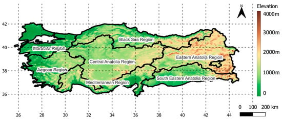
Figure 1.
Study area.
Rainfall and temperature patterns in Türkiye also present distinct features over the region. The eastern coast of the Black Sea region receives the highest amount of rainfall with over 2200 mm of annual rainfall, while central Anatolia in Türkiye receives approximately 400 mm of annual rainfall. Higher temperatures are experienced at the Mediterranean and Aegean coasts, the southern and southeastern parts of Türkiye, throughout the year compared to other parts of the country. The highest and lowest annual average temperatures are 21.3 °C (1962) and −0.2 °C (1960), respectively, which were measured in the Mediterranean Region (Hatay-İskenderun) and Eastern Anatolia Region (Kars-Sarıkamış) [29]. Overall, the annual average temperature is 13.9 °C and the precipitation value is 573.4 mm for the 1991–2020 period in Türkiye [58].
2.2. Data
2.2.1. ERA5-Land
In this study, ECMWF’s (ERA5-Land) dataset, a reanalyzing dataset for global climate and past weather [40], will be used as historical reference data. The ERA5-Land dataset provides data that are available for 2–3 months from 1950 to today. ERA5-Land provides hourly high-resolution information on surface variables. The data have a grid range of ~9 km [59], which is obtained as a result of reworking the terrain component of ERA5 climate re-analysis with a higher spatial resolution. Reanalyzing combines model data with observations collected from all over the world using the laws of physics to create a complete and consistent dataset globally. ERA5-Land is a customized variant of ERA5 data on land parts. The biggest difference from the original is that the horizontal resolution is presented as 0.1° × 0.1° instead of 0.25 × 0.25. This difference makes it possible to work on more precise scales. Temporal resolution is hourly, as in ERA5. This dataset will be used to downscale precipitation and temperature results from CMIP6 global climate models and to determine the performance of GCMs.
2.2.2. CMIP6 Global Climate Models
In this study, future climate projections will be taken from the most up to date CMIP6 global climate models. The aim of the CMIP is to better understand past, present, and future climate changes caused by natural variability or climate change due to changes in radiation coercion in a multi-model context. Using idealized experiments, with the participation of relevant investigative organizations around the world, in addition to long timescale changes, it investigates the predictability of the climate system at various time and space scales and makes predictions based on observed climate situations. An important goal of CMIP is to make multi-model outputs public in a standardized format.
The sixth edition of the CMIP, CMIP6, demonstrates better performance compared to its predecessor CMIP5 [31]. Determining the amount of natural or anthropogenic irradiation, the inclusion of aerosol, and land-use effects are some of the reasons behind the aforementioned performance [29,60,61,62].
To provide consistency and fair comparison a single ensemble member (named rninpnfn, where r is for realization, i is for initialization, p is for model physics, and f is for forcing) approach was used and the outputs of the GCMs were selected from the ensemble member of r1i1p1f1 as much as possible in this study.
The names of the GCM models and data availability (historical, SSP2-4.5, SSP5-8.5) of CMIP6 models for variables (precipitation (pr), daily maximum temperature (tasmax), and daily minimum temperature (tasmin)) are referred in the Table 1.

Table 1.
CMIP6 models employed in the study with their respective variable and scenario.
2.3. Methodology
2.3.1. Bias Correction of Climate Variables
Different techniques are widely used to downscale and reduce the consistent bias in the mean and standard deviation of coarse-resolution climate model datasets. The ERA5-Land datasets are used to bias correct and downscale the gridded CMIP6 climate model data to a target resolution of 0.1 × 0.1 degree (approximately 9 km). In this study, the QM, DQM, and QDM methods, which were proved to exhibit better performance with extremes, were used. Bias-correction analyses were performed using R software version 4.2.2.
Quantile Mapping
QM is one of the most common methods used in the correction of the consistent biases existing in gridded datasets [36,63,64,65,66]. This method is based on calibrating the CDF of the target data to the CDF of reference data (e.g., calibrate the climate model data CDF utilizing ERA5-Land CDF). The transfer function obtained during this calibration is used to correct biases in the future predictions of the climate model. Studies have shown that QM or CDF matching algorithms yield sufficient results for precipitation data [5,66]; Chen et al. [67] showed that QM yielded more successful results than average-based bias correction methods. The QM method is performed using the following equation:
where represents the climate model data at time , and and represent the CDF of the CMIP6 model and the reference data, respectively.
Detrended Quantile Mapping
The DQM was proposed by Cannon et al. [36] and, unlike quantile mapping, contains additional but limited information from climate model predictions in the form of the projected mean. The climate change signal from DQM will often pair with that of the underlying climate model, depending on how much extrapolation is still needed after detrending. While this holds true for the mean, it may be insufficient to prevent trend distortions at the extreme points of the distribution representing climate extremes.
In addition to quantitative mapping, the terms and given in this equation are the averages of the modeled historical period and the forecast period at time , respectively.
Quantile Delta Mapping
The quantile delta mapping technique was generated to correct the systematic biases while preserving the relative changes in the modeled quantiles of the variable under study [36]. The bias-corrected value was obtained using the reference data and the relative change term was obtained from the model data in the quantile delta mapping basic equation [68,69]. The difference in this method from the trendless quantile mapping method is that all modeled quantiles are taken into account, not just the modeled mean.
In these equations, represents the bias-corrected historical period data, and represents the relative change in the model data over the historical and forecast periods [36,68,69].
2.3.2. Performance Evaluation for Bias Corrected Data
Kolmogorov–Smirnov (K-S) Test
The performance of the bias correction techniques was first validated by selected historical precipitation and temperature extreme indices. The 1961–1990 period was chosen as the calibration period by using references for the QM, DQM, and QDM algorithms, and then extreme indices were calculated over 1991–2014 for the validation period. For each ERA5-Land grid, indices calculated before and after bias correction are compared by using the Kolmogorov–Smirnov (K-S) test, which is based on the comparison of distributions between the historical reference (ERA5-Land) and model data with and without bias correction. The null hypothesis postulates that the two samples are derived from an identical distribution. A diagnostic evaluation is performed at a grid cell to determine if the model meets the criteria. The diagnostic test is considered successful if the null hypothesis is not rejected, meaning that none of the quantiles of the modeled distribution fall beyond the 99% confidence interval of the historical reference quantiles, as indicated by studies conducted by Bürger et al. [70] and Cannon et al. [36].
Multi-Model Ensemble Weighted Average
The multi-model ensemble average (MMEA) is a commonly used approach in climate modeling studies to handle the uncertainties and biases stemming from GCMs [71,72]. Although there is no scientific consensus for determining the number of GCMs involved in analyses, studies reveal that the first 3 to 10 GCMs are commonly used in the multi-model ensemble average (MMEA) [72]. However, some studies prefer to incorporate all available GCMs without the need to rank [73], which can result in the poor performance of MMEA because of the insufficient representation of the orography or boundary structure [29]. Moreover, the computational load increases with the increasing number of GCM members in climate modelling studies when downscaling is applied. On the other hand, reasonable weighting can make a considerable contribution to reducing the uncertainties derived by the inter-model differences, to loss of signal and for projecting future changes. Consequently, it is important to determine enough multi-model ensemble (MME) members in this approach. Here, GCMs were selected for precipitation and temperature separately, based on the multi-model ensemble weighted average, which were obtained based on the performance evaluation analyses in this study. The models were assessed to determine the skill in simulating climate extremes by the K-S test. The multi-model weighted ensemble average is calculated by taking the average of the predicted values from each model, weighted by the skill of each model in reproducing historical reference data. In other words, models that are more accurate in reproducing reference data are given more weight in the ensemble average, while less accurate models are given less weight. While the weighting can be based on a variety of factors, in this study, the model’s ability to simulate extreme features of interest was employed. The weighted average of the model outputs was then used to obtain the ensemble average future results. All analyses were performed using R software version 4.2.2 (R Foundation for Statistical Computing, Vienna, Austria).
2.3.3. Expert Team on Sector-Specific Climate Indices (ET-SCI)
The WMO formed an expert team on ET-SCI for developing extremes indices to analyze the impact of climate extremes that are relevant to different sectors [24,26,74]). These sector-specific extreme indices can be categorized into four groups: (1) absolute indices, (2) threshold indices, (3) duration indices, and (4) percentile indices [75]. Absolute indices represent a maximum or minimum value within a period while threshold indices count the number of days when a temperature or precipitation value falls above or below a selected threshold. Duration indices signify a warm, dry, or cold spell, and percentile indices describe the rate of exceedance of a percentile, which is calculated based on a priorly defined baseline period.
Table 2 summarizes the chosen 12 extreme temperature and 12 extreme precipitation indices that are computed in this study. Indices were calculated for the historical period using ERA5-Land, and for the future period using two SSP scenarios: selected and ensemble GCMs. For clarity, the indices in Table 2 were grouped under five broad categories: i. percentile-based indices, ii. absolute indices, iii. threshold indices, iv. duration indices, and v. other indices. Indices are derived from daily maximum and minimum of near-surface temperature and daily precipitation data (TX, TN, and PR).

Table 2.
The set of selected Climpact indices and their corresponding information [24].
Climpact software and R software (4.2.2) have been used to calculate the extreme temperature and precipitation indices [24]. A flowchart that includes methodological details regarding this study is shown in Figure 2.
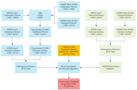
Figure 2.
Outline of bias correction steps with applied methods.
3. Results
3.1. Performance and Validation of the Bias Correction Methods
The performance of the bias correction methods is first evaluated by applying the bias correction algorithms to daily historical GCM outputs, deriving the 24 ET-SCI indices from raw and bias-corrected data, and then checking to see if distributions of the 24 ET-SCI precipitation and temperature extreme indices are consistent with historical reference data-driven indices.
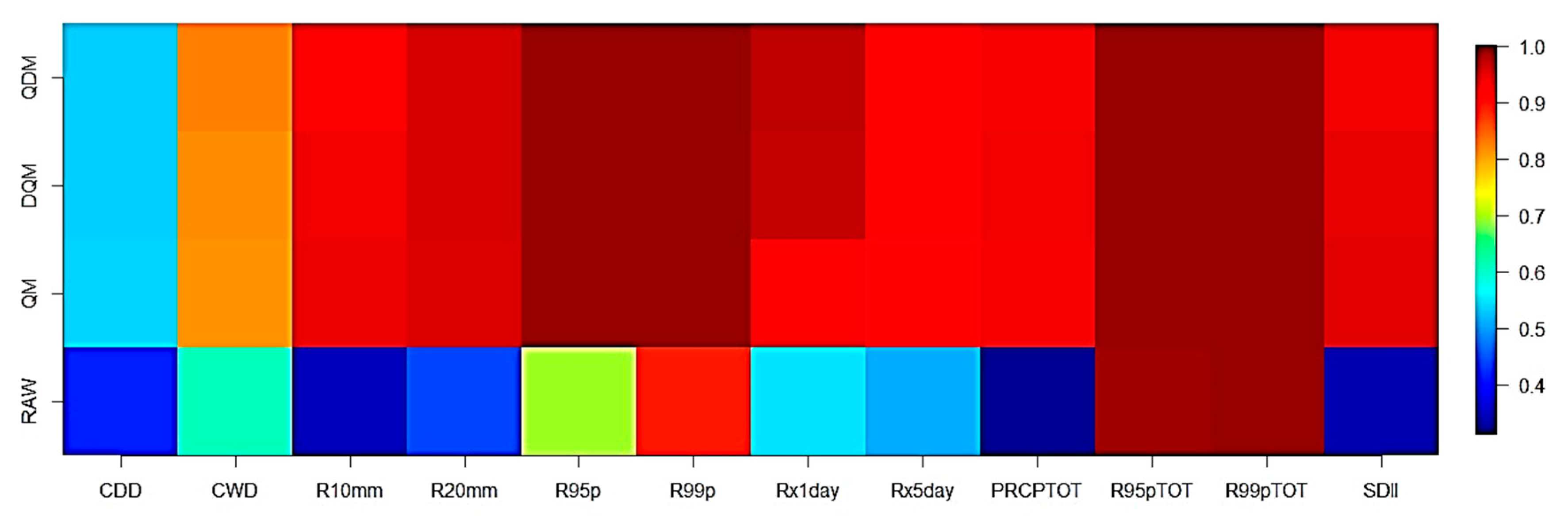
The distributions of the ET-SCI indices, both pre- and post-bias correction, are compared to the distributions derived from historical reference data using the K-S test at a 0.01 significance level for each of the 9135 ERA5 Land grid cells in Turkey and approximately 40 models [36,70]. Subsequently, the proportion of grid cells passing K-S tests for each index was calculated throughout Türkiye for all models, shown in Figure 3 and Figure 4 for precipitation and temperature indices, respectively. In these figures, increasing values from 0.00 (indicates no agreement) to 1.00 (indicates perfect agreement) demonstrate better performance. For instance, the Rx1day index is calculated for 43 models in every single ERA5-Land grid in Türkiye, then the K-S test is applied for every single index value, and the proportion of the passing values are 0.546, 0.938, 0.973, and 0.975, respectively, for the raw GCM, QM, DQM, and QDM methods.

Figure 3.
Proportion of raw and downscaled grid cells passing local K-S diagnostic tests for each ET-SCI precipitation index over the 1991–2014 independent validation period.

Figure 4.
Proportion of raw and downscaled grid cells passing local K-S diagnostic tests for each ET-SCI temperature index over the independent 1991–2014 validation period.
K-S test results for the historical period are summarized in Figure 3 and Figure 4 as heat maps for both the raw GCM and bias-corrected output-driven indices. Over the validation period, all three methods outperformed the raw GCM outputs according to the K-S test for the 24 ET-SCI indices. Every single cell in Figure 3 and Figure 4 consists of the entire Türkiye and all models (~9135 grid × 40+ models). Among the bias correction algorithms, the QDM exhibits slightly better performance than QM and DQM for the precipitation-based extreme indices while we could not find a significantly superior method for the temperature-based extreme indices. For instance, for the PRCPTOT, total precipitation indices, the raw GCM performance is 0.31 (31% of grids have consistent raw GCM and ERA5 Land CDFs during the independent validation period based on the K-S test at a 0.01 significance level), while this ratio increases to approximately 0.94 for all three bias correction methods (Figure 3). Considering the temperature, 10 out of 12 indices revealed considerably better performance with their bias-corrected values. Raw CSDI and WSDI indices on the other hand did not exhibit any improvement compared to their bias-corrected values, 99% and 98%, respectively (Figure 4).
The three quantile mapping algorithms were evaluated based on the reduction in the K-S test statistic (D), which is the maximum difference between CDFs. The success rates of the algorithms are presented in Figure 3 and Figure 4. Although these algorithms were applied to daily GCM data, the distributions of the ET-SCI indices were effectively corrected by the quantile mapping approaches. The bias correction algorithms demonstrated stable validation performance and showed remarkable improvements across variables. Generally, all three algorithms proved to be robust and capable of correcting substantial systematic biases in GCM representations of the ET-SCI indices throughout the historical simulation period. While the methods were indistinguishable in terms of performance, we opted to proceed with QDM, as it is consistent with and known to preserve the relative trends projected by GCMs in the literature [36].
3.2. Performance of the GCM Models
Prior to evaluating future climate projections, it is common practice to assess the accuracy of historical simulations produced by GCMs against reference data [5,76]. The performance of the models was determined by deriving the 24 ET-SCI indices from daily historical raw GCM outputs and then checking to see whether or not distributions of the 24 ET-SCI values are consistent with the relevant index values obtained utilizing ERA5-Land as a reference dataset. The same methodology mentioned above was also used for the model performance evaluation. Moreover, four indices (R95pTOT and R99pTOT for precipitation, WSDI and CSDI for temperature) that have a significantly lower coefficient of variance have been excluded from the performance analyses due to a misleading increase in model weights that will be used in the weighted multi-model ensemble.
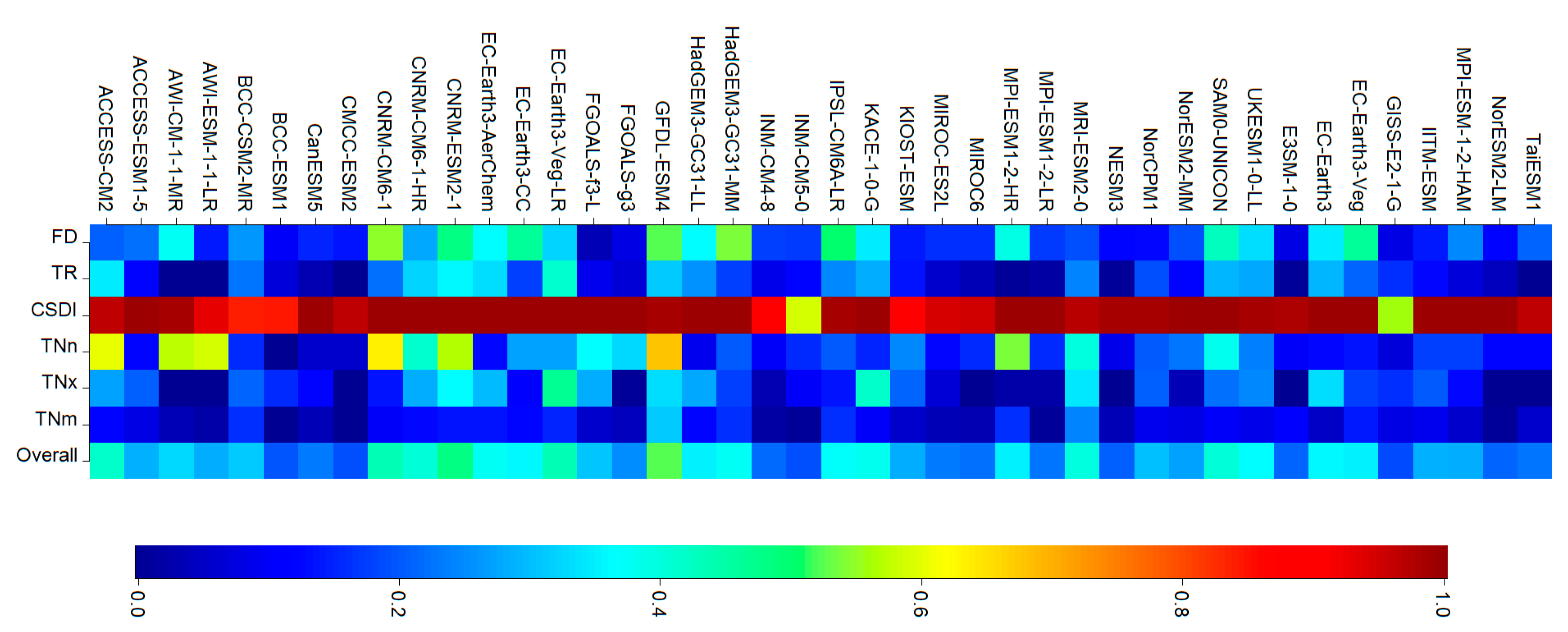
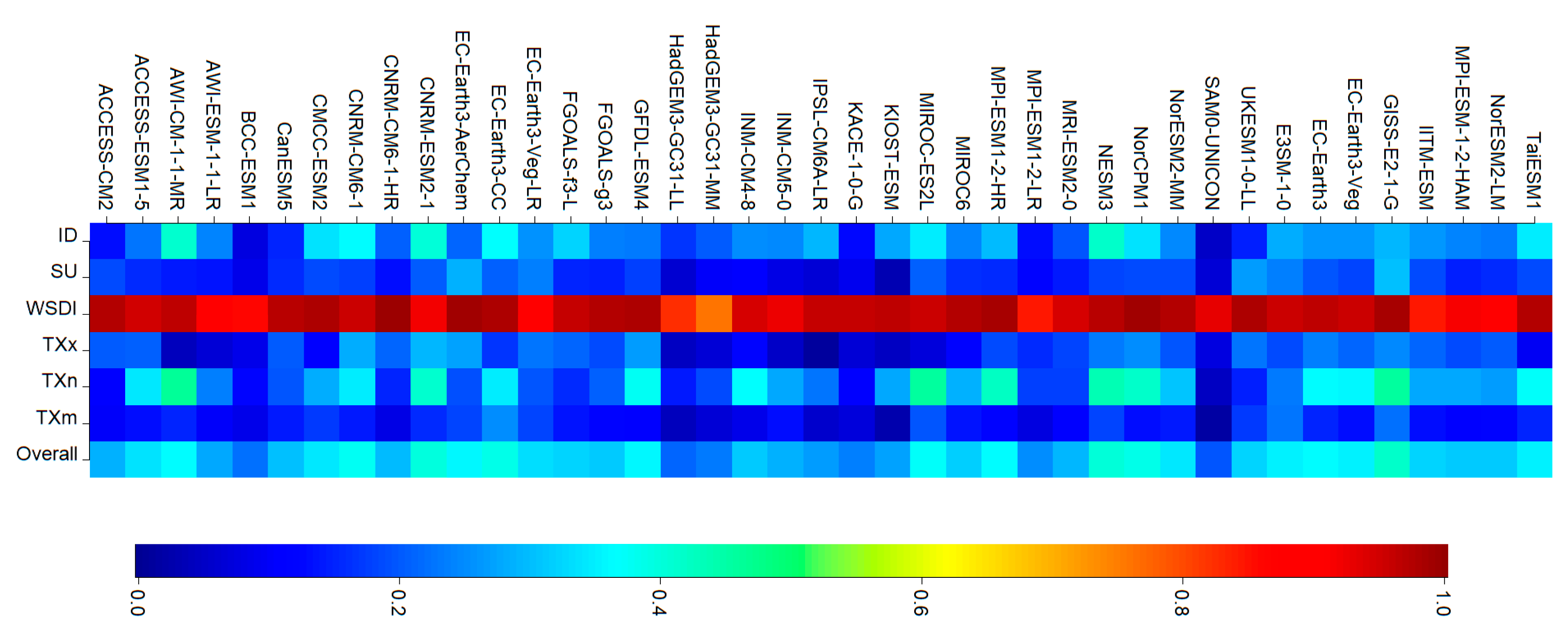
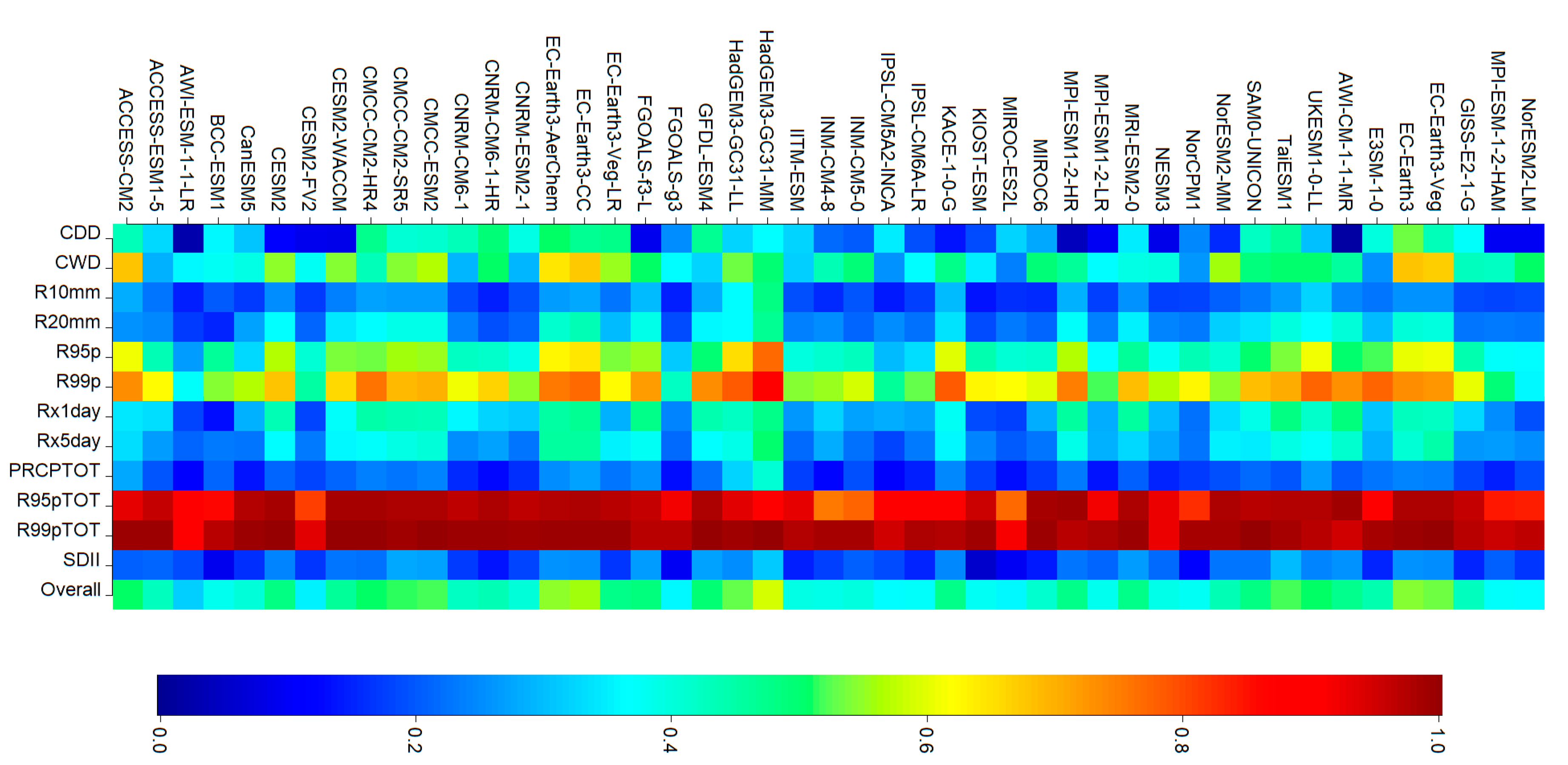
Figure 5, Figure 6 and Figure 7 illustrate the ability of CMIP6 models to simulate the near-surface (air) temperature and precipitation in Türkiye from 1961 to 2014. As a whole, precipitation-based index simulations of CMIP6 models outperform temperature-based simulations.
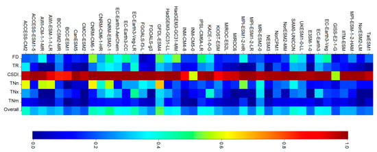
Figure 5.
Percentage of historical raw CMIP6 models passing K-S test for each minimum temperature index.
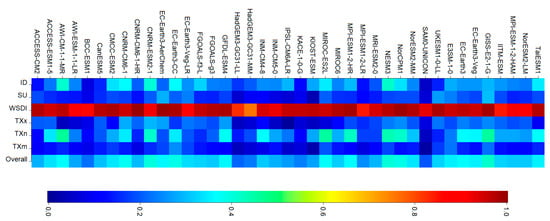
Figure 6.
Percentage of historical raw CMIP6 models passing K-S test for each maximum temperature index.
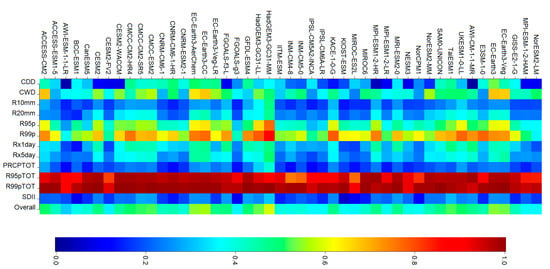
Figure 7.
Percentage of historical raw CMIP6 models passing K-S test for each precipitation index.
Among CMIP6 models, the HadGEM and EC-Earth model family members have better precipitation simulations, having the highest 6 ranking among 47 models (Figure 7). Furthermore, EC-Earth models also perform better than other CMIP6 models in terms of minimum temperature indices. On the other hand, there is not a significantly better model family among the CMIP6 models for the maximum temperature-based indices; instead, the top performer model is HadGEM3-GC31-MM, which is also the top model for the precipitation. According to the results of the K-S test, SAM0-UNICON among the CMIP6 models provides the best historical performance for temperature, while HadGEM3-GC31-MM provides the best performance for precipitation.
According to the latest IPCC report (AR6 report), the likely range of equilibrium climate sensitivity (ECS; representing the expected global warming following doubling of the atmospheric CO2 compared to its pre-industrial levels) was estimated to be 2.5–4 °C. The range of 2.3–4.7 °C was estimated with a 5–95% probability [77]. It should be noted that some of the high-performer models, such as HadGEM family members and EC-Earth3-CC, have higher equilibrium climate sensitivity (ECS) values than the likely ECS range of 2.5–4 °C reported by the IPCC AR6 report [31]. Although these high-sensitivity models do not fall within the likely range, because of their high performance in the historical period, they are not excluded from the mean ensemble. Even though the ECS of some of the CMIP6 models are out of that likely range, development on the cloud–aerosol interaction and their climate feedbacks could make the climate system highly sensitive and those higher ECS values plausible [78]. Nevertheless, it is important to evaluate the consequences of those less likely but high-risk CMIP6 future climate projections as also stated by Bayar et al. [31].
In Türkiye, a limited number of studies have used the CMIP6 projections and analyzed their performance up until now. Bagcaci et al.’s [29] study is one of the frontiers and is highly regarded among the others that have evaluated the CMIP5 and CMIP6 performance in Türkiye. The model performance results of this study reveal similar findings to Bagcaci et al. [29] in terms of the list of models that have the highest performances, even though the number of models examined in that study is 31 while this study investigates over 40 models. This difference is one of the reasons for the model performance results of both studies together with the temporal resolution, which is monthly in the aforementioned study.
3.3. Behavior of Indices
The changes in indices between historical and future periods were examined under two main headings based on precipitation and temperature. Three different periods were examined, including the near (2015–2040), medium (2041–2070), and far (2071–2100) future, with 30-year periods for both SSP2-4.5 and SSP5-8.5 scenarios. The results obtained from the performance-based weighted average model ensemble are presented. In order to make both the analysis and interpretation of the obtained results easier, changes in indices were shown for seven geographical regions in Türkiye and for all of Türkiye.
3.3.1. Extreme Precipitation Indices (EPI)
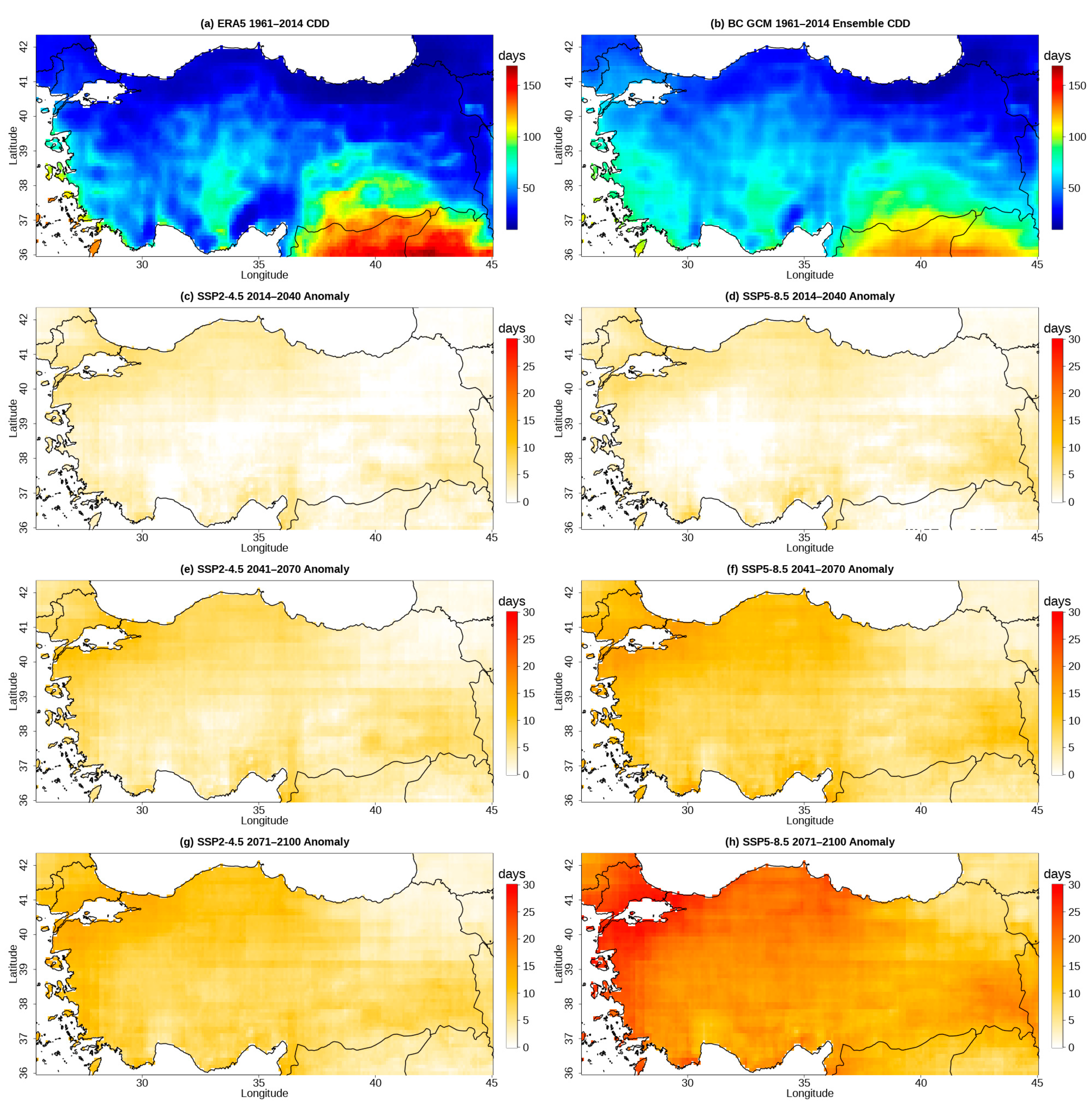
The results for six extreme precipitation indices are given for different time periods and two projection scenarios in Table 3 (CDD, CWD, R10 mm, R20 mm, R95p, R99p) and the spatial distribution of CDD for 1961–2014 and 2015–2100 under the two scenarios is also shown in Figure 8.

Table 3.
Values of the six EPIs in the seven sub-regions (Aegean (Aeg.), Central Anatolia (Cen. Ana), Black Sea (Blck.), Eastern Anatolia (East. Ana.), Mediterranean (Med.), Southeastern Anatolia (Se. Ana.), Marmara (Mar.)), and Türkiye under two scenarios (SSP2-4.5 and SSP5-8.5) for historical and three future periods (15–40, 41–70, 71–100).
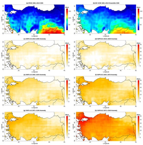
Figure 8.
Spatial distributions of the CDD during historical period (a,b) and differences from the historical period for 2015–2040 (c,d), 2041–2070 (e,f), and 2071–2100 (g,h) under the SSP2-4.5 and SSP5-8.5.
The CDD index in Table 3 shows the maximum consecutive number of days with daily precipitation below 1 mm where higher values indicate longer dry seasons. For the historical period, the highest CDD values are obtained for Southeastern Anatolia and Aegean regions while the lowest values are observed in the Black Sea and Eastern Anatolia regions (Table 3 and Figure 8a,b). When Figure 8a,b are compared, it is shown that regional patterns are consistent with ERA5-Land references with a slight bias. For Türkiye overall, the mean value for the historical period is calculated as 53.8 days. Considering Figure 8, a positive trend is observed in all regions where the difference from the historical period becomes more distinct during the mid- and late century for both scenarios.
While the highest CDD value is observed for Southeastern Anatolia and Aegean regions under the SSP5-8.5 scenario during the late century with 96.3 and 85.4 days, respectively (Table 3), the highest increase is observed for the Marmara region for the same scenario and period where the CDD increased from 49.6 to 74.4 days (Figure 8h). These results indicate the increasing possibility of dry periods for all of Türkiye.
CWD in Table 3 shows the maximum consecutive number of days with daily precipitation above 1 mm where higher values indicate longer precipitation windows. For the historical period, the CWD values range between 8.2 and 13.4 days, where upper and lower boundaries belong to the Black Sea and the Aegean regions, respectively, while the mean for all of Türkiye is calculated as 10.1 days (Table 3). A slight decrease is observed in all regions for both emission scenarios during the projection period; however, SSP5-8.5 (8.7 days) projects a slightly lower value than SSP2-4.5 (9.5 days). Although the highest decrease is observed for the Mediterranean region (from 10 days to 8 days), it is not possible to mention a sharp change in any of the regions (Table 3). Compared to the changes in CDD, the CWD future change is less in Türkiye. However, when both indices are considered together increased CDD and decreased CWD values indicate drought conditions will intensify in the future.
R10 mm shows the number of days with a total precipitation higher or equal to 10 mm. A higher value indicates heavy precipitation is more common in the region and lower values indicate that these events are scarcer. For the historical period, the lowest value is calculated in Central Anatolia with 10.8 days and the highest value is obtained for the Black Sea region with 28.9 days. The mean for all of Türkiye is found to be 19.7 days (Table 3).
The SSP2-4.5 scenario R10 mm index shows different trends for different regions. While the values decrease over the Aegean, Mediterranean, and Southeastern Anatolia regions, an increase is expected in the Eastern Anatolia and Black Sea. Marmara and Central Anatolia show no remarkable change. Alternatively, the SSP5-8.5 scenario predicts different trends and more significant changes. While the Aegean, Mediterranean, Southeastern Anatolia, and Marmara regions show stronger decreasing trends, the values for other regions do not change significantly from the historical period (Table 3). The temperature, GCM-based variations, and changes in precipitation amount and intensity can be shown as causes of changes in R10 mm values. In addition, the effect of greenhouse gas emissions and land use changes, which are the leading anthropogenic factors, cannot be ignored.
The R20 mm in Table 3 indicates the number of days for daily precipitation exceeding 20 mm. Comparison between R10 mm and R20 mm values can also give an idea about the frequency and severity of heavy rainfall events in this region and periods. During the historical period, the highest R20 mm values were observed in the Mediterranean (8.1 days) and the lowest values in the Central Anatolian region (1.5 days). While R20 mm values generally increase in the projection periods, the highest values are expected in the Black Sea and Southeastern Anatolia regions (Table 3). An increase in R20 mm values may indicate an increase in very heavy rainfall events and may have adverse effects such as flooding and soil erosion in areas exposed to this increase.
As seen in Table 3, the R20 mm values in the SSP5-8.5 scenario are generally higher than those in the SSP2-4.5 scenario (Table 3), suggesting that extreme precipitation events may occur more frequently and severely under high emission scenarios in the future. Compared to the R10 mm results, the regional distribution of the R20 mm values appears similar. However, it should be noted that the R20 mm values for Eastern Anatolia and Black Sea regions are relatively higher than other regions. When the historical period is compared with future scenarios (Table 3), the relatively higher R20 mm values for the SSP2-4.5 and SSP5-8.5 scenarios suggest the possibility of an increase in heavy precipitation in the future. However, it is important to note that the magnitude of the increase varies by region and scenario. In different regions of Türkiye and in different scenarios, there is generally a decreasing trend for R10 mm and an increasing trend for R20 mm, indicating a decrease in the frequency of heavy rains but an increase in very heavy rains.
The R95p in Table 3 represents the annual total precipitation when the daily precipitation is above the 95th percentile. The 95th percentile was calculated with respect to the historical period and kept constant for all projection periods. When we compare the values between different time periods and regions, it can be seen that under all scenarios, an increase in extreme precipitation is expected in most of the regions in Türkiye based on the results of the R95p index. This increase is more evident in regions other than the Aegean and Mediterranean regions. Especially in the Black Sea and Eastern Anatolia regions, increases of up to 36% and 40% are expected at the end of the century. The results in the Aegean and Mediterranean regions do not indicate a significant increase or decrease in this index. On the other hand, while a general increase is expected in both the GCM SSP2-4.5 and GCM SSP5-8.5 scenarios in the near, medium, and far future, there is no significant difference between the scenarios when Türkiye averages are compared. When the differences between the regions in Türkiye are examined, it is seen that there are serious differences between the regions (Table 3). For example, when the Black Sea region (189.7 mm) is compared to Central Anatolia (89.4 mm) in the historical period, a difference of almost 100 mm is observed, and when the end of the century is reached, these differences are seen to increase even more under the SSP5-8.5 scenario (369.8 mm–111.7 mm). This can be seen as an indication that the magnitude of heavy precipitation events in the Black Sea region today and in the future is greater than in Central Anatolia and the deviation between these two regions will further increase.
The R99p heavy rainfall index in Table 3. shows the expected changes in the frequency of extreme rainfall events in different regions of Türkiye in different time periods. During the observation period, the highest R99p index values were observed in the Black Sea (54.5 mm) and Mediterranean (52.7 mm) regions, while the lowest values were observed in the Central Anatolia (25.9 mm) region. Under the SSP2-4.5 and SSP5-8.5 scenarios, the R99p index starts to increase in all regions compared to the observation period. The magnitude of these increases is particularly high in the Black Sea, Eastern Anatolia and Southeastern Anatolia regions. This indicates a significant increase in the frequency of extreme heavy rainfall events in these regions. In general, the results indicate that the frequency of extreme precipitation events in different regions of Türkiye may change in the future, but it will inevitably increase, especially in the distant future.
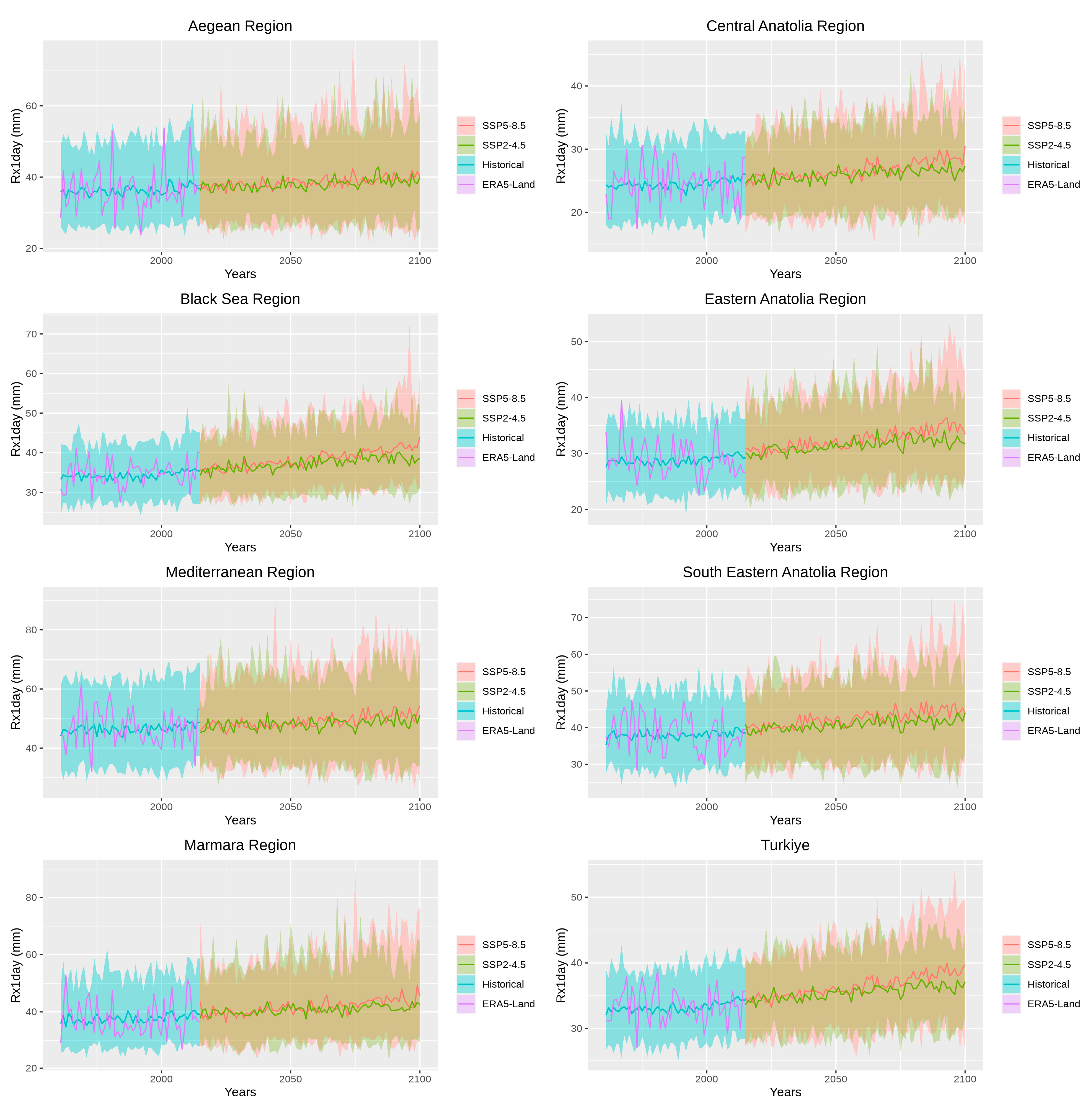
The results for six extreme precipitation indices are given for different time periods and two projection scenarios in Table 4 (Rx1day, Rx5day, PRCPTOT, R95pTOT, R99pTOT, and SDII). Temporal variation of Rx1day in Türkiye and for the sub-regions were represented for 1961–2100 with two scenarios in Figure 9.

Table 4.
Values of the six EPIs in the seven sub-regions and Türkiye under the two scenarios (SSP2-4.5 and SSP5-8.5) for historical and three future periods (15–40, 41–70, 71–100).
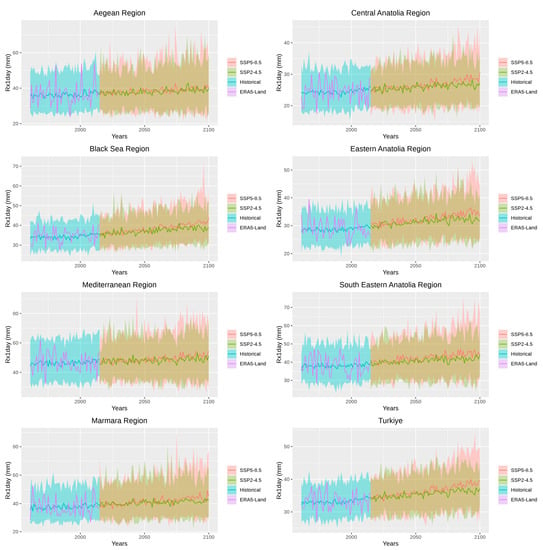
Figure 9.
Time series of Rx1day over historical period and 2015–2100 under the two scenarios in the seven sub-regions and across Türkiye. The top and bottom boundaries of the shaded area are the 97.5th and 2.5th percentiles of the GCMs.
The Rx1day in Table 4 shows the maximum daily precipitation that occurred in a given year. According to the table, the average historical value of the Rx1day index for Türkiye is 33.2 mm. When the spatial variation of historical values of the Rx1day index is examined, it shows that the highest values are generally recorded in the Mediterranean region and the lowest values are recorded in the Central Anatolia and Eastern Anatolia regions (Table 4). The projections show that the index values are expected to increase for all regions and scenarios in the future (Figure 9), and the highest increase is expected in the Black Sea and Eastern Anatolia regions for the 2071–2100 period within the scope of the SSP5-8.5 scenario (Table 4). The values obtained from the GCM simulations indicate that the frequency and intensity of extreme precipitation events may increase in the future, especially under the SSP5-8.5 scenarios. When Figure 9 is investigated, it should also be noted that, in addition to the increase in ensemble means, the span of the 95% confidence interval of models also widens when moved from the historical period to the end of the century. This suggests an increase in the uncertainty and intensity of extreme events. While interpreting these changes, it should be kept in mind that the projections are subject to the uncertainties and limitations of GCM simulations, and the impact of complex topographic elements of a country such as Türkiye on precipitation characteristics cannot be denied on a regional basis.
While Rx1day shows the maximum precipitation for the daily scale, Rx5day in Table 4 demonstrates 5 days of cumulative maximum precipitation for the year of interest. Considering the Rx5day extreme precipitation index values, the observation data show that the Mediterranean region has the highest average with 98.3 mm, while Central Anatolia has the lowest average with 50.5 mm. For all projection periods, a general trend of increase in Rx5day extreme precipitation index values emerges in all regions (Table 4). In the late century, average heavy precipitation increases overall are expected across Türkiye. This increase is predicted to be 5.5% according to the SPP 2-4.5 and 7% according to SSP5-8.5, but again, the difference between regions should not be ignored in the evaluations to be made. Despite the 13% increase seen in the Black Sea region, no significant trend was observed in the Mediterranean and Aegean regions in the same period. However, it should be noted that even though there has been no increase, the values of the Mediterranean region are still much higher than Türkiye’s average. The highest average 5-day excessive precipitation increase rates are observed in the Black Sea and Eastern Anatolia regions with 86.4 mm (13%) and 74.9 mm (12%) in the GCM SSP5-8.5 71–100 period (Table 4).
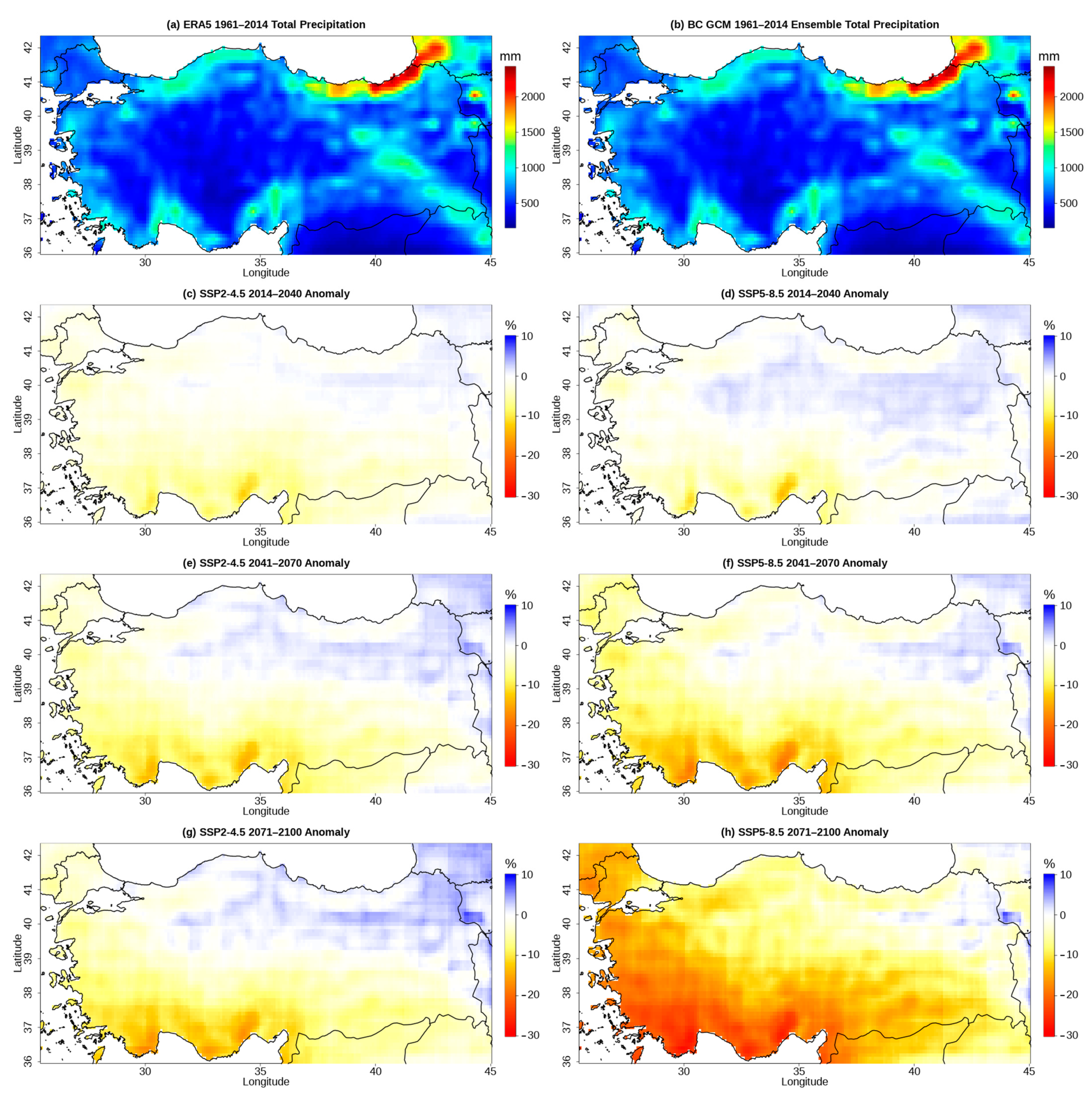
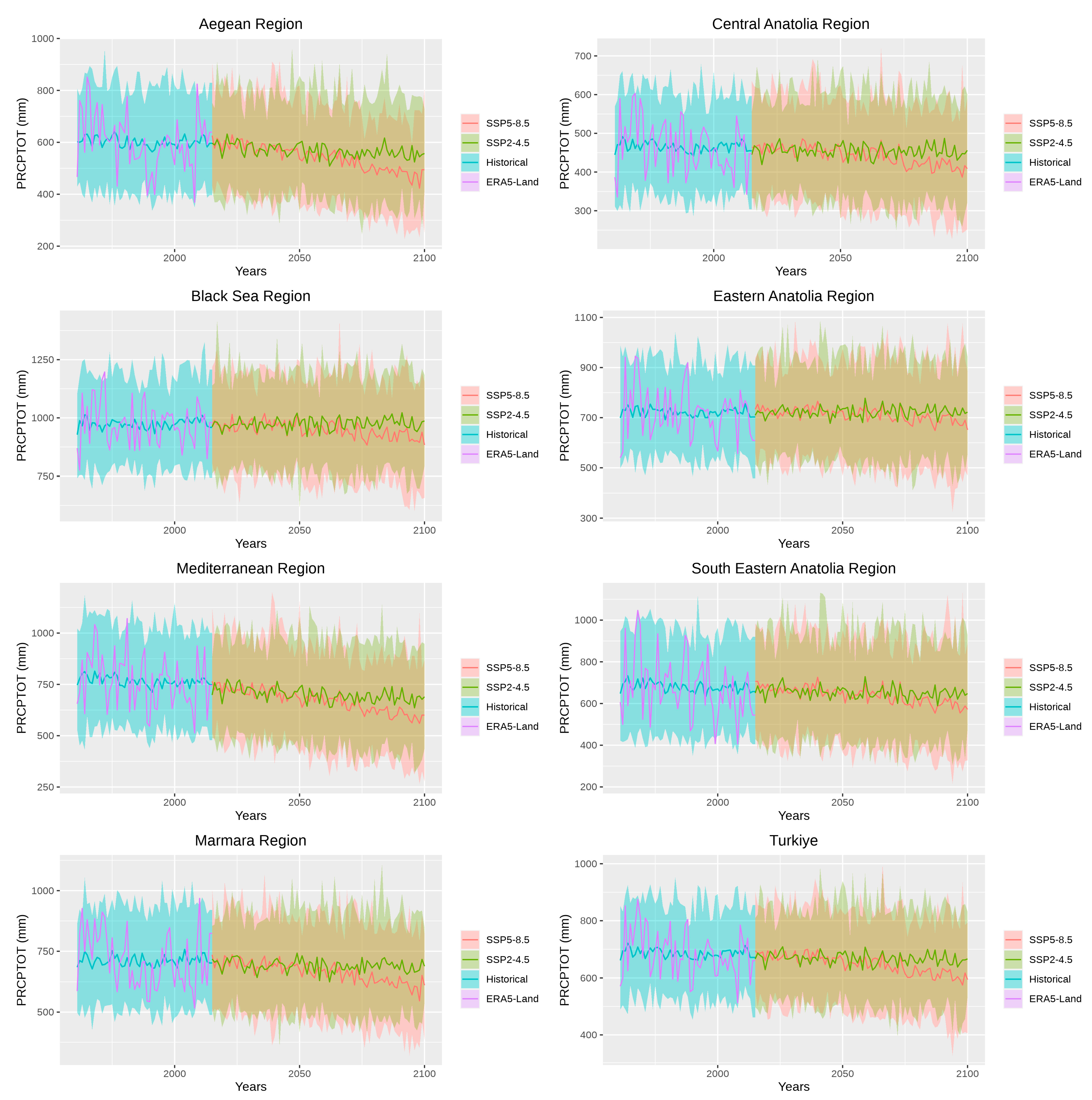
The PRCPTOT index in Table 4 gives information about the total amount of precipitation in millimeters at different periods and regions in Türkiye. Also, spatial and temporal distributions of PRCPTOT for 1961–2014 and 2015–2100 under the two scenarios are shown in Figure 10 and Figure 11 respectively. For the historical data, the highest total precipitation is observed in the Black Sea region (973.8 mm), while the lowest precipitation is observed in the Central Anatolia region (465.5 mm). On the other hand, the average total amount of precipitation in Türkiye is 686.1 mm (Table 4). The SSP2-4.5 scenario predicts a decrease in total precipitation for all regions except the Black Sea and Eastern Anatolia, while it shows a slight increase in total precipitation in the Black Sea.
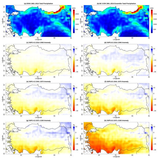
Figure 10.
Spatial distributions of the PRCPTOT (a,b) during historical period and percent differences from the historical period for 2015–2040 (c,d), 2041–2070 (e,f), 2071–2100 (g,h) under the SSP2-4.5 and SSP5-8.5.
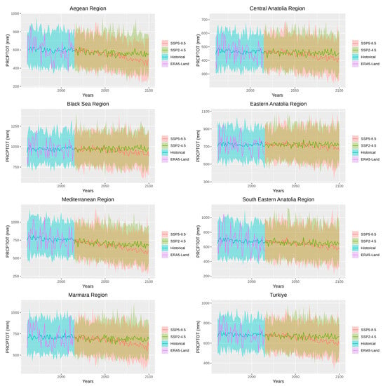
Figure 11.
Time series of PRCPTOT over historical period and 2015–2100 under the two scenarios in the seven sub-regions and across Türkiye. The top and bottom boundaries of shaded area are the 97.5th and 2.5th percentiles of the GCMs.
Figure 10 shows the greatest decrease in total precipitation in the Mediterranean region among the regions, where the total precipitation decreased from 766.3 mm to 684.4 mm in the SSP2-4.5 late-century period (Table 4). The SSP5-8.5 scenario also predicts a reduction in total precipitation for all regions, and the reduction in the total precipitation is generally larger compared to the SSP2-4.5 scenario (Table 4 and Figure 10). Similarly, the greatest decrease in total precipitation is predicted for the Mediterranean region, where it dropped from 766.3 to 613.9 mm in the SSP5-8.5 late-century period. Additionally, a decrease of more than 100 mm is expected in the Aegean region. It is also estimated that the whole of Türkiye will have an average total precipitation of 615.6 mm, corresponding to a decrease of 70 mm during the SSP5-8.5 late-century period. The time series in Figure 11 shows that regional means for both scenarios have similar trends up to the late century (2071–2100). However, after that point, the scenarios display a diverging trend wherein SSP5-8.5 predicts significant drops in most of the regions. The difference predicted between the two scenarios is relatively smaller for Eastern and South Eastern Anatolia regions. In general, projections show that the total precipitation in Türkiye is predicted to decrease in the future, especially in late periods; however, it should also be noted that Figure 10g suggests that almost half of the country might have no significant trend or slight increases by the end of the century according to the SSP2-4.5 scenario (Figure 10 and Figure 11).
The R95pTOT index (fourth in Table 4) is found by dividing the R95p index by the PRCPTOT index. In other words, it gives the ratio of precipitation above the 95th percentile to the total precipitation. When the values are examined, it can be said that for the observation period, all regions have values close to Türkiye’s average. However, the highest R95pTOT value in the historical period was calculated in the Mediterranean (23%) region. It can be seen from the table that there is a general upward trend in this index as well as in the R95p value. When Türkiye averages are examined, it is seen that this increase is close to 30% for the SSP2-4.5 scenario at the end of the century, and 43% for the SSP5-8.5 scenario in the same period. In summary, although the R95pTOT extreme precipitation index values differ between different regions and time periods, the general trend is that the values increase over time and reach the highest values observed in the GCM SSP5-8.5 2071–2100 period.
The R99pTOT in Table 4 shows the ratio of precipitation above the 99th percentile to total precipitation, similar to R95pTOT. When the values are examined, an R99pTOT value of 5.8% is seen for the Türkiye average during the observation period. The R99pTot index differs from the R95pTot index with its increase rates. For the 2071–2100 period, an 8.9% R99pTOT value is obtained for Türkiye in the SSP2-4.5 scenario, while this value is 11.1% for the SSP5-8.5 scenario (Table 4). When both values in the table are compared with the observation period, the expected increase at the end of the century for the SSP2-4.5 scenario is over 50%, while this increase prediction approaches 100% for the SSP5-8.5 scenario. Although values vary between regions, the general trend is that there is an increase in R99pTOT as the time period increases under both the SSP2-4.5 and SSP5-8.5 scenarios. This indicates that the percentage of extreme precipitation events in total precipitation will increase in the future. Especially in the SSP85 scenario, the Black Sea, Eastern Anatolia, and Southeastern Anatolia regions attract attention with their increase rates for the end of the century.
As the final precipitation index in Table 4, the SDII index is obtained by dividing the total precipitation by the number of rainy days (PR >= 1 mm). The intensity values in Table 4 show that the historical mean SDII varies between 4.9 and 7.5 mm in different regions of Türkiye, where the highest-intensity values are observed in the Mediterranean and Southeastern Anatolia regions and the lowest values are found in the Central Anatolia region. Future projections based on the SSP2-4.5 and SSP5-8.5 scenarios predict that SDII may increase in all regions and time periods in the future, with the largest increases in the SSP5-8.5 scenario. However, while the magnitude of the increases in SDII varies according to different regions, it is expected to reach its highest values in the Mediterranean, Southeastern Anatolia, Aegean, and Marmara regions. When these changes are evaluated together with the PRCPTOT and Rx1day indices, it can be concluded there is a decrease in the number of rainy days and an increase in extreme precipitation resulting from higher intensity.
3.3.2. Extreme Temperature Indices (ETI)
Minimum Temperature Indices
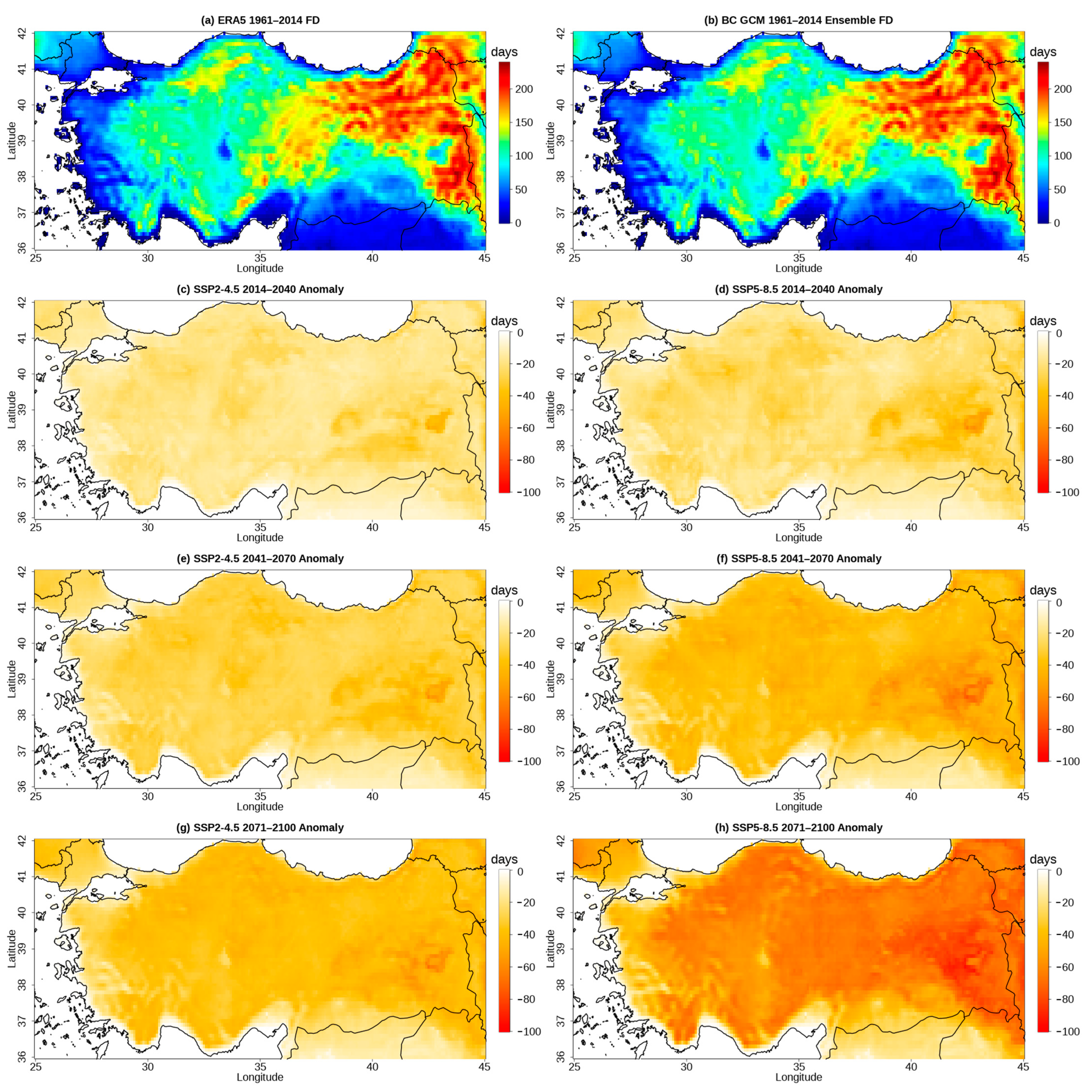
The results for six extreme minimum temperature indices are given for different time periods and two projection scenarios in Table 5 (FD, TR, CSDI, TNn, TNx, TNm), and the spatial distribution of FD is represented for 1961–2014 and 2015–2100 under the two scenarios in Figure 12.

Table 5.
Values of the six ETIs in the seven sub-regions and Türkiye under the two scenarios (SSP2-4.5 and SSP5-8.5) for historical and three future periods (15–40, 41–70, 71–100).
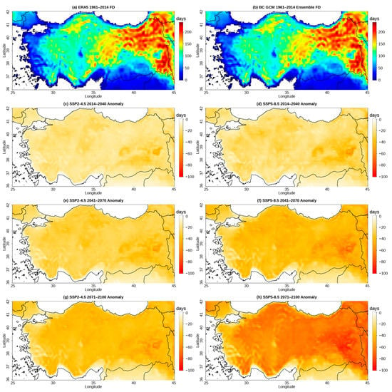
Figure 12.
Spatial distributions of the FD during historical period (a,b) and differences from the historical period for 2015–2040 (c,d), 2041–2070 (e,f), and 2071–2100 (g,h) under the SSP2-4.5 and SSP5-8.5.
The FD index in Table 5 shows the total number of days with a minimum temperature below zero in a year. As can be seen in Table 5., the FD index takes its greatest values during the historical period. In this period, the Eastern Anatolia Region comes first with 162.6 days. While Aegean, Mediterranean, Marmara, and Southeastern Anatolia regions were below Türkiye’s average (105.1 days), Marmara has the lowest value (49.1). Under the GCM SSP2-4.5 scenario, it is seen that the FD index is predicted to decrease in all seven regions of Türkiye compared to the observation period. Similarly, a decrease is predicted in all seven regions of Türkiye under the SSP5-8.5 scenario, but the magnitude of the decrease is generally larger than in the GCM SSP2-4.5 scenario. When the decreases are considered proportionally, it is seen that the highest decreases are predicted for Marmara (75%), Aegean (65%), and Southeastern Anatolia (65%) regions. In terms of absolute change, the decrease in Eastern Anatolia, where the FD dropped from 162.6 to 91.4 days (Table 5), is the most affected region. These results indicate that in both scenarios, the frequency and duration of FD in Türkiye are likely to decrease over the century, but the rate of decline will be sensitive to future scenario changes (Figure 12).
The TR index is the number of days when the minimum temperature is above 25 °C in a year. In Table 5, it is possible to see that the TR Index values have increased over time for all regions and scenarios, and accordingly, it can be said that the risk of extreme temperature has increased. When analyzed regionally, although the highest rate of increase is seen in the Central Anatolia, Black Sea and Eastern Anatolia regions, the increases on a daily basis in these regions are mostly in the Marmara, Aegean, Mediterranean and Southeastern Anatolia regions. The average for Türkiye, on the other hand, increases from 11.7 days to 69.6 days by the end of the century, according to the SSP5-8.5 scenario.
As the CSDI index values show in Table 5, a lower CSDI value indicates that cold events have a shorter duration, while a higher value indicates events that last longer. Overall, the duration of cold events is expected to decrease in all regions compared to the observation period. In particular, the values of the GCM SSP5-8.5 scenario during 2071–2100 indicate that CSDI is expected to decrease significantly across the whole of Türkiye. This is also an indication that the cold blocks will decrease in length and may also mean that they will not be seen in some years. When the differences between the scenarios are examined, although the SSP2-4.5 and SSP5-8.5 values are close to each other in the near future, the SSP2-4.5 scenario values calculated for the end of the century are reached in the middle of the century in the SSP5-8.5 scenario. These changes, observed throughout Türkiye without the difference between regions, may also be the harbinger of severe hot periods and drought in the future.
When the TNn results, which represent the minimum value of the daily minimum temperatures in a year, are examined in Table 5, it is seen that the temperature values are in an increasing trend for all periods and scenarios, although there are regional differences. Values that were in the range of −9.1 °C (Marmara) to −21.4 °C (Eastern Anatolia) in the historical period ranged from −4.8 (Marmara) to −16.8 (Eastern Anatolia) according to the SSP2-4.5 scenario, and −2.3 °C (Marmara) to −13.4 °C (Eastern Anatolia) according to the SSP5-8.5 scenario at the end of the century. Although the values remain below 0 °C at the end of the century, it is seen that there are significant increases.
While the TNn index shows the lowest value of daily minimum temperatures during the year, the TNx index in Table 5 shows the maximum of the daily minimum temperature. During the observation period, TNx values ranged from 17.0 °C to 23.9 °C in Eastern Anatolia and Southeastern Anatolia, respectively. For the GCM SSP2-4.5 scenario, the TNx values are higher in all regions compared to the historical period. The highest TNx value of 28.1 °C was observed in the Southeastern Anatolia, as it was in the historical period. In the GCM SSP5-8.5 scenario, the TNx values are even higher compared to the SSP2-4.5 with the highest value at 31.3 °C. In conclusion, the results of this study show that the maximum value of the daily minimum temperature is likely to increase in Türkiye in the future, with the increase being more significant in the higher greenhouse gas emission scenario (SSP5-8.5). The highest increase in TNx values is expected to be 43% and 40% in Eastern Anatolia and Central Anatolia regions by the end of the century. At the end of the century, Türkiye’s average temperature is expected to increase by 4 degrees and 7.1 degrees according to SSP2-4.5 and SSP5-8.5 scenarios, respectively.
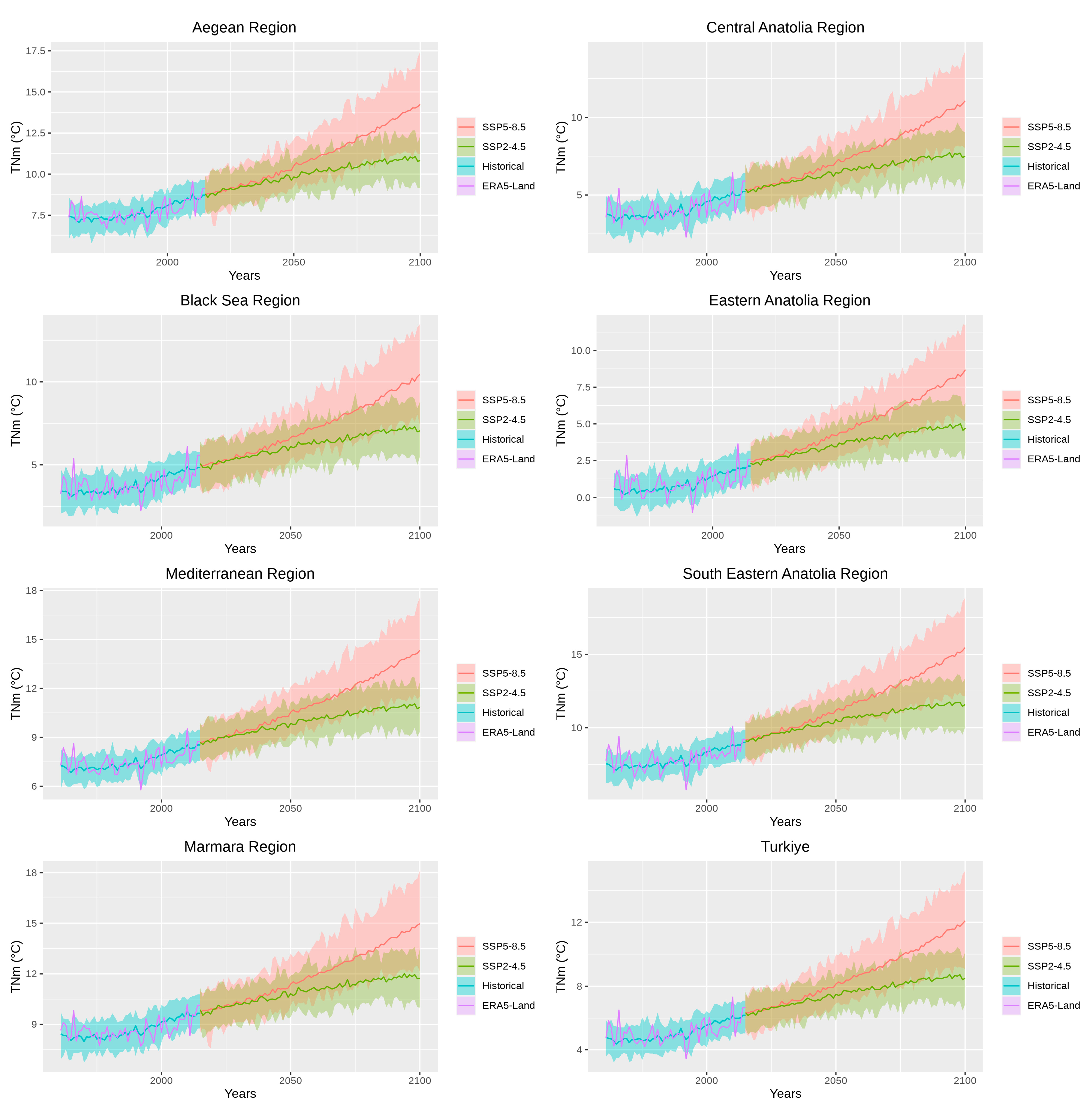
The average values of the daily minimum temperatures, TNm in Table 5, show that they are predicted to increase over time in Türkiye, especially in the late periods. Also, temporal variations in TNm in Türkiye and for the sub-regions are represented for 1961–2100 with two scenarios in Figure 13.
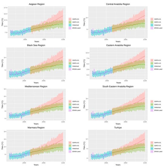
Figure 13.
Time series of TNm over historical period and 2015–2100 under the two scenarios in the seven sub-regions and across Türkiye. The top and bottom boundaries of shaded area are the 97.5th and 2.5th percentiles of the GCMs.
Considering the changes, what is striking is that the increases in this index are lower than the changes in the TNn and TNx indices. Considering the Türkiye average, the value was 5.1 °C in the historical period, reaching 8.4 °C and 10.7 °C in the SSP2-4.5 and SSP5-8.5 scenarios at the end of the century, which means 3.3 °C and 5.6 °C increases (Figure 13). However, both scenarios predicted higher increases for TNn and TNx indices. This shows that the extremes are affected more than the average when the minimum temperatures are evaluated.
Maximum Temperature Indices
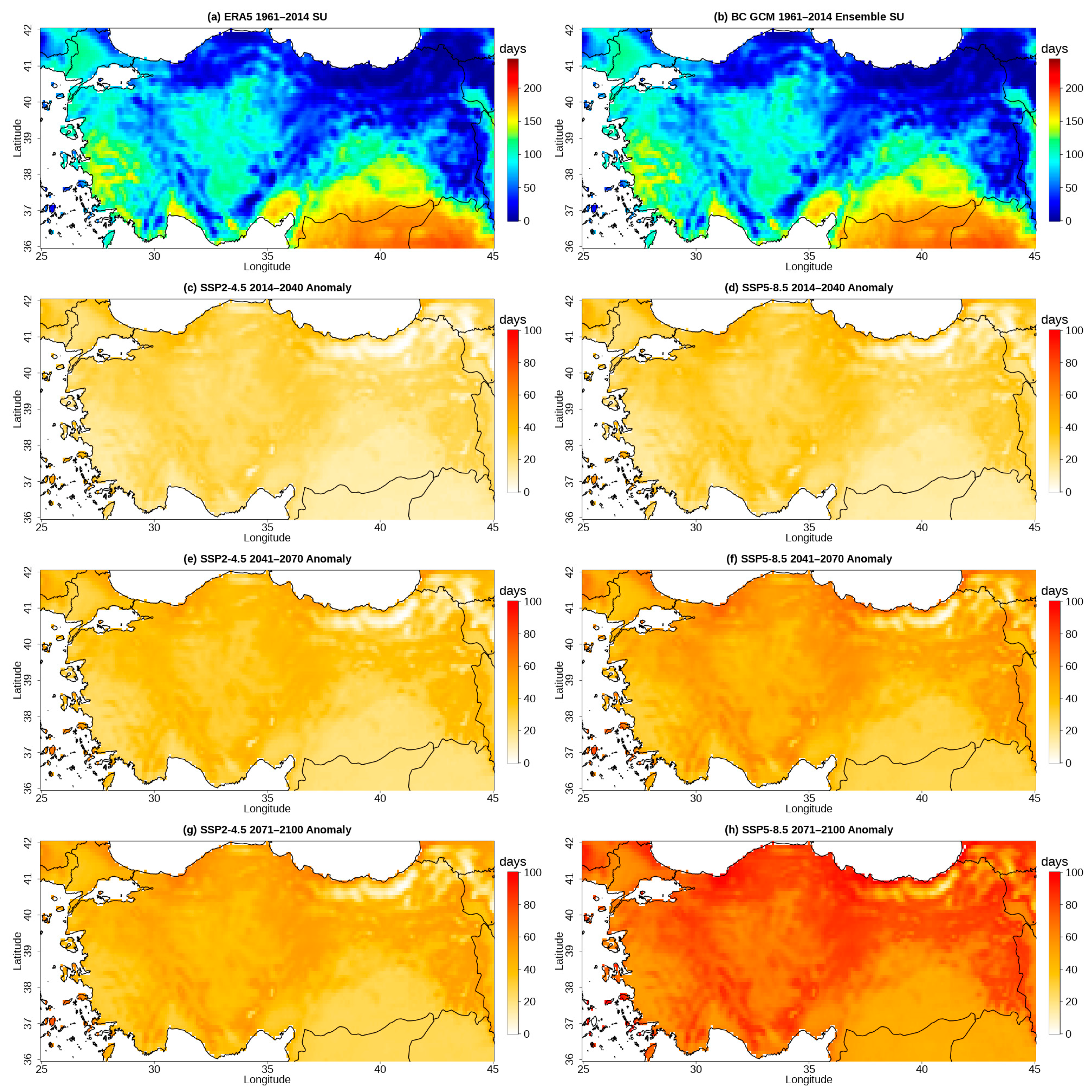
The results for six extreme maximum temperature indices are given for different time periods and two projection scenarios in Table 6 (ID, SU, WSDI, TXx, TXn, TXm) and the spatial distribution of SU is represented for 1961–2014 and 2015–2100 periods under the two scenarios in Figure 14.

Table 6.
Values of the six ETIs in the seven sub-regions and Türkiye under the two scenarios (SSP2-4.5 and SSP5-8.5) for historical and three future periods (15–40, 41–70, 71–100).
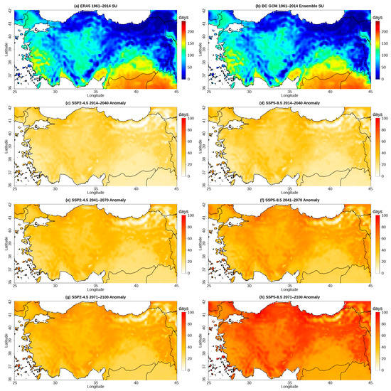
Figure 14.
Spatial distributions of the SU index during historical period (a,b) and differences from the historical period for 2015–2040 (c,d), 2041–2070 (e,f), 2071–2100 (g,h) under the SSP2-4.5 and SSP5-8.5.
The ID index in Table 6 shows the number of days where the maximum temperature is below 0 °C in a year. In the historical period, the following values can be seen: Aegean, 5.8 days; Central Anatolia, 27.0 days; Black Sea, 35.4 days; Eastern Anatolia, 64.9 days; Mediterranean, 12.5 days; Southeastern Anatolia, 13.7 days; Marmara, 5.2 days; and Türkiye, 27.7 days (Table 6). Overall, the data show a decrease in the number of icy days in each region in the future time periods compared to the historical period. This decrease is more pronounced in the mid- and late century. The most serious decrease was seen at the end of the century under the SSP5-8.5 scenario in Eastern Anatolia, where the ID dropped from 64.9 to 18.6. In the Aegean and Marmara regions, where the ID was already low during the historical period, values were almost reduced to 0 days.
When the SU index values, which show the number of days with the maximum temperature above 25 °C, are considered, the highest values were observed in Southeastern Anatolia (131.8) and the lowest values were in the Black Sea (31.6 days) and Eastern Anatolia (46.8 days) regions in the historical period (Table 6). Considering the difference between the highest values and the lowest values, it should be noted that there is significant variation between regions. When different SSP scenarios are compared, it can be seen that SU values increase over time in all regions and the biggest increase is observed at the end of the century under the SSP5-8.5 scenario (Figure 14). When this scenario is examined, it is observed that the regional changes are close to each other and there is an average 70-day increase in all regions. As a result of this increase, it is predicted that at the end of the century, more than half of the year in Southeastern Anatolia can be classified as SU.
Considering the WSDI values in different regions of Türkiye, the Aegean, Central Anatolian regions and Türkiye averages have similar WSDI values ranging from 14.2 days to 14.6 days during the historical period (Table 6). While the lowest value is seen in the Black Sea regions with 10.6 days, the WSDI value reaches 19.0 days in the Southeastern Anatolia region. In the GCM SSP2-4.5 and SSP5-8.5 scenarios, WSDI values for different regions increased in the future periods as the time range progressed from 2015–2040 to 2041–2070 and 2071–2100, showing strong increases by the end of the century, especially in the SSP5-8.5 scenario. When the increase rate is taken into account, the Black Sea and Marmara regions emerge while the Southeastern Anatolia, Eastern Anatolia, Mediterranean, and Aegean regions stand out in terms of the amount of increase by the end of the century. Compared to the observation period, it is seen that Türkiye’s average has increased above 109 days in the SSP2-4.5 scenario and above 195 days in the SSP5-8.5, especially in the distant future, and this causes an expectation of an increase in both the periods of drought and the frequency of these periods (Table 6). In general, the SSP5-8.5 scenario indicates more severe water stress than the SSP2-4.5 scenario, especially in the future.
The TXx in Table 6. represents the yearly maximum of daily maximum temperatures. When the changes in the TXx values for various regions of Türkiye are examined, in the historical period, results of the Southeastern Anatolia region are the highest among all regions with a value of 38.8 °C, while the lowest values are observed in the Black Sea and Eastern Anatolia regions with 30.4 °C and 30.5 °C, respectively. It is notable that the temperatures attained at the end of the century in the SSP2-4.5 scenario were reached at the halfway point of the SSP5-8.5 scenario. In Türkiye’s average, which was 33.4 °C in the historical period, increases of 4.3 °C and 7.5 °C degrees were projected for the SSP2-4.5 and SSP5-8.5 scenarios by the end of the century.
The TXn index in Table 6 shows the minimum value of the maximum daily temperatures during the year. It is seen that the TXn index in different regions varies from −1.2 °C to −10.3 °C during the historical period. Although it is observed that the TXn index increases under all scenarios, in all regions, and in all time periods, the highest increase is observed at the end of the century under the SSP5-8.5 scenario. According to this scenario, while seven regions were below 0 degrees in the past, this number decreases to 3 at the end of the century. The Türkiye average, which was −5.6 °C during the observation period, rises to −2.2 °C and 0 °C levels, respectively, according to the SSP2-4.5 and SSP5-8.5 scenarios by the end of the century.
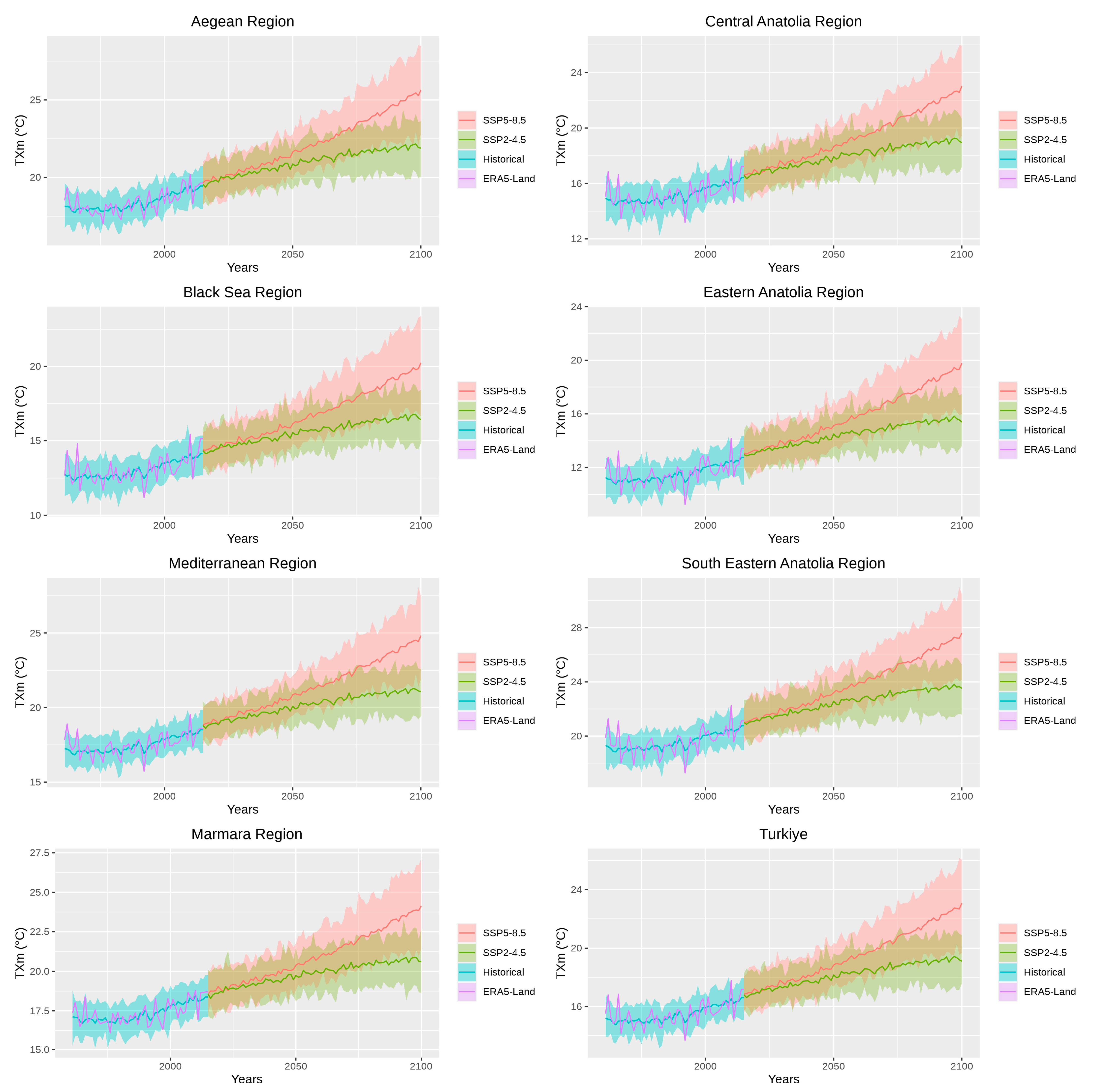
When we look at the last index (TXm) in Table 6, which shows the annual average of maximum temperatures, we can see that it is expected to increase over time in all regions. Also, temporal variations in TXm in Türkiye and for the sub-regions are represented for 1961–2100 with two scenarios in Figure 15.
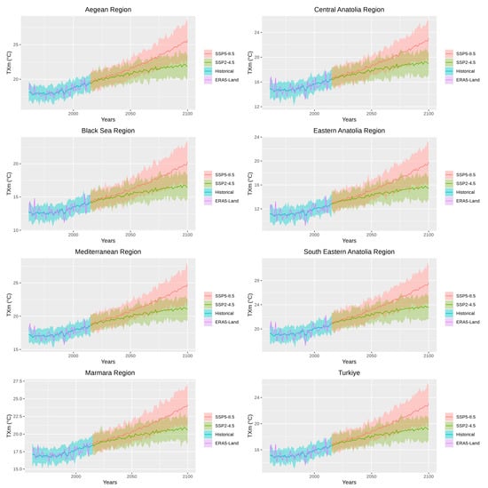
Figure 15.
Time series of TXm over historical period and 2015–2100 under the two scenarios in the seven sub-regions and across Türkiye. The top and bottom boundaries of shaded area are the 97.5th and 2.5th percentiles of the GCMs.
The rate of increase and the specific value of the maximum temperature varies between regions and time periods. For example, TXm values of the Eastern Anatolia Region are expected to experience the greatest increase (6.63 °C), while the Marmara and Black Sea regions are expected to experience the smallest increases (5.51 °C and 5.78 °C) in this index. In addition, the differences between the SSP2-4.5 and SSP5-8.5 scenarios show how different scenarios can affect future temperatures. Overall, the SSP5-8.5 scenario, which represents a future with higher levels of economic growth, technology development, and resource use, is expected to result in higher temperatures compared to the SSP2-4.5 scenario. When Turkiye’s averages are evaluated, the value that was 15.5 in the historical period is expected to increase by 3.5 °C and 5.1 °C for SSP2-4.5 and SSP5-8.5 scenarios at the end of the century (Figure 15). This shows that the TXn and TXm indices can move in parallel, while the TXx extremes may be more affected by the changes in TXm.
4. Discussion
Bagcaci et al. [29] examined the performances of CMIP5 vs. CMIP6 models in Türkiye for precipitation and temperature in detail and produced performance rankings for both variables of the examined models. In that study, ERA5 reanalysis data was used as a reference and it was concluded that CMIP6 models were more successful than CMIP5 models for both variables. The model performance ranking created in this study and the ranking created by Bagcaci et al. [29] differs on both the time scale, the compared values (yearly indices vs. monthly means), and performance metrics. Although it can be expected that there will be serious differences in the rankings given these differences, the results are similar especially for top-performing models. When the common global climate models used in only two studies are evaluated, it is revealed that 8 of the 10 most successful models for the precipitation variable are common in both studies. When the top 10 models with the best temperature performance in the two studies were compared, it was seen that seven of them were common. These results show that models that are successful in capturing monthly seasonality are also successful in annual indices. As Baghel et al. [9] pointed out, characterizing a model’s performance using statistics may be insufficient and dependent on a number of variables. Agel and Barlow [79] also outlined variations in the CMIP6 model’s ability to simulate different aspects of regional precipitation, seasonality, and distribution and underlined the importance of assessing circulation in association with precipitation.
The study conducted by Cannon et al. [36] investigated whether the relative changes in the GCM models in quantiles and extremes are preserved by quantile mapping methods when it comes to precipitation. Since QDM, which is the downscale method used in the estimation periods in this study, was also suggested by Cannon et al. [36], it is important to compare the results. The mentioned study used three CMIP6 global climate models (MIROC5, CanESM2, and CCSM4) over the Canadian domain and 1/12° grid size precipitation data obtained by Natural Resources Canada as reference data. In this study, when precipitation is in question, more than 40 CMIP6 climate models are used for the GCM historical period, while ERA5-Land precipitation data with 0.1° grid size is used as reference data. There are also differences between the periods studied. However, the biggest difference is that this study is a downscaling study, while Cannon et al. [36] focus on bias correction. In the case of bias correction, the three climate models and reference data are regridded into 1.4° grids so that they have the same size. In this application, all small observation grids falling into a GCM grid become the same size as the GCM, thus reducing the possible GCM observation differences. In downscaling, which is the basis of this study, all observation grids are directly matched with the large GCM grids they fall into without a regridding process. Because of this, the variations that may occur in reference grids that are located at two different ends of a GCM grid are accepted as they are.
When the K-S test results are compared with Cannon et al. [36], it is seen that the successes of all three raw GCMs used by Cannon et al. [36] are higher than those in this study. As mentioned, we think that the main reason for this difference is the difference between bias correction and downscaling. When the results obtained after the quantile mapping methods are compared, it is possible to say that the results are much closer and that the methods applied in both studies made significant corrections. This demonstrates the success of the applied methods. Furthermore, Kumar et al. [66] demonstrated the skill of QM methods in downscaling precipitation and found promising results. Enayati et al. [80] also indicated the potential of the QM methods when coping with precipitation and temperature; however, they also pointed out the impact of topographic features of the studied region besides transformation functions and parameter sets. This could be one of the reasons why QM methods exhibit regional differences in precipitation and temperature results in Türkiye, which has a comparatively complex and diverse topography.
Different studies, considering the Mediterranean region and Türkiye, investigated the effects of climate change on temperature and precipitation in the past. Barcikowska et al. [81] revealed that simulated climate changes suggest pronounced warming and drying over most of the Mediterranean region. Todaro et al. [45] also confirmed the progressive increase in temperature over the Mediterranean region, which is also supported by the findings of this study. Turkeş et al. [47] demonstrated a strong decrease in precipitation for almost all parts of the Türkiye and increasing intense drought conditions based on the projections of Regional Climate Model, RegCM4.4 of the International Centre for Theoretical Physics (ICTP) with MPI-ESM-MR global climate model. In this study, a decrease in the precipitation also revealed with variations in terms of the magnitude of this decrease among the regions. Nevertheless, the results of Uzuner and Dengiz’s [48] research highlight the desertification risk in Türkiye, which shows the increasing fragility of the region when taking account the drying conditions mentioned above. Furthermore, a recent study from Ozturk [49], using the HIRHAM5 regional climate model driven by CMIP5 global climate models EC-EARTH, HadGEM2-ES, and NorESM1-M, calculated the extreme indices in the entire Mediterranean basin at the end of the century (2071–2100) and compared them to the reference period (1971–2000). For this reason, it is similar to this study in terms of the study area and the variables examined. However, it should be noted that there is both a dynamic statistical downscaling and a CMIP5-CMIP6 GCM generation difference between studies.
When the results in Türkiye are compared with Ozturk [49], although there are differences between the models, it is possible to say that there is a consensus in terms of both the regional distribution and magnitude of climate change trends. When the results for the TXx index are examined, the averages of the three models used by Ozturk [49] show that this index will increase by 7–8 °C by the end of the century under the RCP 8.5 scenario in Türkiye, while the models driven by EC-EARTH and NorESM1-M show that the temperature changes will be equally distributed across Türkiye. However, the model driven by HadGEM2-ES predicted increases of about 10 °C for the Eastern Anatolia region while the rest of Türkiye increased by 8 °C. The multi-model ensemble produced in this study shows that the TXx index will increase by 7.5 °C at the end of the century under the SSP5-8.5 scenario in Türkiye, and the regional changes will be distributed almost equally. When the PRCPTOT index, which examines the total precipitation, is investigated, the most striking result is that the regions with the highest decrease are common in both studies. While the Aegean and Mediterranean regions will experience the highest precipitation decreases under the RCP 8.5 scenario according to all three of the models used by Ozturk [49], in this study, the multi-model ensemble obtained as a result of downscaling of more than 30 CMIP6 models with QDM predicted that the highest decreases will also occur in these two regions.
In addition, Ozturk et al. [82] also investigated the future changes in extreme climate indices over the Middle East and North Africa (MENA) and showed that as radiative forcing increases, the extreme temperature indices experience increasing intensity. They showed that while the Mediterranean region was anticipated to be particularly impacted, the entire region was projected to see significant increases in the daily maximum temperatures. Mistry [83] pointed out that detecting such common hotspot areas that potentially experience extreme weather conditions can be beneficial for policymakers, insurance providers, and urban planners to evaluate the exposure of regions to weather-related disasters. Thus, it is a significant result that should be taken into account that this study and different studies on Türkiye, and Mediterranean in which climate models of different generations are used with different downscaling methods [49,82], point to danger in the similar regions. Nonetheless, indices alone cannot convey the complete picture, and they may require examination alongside other indicators such as the use of variables and indicators, particularly for the implications of future projections of change, as outlined by Alexander et al. [84]. Increasing SDII, decreasing total precipitation, and displayed dry day conditions and their spatio-temporal variations displayed in this study also support Alexander et al. [84].
5. Conclusions and Remarks
This study aimed to investigate the spatiotemporal variations in temperature and precipitation extremes in Türkiye between 1961 and 2100, using the recently released CMIP6 GCM data. Model biases were corrected based on the European Centre for Medium-Range Weather Forecasts Reanalysis 5-Land (ERA5-Land) dataset whose accuracy in representing temperature and precipitation has already been evaluated and confirmed as sufficient. Bias-corrected high-resolution datasets were then used to produce the selected ET-SCI indices of the two future scenarios of SSP2-4.5 and SSP5-8.5. The downscaling of temperature and precipitation data from over 40 GCMs showed satisfactory performance in reproducing the 12 EPIs and 12 ETIs during the historical period. The primary findings of this study include:
- In general, all three bias correction algorithms are robust and capable of correcting large systematic biases that are present in the GCM representations of the ET-SCI indices over the historical simulation period.
- Intermodel agreement is better for temperature simulations compared to precipitation simulations.
- The temporal variations of the 12 EPIs and 12 ETIs from 2015 to 2100 consistently suggest drier conditions, yet more frequent and severe precipitation extremes and warming temperature extremes in Türkiye, under the two scenarios. The changes in the 12 EPIs and 12 ETIs were more significant for SSP5-8.5.
- Considering the dry day conditions, the Black Sea and Marmara regions emerge with greater dry periods compared to the Türkiye average, which means greater sensitivity to climate change than the other regions. In general, the SSP5-8.5 scenario indicates more severe water stress than the SSP2-4.5 scenario, especially in the future.
- Precipitation extremes indicate a decrease in the frequency of heavy rains but an increase in very heavy rains and an increasing contribution of very heavy rain days to the total precipitation. The increasing SDII and decreasing total precipitation also support these findings.
- Temperature extremes such as the coldest, warmest, and mean daily maximum temperature are expected to increase in all regions across Türkiye, indicating warming conditions. Additionally, the coldest daily maximums exhibit higher sensitivity to climate change in the Aegean, Southeastern Anatolia, Marmara, and Mediterranean regions of Türkiye, while the mean daily maximum temperature showed greater sensitivity in the Black Sea, Central Anatolia, and Eastern Anatolia regions.
The results of the analyses conducted with the most current CMIP6 climate models in this study are consistent with those of other studies of the Mediterranean climate in the literature. For sustainable developments in hydrological systems, forestry, and agriculture, these results are of great significance. It should be noted that understanding climate change is essential for both adapting to the changes and avoiding their negative effects when carrying out sustainable sectoral projects.
Author Contributions
Conceptualization, B.G., S.O. and I.Y.; data curation, B.G.; formal analysis, B.G.; investigation, B.G., S.O. and I.Y.; methodology, B.G., S.O. and I.Y.; software, B.G.; supervision, I.Y. and M.T.Y.; visualization, B.G. and S.O.; writing—original draft, B.G. and S.O.; writing—review and editing, I.Y. and M.T.Y. All authors have read and agreed to the published version of the manuscript.
Funding
This research received no external funding.
Institutional Review Board Statement
Not applicable.
Informed Consent Statement
Not applicable.
Data Availability Statement
CMIP6 data supporting this study’s findings are freely available from ESGF (https://esgf-node.llnl.gov/search/cmip6/, accessed on 14 March 2023).
Acknowledgments
This work is conducted as a part of the “High-Resolution Assessment of the Climate Change Impacts over Extreme Precipitation in Turkey using State of the Art Climate (CMIP6) Models” project supported by The Scientific and Technological Research Council of Türkiye (Grant No: 122Y259).
Conflicts of Interest
The author declares no conflict of interest.
References
- Brás, T.A.; Seixas, J.; Carvalhais, N.; Jägermeyr, J. Severity of drought and heatwave crop losses tripled over the last five decades in Europe. Environ. Res. Lett. 2021, 16, 65012. [Google Scholar] [CrossRef]
- Carnicer, J.; Alegria, A.; Giannakopoulos, C.; Di Giuseppe, F.; Karali, A.; Koutsias, N.; Lionello, P.; Parrington, M.; Vitolo, C. Global warming is shifting the relationships between fire weather and realized fire-induced CO2 emissions in Europe. Sci. Rep. 2022, 12, 10365. [Google Scholar] [CrossRef]
- AghaKouchak, A.; Cheng, L.; Mazdiyasni, O.; Farahmand, A. Global warming and changes in risk of concurrent climate extremes: Insights from the 2014 California drought. Geophys. Res. Lett. 2014, 41, 8847–8852. [Google Scholar] [CrossRef]
- Roshani, A.; Parak, F.; Esmaili, H. Trend analysis of climate change compound indices in Iran. J. Water Clim. Chang. 2020, 12, 801–816. [Google Scholar] [CrossRef]
- Kim, Y.H.; Min, S.K.; Zhang, X.; Sillmann, J.; Sandstad, M. Evaluation of the CMIP6 multi-model ensemble for climate extreme indices. Weather. Clim. Extrem. 2020, 29, 100269. [Google Scholar] [CrossRef]
- Iyakaremye, V.; Zeng, G.; Zhang, G. Changes in extreme temperature events over Africa under 1.5 and 2.0 °C global warming scenarios. Int. J. Clim. 2021, 41, 1506–1524. [Google Scholar] [CrossRef]
- IPCC. IPCC Climate Change 2021: The Physical Science Basis: Working Group I Contribution to the Sixth Assessment Report of the Intergovernmental Panel on Climate Change; Cambridge University Press: Cambridge, UK, 2021. [Google Scholar]
- Chiang, F.; Mazdiyasni, O.; AghaKouchak, A. Evidence of anthropogenic impacts on global drought frequency, duration, and intensity. Nat. Commun. 2021, 12, 2754. [Google Scholar] [CrossRef] [PubMed]
- Baghel, T.; Babel, M.S.; Shrestha, S.; Salin, K.R.; Virdis, S.G.; Shinde, V. A generalized methodology for ranking climate models based on climate indices for sector-specific studies: An application to the Mekong sub-basin. Sci. Total Environ. 2022, 829, 154551. [Google Scholar] [CrossRef] [PubMed]
- Guan, J.; Yao, J.; Li, M.; Li, D.; Zheng, J. Historical changes and projected trends of extreme climate events in Xinjiang, China. Clim. Dyn. 2022, 59, 1753–1774. [Google Scholar] [CrossRef]
- CRED. Disasters in Numbers 2021; Centre for Research on the Epidemiology of Disasters (CRED): Brussels, Belgium, 2021. [Google Scholar]
- Myhre, G.; Alterskjær, K.; Stjern, C.W.; Hodnebrog, Ø.; Marelle, L.; Samset, B.H.; Stohl, A. Frequency of extreme precipitation increases extensively with event rareness under global warming. Sci. Rep. 2019, 9, 16063. [Google Scholar] [CrossRef]
- Donat, M.G.; Lowry, A.L.; Alexander, L.V.; O’Gorman, P.A.; Maher, N. More extreme precipitation in the worldâ €TM s dry and wet regions. Nat. Clim. Chang. 2016, 6, 508–513. [Google Scholar] [CrossRef]
- Papalexiou, S.M.; Montanari, A. Global and regional increase of precipitation extremes under global warming. Water Resour. Res. 2019, 55, 4901–4914. [Google Scholar] [CrossRef]
- Donat, M.G.; Sillmann, J.; Wild, S.; Alexander, L.V.; Lippmann, T.; Zwiers, F.W. Consistency of Temperature and Precipitation Extremes across Various Global Gridded In Situ and Reanalysis Datasets. J. Clim. 2014, 27, 5019–5035. [Google Scholar] [CrossRef]
- Yao, J.; Chen, Y.; Chen, J.; Zhao, Y.; Tuoliewubieke, D.; Li, J.; Yang, L.; Mao, W. Intensification of extreme precipitation in arid Central Asia. J. Hydrol. 2020, 598, 125760. [Google Scholar] [CrossRef]
- Martinez-Villalobos, C.; Neelin, J.D. Regionally high risk increase for precipitation extreme events under global warming. Sci. Rep. 2023, 13, 5579. [Google Scholar] [CrossRef] [PubMed]
- Schleussner, C.F.; Lissner, T.K.; Fischer, E.M.; Wohland, J.; Perrette, M.; Golly, A.; Rogelj, J.; Childers, K.; Schewe, J.; Frieler, K.; et al. Differential climate impacts for policy-relevant limits to global warming: The case of 1.5 °C and 2 °C. Earth Syst. Dyn. 2016, 7, 327–351. [Google Scholar] [CrossRef]
- Kouman, K.D.; Kabo-bah, A.T.; Kouadio, B.H.; Akpoti, K. Spatio-Temporal Trends of Precipitation and Temperature Extremes across the North-East Region of Côte d’Ivoire over the Period 1981–2020. Climate 2022, 10, 74. [Google Scholar] [CrossRef]
- Moazenzadeh, R.; Mohammadi, B.; Shamshirband, S.; Chau, K. Coupling a firefly algorithm with support vector regression to predict evaporation in northern Iran. Eng. Appl. Comput. Fluid Mech. 2018, 12, 584–597. [Google Scholar] [CrossRef]
- Wang, L.; Li, Y.; Li, M.; Li, L.; Liu, F.; Liu, D.L.; Pulatov, B. Projection of precipitation extremes in China’s mainland based on the statistical downscaled data from 27 GCMs in CMIP6. Atmos. Res. 2022, 280, 106462. [Google Scholar] [CrossRef]
- Wudineh, F.A.; Moges, S.; Kidanewold, B.B. Detecting Hydrological Variability in Precipitation Extremes: Application of Reanalysis Climate Product in Data-Scarce Wabi Shebele Basin of Ethiopia. J. Hydrol. Eng. 2022, 27, 5021035. [Google Scholar] [CrossRef]
- McGree, S.; Herold, N.; Alexander, L.; Schreider, S.; Kuleshov, Y.; Ene, E.; Finaulahi, S.; Inape, K.; Mackenzie, B.; Malala, H.; et al. Recent Changes in Mean and Extreme Temperature and Precipitation in the Western Pacific Islands. J. Clim. 2019, 32, 4919–4941. [Google Scholar] [CrossRef]
- Alexander, L.; Herold, N. ClimPACT2: Indices and Software. A Document Prepared on Behalf of the Commission for Climatology (CCl) Expert Team on Sector-Specific Climate Indices (ET-SCI); University of South New Wales: Sydney, Australia, 2016. [Google Scholar]
- Yosef, Y.; Aguilar, E.; Alpert, P. Changes in extreme temperature and precipitation indices: Using an innovative daily homogenized database in Israel. Int. J. Climatol. 2019, 39, 5022–5045. [Google Scholar] [CrossRef]
- Chapagain, D.; Dhaubanjar, S.; Bharati, L. Unpacking future climate extremes and their sectoral implications in western Nepal. Clim. Chang. 2021, 168, 8. [Google Scholar] [CrossRef]
- Eyring, V.; Bony, S.; Meehl, G.A.; Senior, C.A.; Stevens, B.; Stouffer, R.J.; Taylor, K.E. Overview of the Coupled Model Intercomparison Project Phase 6 (CMIP6) experimental design and organization. Geosci. Model Dev. 2016, 9, 1937–1958. [Google Scholar] [CrossRef]
- Srivastava, A.; Grotjahn, R.; Ullrich, P.A. Evaluation of historical CMIP6 model simulations of extreme precipitation over contiguous US regions. Weather. Clim. Extrem. 2020, 29, 100268. [Google Scholar] [CrossRef]
- Bağçaci, S.Ç.; Yucel, I.; Duzenli, E.; Yilmaz, M.T. Intercomparison of the expected change in the temperature and the precipitation retrieved from CMIP6 and CMIP5 climate projections: A Mediterranean hot spot case, Turkiye. Atmos. Res. 2021, 256, 105576. [Google Scholar] [CrossRef]
- Davy, R.; Outten, S. The Arctic Surface Climate in CMIP6: Status and Developments since CMIP5. J. Clim. 2020, 33, 8047–8068. [Google Scholar] [CrossRef]
- Bayar, A.S.; Yılmaz, M.T.; Yücel, İ.; Dirmeyer, P. CMIP6 Earth system models project greater acceleration of climate zone change due to stronger warming rates. Earth’s Future 2023, 11, e2022EF002972. [Google Scholar] [CrossRef]
- Otto-Bliesner, B.L.; Brady, E.C.; Zhao, A.; Brierley, C.M.; Axford, Y.; Capron, E.; Govin, A.; Hoffman, J.S.; Isaacs, E.; Kageyama, M.; et al. Large-scale features of Last Interglacial climate: Results from evaluating the lig127k simulations for the Coupled Model Intercomparison Project (CMIP6)–Paleoclimate Modeling Intercomparison Project (PMIP4). Clim. Past 2021, 17, 63–94. [Google Scholar] [CrossRef]
- Emanuel, K. Response of Global Tropical Cyclone Activity to Increasing CO2: Results from Downscaling CMIP6 Models. J. Clim. 2021, 34, 57–70. [Google Scholar] [CrossRef]
- Dosio, A.; Jury, M.W.; Almazroui, M.; Ashfaq, M.; Diallo, I.; Engelbrecht, F.A.; Klutse, N.A.B.; Lennard, C.; Pinto, I.; Sylla, M.B.; et al. Projected future daily characteristics of African precipitation based on global (CMIP5, CMIP6) and regional (CORDEX, CORDEX-CORE) climate models. Clim. Dyn. 2021, 57, 3135–3158. [Google Scholar] [CrossRef]
- Meresa, H.; Tischbein, B.; Mekonnen, T. Climate change impact on extreme precipitation and peak flood magnitude and frequency: Observations from CMIP6 and hydrological models. Nat. Hazards 2022, 111, 2649–2679. [Google Scholar] [CrossRef]
- Cannon, A.J.; Sobie, S.R.; Murdock, T.Q. Bias Correction of GCM Precipitation by Quantile Mapping: How Well Do Methods Preserve Changes in Quantiles and Extremes? J. Clim. 2015, 28, 6938–6959. [Google Scholar] [CrossRef]
- Guo, Q.; Chen, J.; Zhang, X.; Shen, M.; Chen, H.; Guo, S. A new two-stage multivariate quantile mapping method for bias correcting climate model outputs. Clim. Dyn. 2019, 53, 3603–3623. [Google Scholar] [CrossRef]
- Tong, Y.; Gao, X.; Han, Z.; Xu, Y.; Xu, Y.; Giorgi, F. Bias correction of temperature and precipitation over China for RCM simulations using the QM and QDM methods. Clim. Dyn. 2021, 57, 1425–1443. [Google Scholar] [CrossRef]
- Hersbach, H.; Bell, B.; Berrisford, P.; Hirahara, S.; Horanyi, A.; Muñoz-Sabater, J.; Nicolas, J.; Peubey, C.; Radu, R.; Schepers, D.; et al. The ERA5 global reanalysis. Q. J. R. Meteorol. Soc. 2020, 146, 1999–2049. [Google Scholar] [CrossRef]
- Muñoz-Sabater, J.; Dutra, E.; Agustí-Panareda, A.; Albergel, C.; Arduini, G.; Balsamo, G.; Boussetta, S.; Choulga, M.; Harrigan, S.; Hersbach, H.; et al. ERA5-Land: A state-of-the-art global reanalysis dataset for land applications. Earth Syst. Sci. Data 2021, 13, 4349–4383. [Google Scholar] [CrossRef]
- Brogli, R.; Sørland, S.L.; Kröner, N.; Schär, C. Causes of future Mediterranean precipitation decline depend on the season. In Proceedings of the EGU General Assembly 2020, Online, 4–8 May 2020. EGU2020-4638. [Google Scholar] [CrossRef]
- Tramblay, Y.; Koutroulis, A.G.; Samaniego, L.; Vicente-Serrano, S.M.; Volaire, F.; Boone, A.; Page, M.L.; Llasat, M.D.; Albergel, C.; Burak, S.; et al. Challenges for drought assessment in the Mediterranean region under future climate scenarios. Earth-Sci. Rev. 2020, 210, 103348. [Google Scholar] [CrossRef]
- Tuel, A.; Eltahir, E.A.B. Why Is the Mediterranean a Climate Change Hot Spot? J. Clim. 2020, 33, 5829–5843. [Google Scholar] [CrossRef]
- Driouech, F.; ElRhaz, K.; Moufouma-Okia, W.; Arjdal, K.; Balhane, S. Assessing Future Changes of Climate Extreme Events in the CORDEX-MENA Region Using Regional Climate Model ALADIN-Climate. Earth Syst. Environ. 2020, 4, 477–492. [Google Scholar] [CrossRef]
- Todaro, V.; D’Oria, M.; Secci, D.; Zanini, A.; Tanda, M.G. Climate Change over the Mediterranean Region: Local Temperature and Precipitation Variations at Five Pilot Sites. Water 2022, 14, 2499. [Google Scholar] [CrossRef]
- Aziz, R.; Yücel, İ. Assessing nonstationarity impacts for historical and projected extreme precipitation in Turkey. Theor. Appl. Climatol. 2021, 143, 1213–1226. [Google Scholar] [CrossRef]
- Türkeş, M.; Turp, M.T.; An, N.; Öztürk, T.; Kurnaz, M.L. Impacts of Climate Change on Precipitation Climatology and Variability in Turkey. Water Resour. Turk. 2020, 2, 467–491. [Google Scholar] [CrossRef]
- Uzuner, C.; Dengiz, O. Desertification risk assessment in Turkiye based on environmentally sensitive areas. Ecol. Indic. 2020, 114, 106295. [Google Scholar] [CrossRef]
- Öztürk, T. Projections of Future Change of Climatology and Extreme Events in the Mediterranean Basin, by the HIRHAM5. Int. J. Adv. Eng. Pure Sci. 2022, 34, 167–189. [Google Scholar] [CrossRef]
- Sen, O.L.; Unal, A.; Bozkurt, D.; Kindap, T. Temporal changes in the Euphrates and Tigris discharges and teleconnections. Environ. Res. Lett. 2011, 6, 24012. [Google Scholar] [CrossRef]
- Bozkurt, D.; Sen, O. Climate change impacts in the Euphrates-Tigris Basin based on different model and scenario simulations. J. Hydrol. 2013, 480, 149–161. [Google Scholar] [CrossRef]
- Yucel, I.; Güventürk, A.; Sen, O.L. Climate change impacts on snowmelt runoff for mountainous transboundary basins in eastern Turkiye. Int. J. Climatol. 2015, 35, 215–228. [Google Scholar] [CrossRef]
- Aziz, R.; Yucel, I.; Yozgatligil, C. Nonstationarity impacts on frequency analysis of yearly and seasonal extreme temperature in Turkiye. Atmos. Res. 2020, 238, 104875. [Google Scholar] [CrossRef]
- Sensoy, S.; Türkoğlu, N.; Akçakaya, A.; Ulupınar, Y.; Ekici, M.; Demircan, M.; Atay, H.; Tüvan, A.; Demirbaş, H. Trends in Turkey climate indices from 1960 to 2010. In Proceedings of the 6th Atmospheric Science Symposium, ITU, Istanbul, Turkey, 24–26 April 2013. [Google Scholar]
- Abbasnia, M.; Toros, H. Trend analysis of weather extremes across the coastal and non-coastal areas (case study: Turkey). J. Earth Syst. Sci. 2020, 129, 95. [Google Scholar] [CrossRef]
- Oruc, S. Performance of bias corrected monthly CMIP6 climate projections with different reference period data in Turkey. Acta Geophys. 2022, 70, 777–789. [Google Scholar] [CrossRef]
- Amjad, M.R.; Yilmaz, M.T.; Yucel, I.; Yilmaz, K.K. Performance evaluation of satellite- and model-based precipitation products over varying climate and complex topography. J. Hydrol. 2020, 584, 124707. [Google Scholar] [CrossRef]
- General Diroctorate of Meteorology (GDM). Offical Statistics/Parameter Analysis. 2023. Available online: https://www.mgm.gov.tr/FILES/iklim/yillikiklim/2022-iklim-raporu.pdf (accessed on 1 March 2023).
- Yilmaz, M. Accuracy assessment of temperature trends from ERA5 and ERA5-Land. Sci. Total Environ. 2023, 856, 159182. [Google Scholar] [CrossRef] [PubMed]
- Stouffer, R.J.; Eyring, V.; Meehl, G.A.; Bony, S.; Senior, C.A.; Stevens, B.; Taylor, K.E. CMIP5 Scientific Gaps and Recommendations for CMIP6. Bull. Am. Meteorol. Soc. 2017, 98, 95–105. [Google Scholar] [CrossRef]
- Liu, X.; Li, C.; Zhao, T.; Han, L. Future changes of global potential evapotranspiration simulated from CMIP5 to CMIP6 models. Atmos. Ocean. Sci. Lett. 2020, 13, 568–575. [Google Scholar] [CrossRef]
- Wyser, K.; Kjellström, E.; Königk, T.; Martins, H.; Doescher, R. Warmer climate projections in EC-Earth3-Veg: The role of changes in the greenhouse gas concentrations from CMIP5 to CMIP6. Environ. Res. Lett. 2020, 15, 54020. [Google Scholar] [CrossRef]
- Afshar, M.H.; Yilmaz, M.T. The Added Utility of Nonlinear Methods Compared To Linear Methods In Rescaling Soil Moisture Products. Remote Sens. Environ. 2017, 196, 224–237. [Google Scholar] [CrossRef]
- Afshar, M.H.; Yilmaz, M.T.; Crow, W.T. Impact of rescaling approaches in simple fusion of soil moisture products. Water Resour. Res. 2019, 55, 7804–7825. [Google Scholar] [CrossRef]
- Heo, J.-H.; Ahn, H.; Shin, J.-Y.; Kjeldsen, T.R.; Jeong, C. Probability Distributions for a Quantile Mapping Technique for a Bias Correction of Precipitation Data: A Case Study to Precipitation Data Under Climate Change. Water 2019, 11, 1475. [Google Scholar] [CrossRef]
- Niranjan Kumar, K.; Thota, M.S.; Ashrit, R.; Mitra, A.K.; Rajeevan, M. Quantile mapping bias correction methods to IMDAA reanalysis for calibrating NCMRWF unified model operational forecasts. Hydrol. Sci. J. 2022, 67, 870–885. [Google Scholar] [CrossRef]
- Chen, J.; Brissette, F.P.; Chaumont, D.; Braun, M. Performance and uncertainty evaluation of empirical downscaling methods in quantifying the climate change impacts on hydrology over two North American river basins. J. Hydrol. 2013, 479, 200–214. [Google Scholar] [CrossRef]
- Kim, S.; Joo, K.; Kim, H.; Shin, J.-Y.; Heo, J.-H. Regional quantile delta mapping method using regional frequency analysis for regional climate model precipitation. J. Hydrol. 2021, 596, 125685. [Google Scholar] [CrossRef]
- Wang, F.; Tian, D. On deep learning-based bias correction and downscaling of multiple climate models simulations. Clim. Dyn. 2022, 59, 3451–3468. [Google Scholar] [CrossRef]
- Bürger, G.; Murdock, T.Q.; Werner, A.T.; Sobie, S.R.; Cannon, A.J. Downscaling extremes—An intercomparison of multiple statistical methods for present climate. J. Clim. 2012, 25, 4366–4388. [Google Scholar] [CrossRef]
- Kim, J.; Ivanov, V.Y.; Fatichi, S. Climate change and uncertainty assessment over a hydroclimatic transect of Michigan. Stoch. Environ. Res. Risk Assess 2016, 30, 923–944. [Google Scholar] [CrossRef]
- Ahmed, K.; Sachindra, D.A.; Shahid, S.; Demirel, M.C.; Chung, E.S. Selection of multi-model ensemble of general circulation models for the simulation of precipitation and maximum and minimum temperature based on spatial assessment metrics. Hydrol. Earth Syst. Sci. 2019, 23, 4803–4824. [Google Scholar] [CrossRef]
- Grose, M.R.; Narsey, S.; Delage, F.; Dowdy, A.J.; Bador, M.; Boschat, G.; Chung, C.T.; Kajtar, J.B.; Rauniyar, S.P.; Freund, M.B.; et al. Insights from CMIP6 for Australia’s Future Climate. Earth’s Future 2020, 8, e2019EF001469. [Google Scholar] [CrossRef]
- Cooley, A.K.; Chang, H. Detecting change in precipitation indices using observed (1977–2016) and modeled future climate data in Portland, Oregon, USA. J. Water Clim. Chang. 2021, 12, 1135–1153. [Google Scholar] [CrossRef]
- Sillmann, J.; Kharin, V.V.; Zwiers, F.W.; Zhang, X.; Bronaugh, D. Climate extreme indices in the CMIP5 multimodel ensemble: Part 2. Future climate projections. J. Geophys. Res. 2013, 118, 2473–2493. [Google Scholar] [CrossRef]
- Guan, T.; Liu, Y.; Sun, Z.; Zhang, J.; Chen, H.; Wang, G.; Jin, J.; Bao, Z.; Qi, W. A Framework to Identify the Uncertainty and Credibility of GCMs for Projected Future Precipitation: A Case Study in the Yellow River Basin, China. Front. Environ. Sci. 2022, 10, 863575. [Google Scholar] [CrossRef]
- Sherwood, S.C.; Webb, M.J.; Annan, J.D.; Armour, K.C.; Forster, P.M.; Hargreaves, J.C.; Hegerl, G.; Klein, S.A.; Marvel, K.D.; Rohling, E.J.; et al. An Assessment of Earth’s Climate Sensitivity Using Multiple Lines of Evidence. Rev. Geophys. 2020, 58, e2019RG000678. [Google Scholar] [CrossRef] [PubMed]
- Bjordal, J.; Storelvmo, T.; Alterskjær, K.; Carlsen, T. Equilibrium climate sensitivity above 5 °C plausible due to state-dependent cloud feedback. Nat. Geosci. 2020, 13, 718–721. [Google Scholar] [CrossRef]
- Agel, L.; Barlow, M. How Well Do CMIP6 Historical Runs Match Observed Northeast, U.S. Precipitation and Extreme Precipitation–Related Circulation? J. Clim. 2020, 33, 9835–9848. [Google Scholar] [CrossRef]
- Enayati, M.; Bozorg-Haddad, O.; Bazrafshan, J.; Hejabi, S.; Chu, X. Bias correction capabilities of quantile mapping methods for rainfall and temperature variables. J. Water Clim. Chang. 2021, 12, 401–419. [Google Scholar] [CrossRef]
- Barcikowska, M.J.; Kapnick, S.B.; Krishnamurty, L.; Russo, S.; Cherchi, A.; Folland, C.K. Changes in the future summer Mediterranean climate: Contribution of teleconnections and local factors. Earth Syst. Dynam. 2020, 11, 161–181. [Google Scholar] [CrossRef]
- Ozturk, T.; Saygili-Araci, F.S.; Kurnaz, M.L. Projected Changes in Extreme Temperature and Precipitation Indices Over CORDEX-MENA Domain. Atmosphere 2021, 12, 622. [Google Scholar] [CrossRef]
- Mistry, M. A High-Resolution Global Gridded Historical Dataset of Climate Extreme Indices. Data 2019, 4, 41. [Google Scholar] [CrossRef]
- Alexander, L.V.; Fowler, H.J.; Bador, M.; Behrangi, A.; Donat, M.G.; Dunn, R.J.; Funk, C.; Goldie, J.; Lewis, E.; Rogé, M.; et al. On the use of indices to study extreme precipitation on sub-daily and daily timescales. Environ. Res. Lett. 2019, 14, 125008. [Google Scholar] [CrossRef]
Disclaimer/Publisher’s Note: The statements, opinions and data contained in all publications are solely those of the individual author(s) and contributor(s) and not of MDPI and/or the editor(s). MDPI and/or the editor(s) disclaim responsibility for any injury to people or property resulting from any ideas, methods, instructions or products referred to in the content. |
© 2023 by the authors. Licensee MDPI, Basel, Switzerland. This article is an open access article distributed under the terms and conditions of the Creative Commons Attribution (CC BY) license (https://creativecommons.org/licenses/by/4.0/).


