Abstract
Traditional container terminals usually use a horizontal yard layout, while automated container terminals usually use a vertical yard layout. The two types of yard layout perform differently in the vehicle travel routes, the handling interface points of vehicles and yard cranes, and the yard cranes travel routes. These differences result in the different indicators between the two types of yard layout, such as yard utilization, average vehicle travel routes, average yard crane travel distance, and overall terminal efficiency etc. This paper uses an analytic method to quantify these indicators of the two types of yard layout. Based on the analysis results, the terminal efficiency is approximated by a queuing network from the overall operations. In the experiment studies, we first evaluate the indicators of the two types of yard layout, respectively. Then, we change the length and width of the yard to compare the efficiency of the two types of yard layout in various yard sizes. Finally, the overall terminal efficiency is compared. Results show that the overall efficiency is significantly affected by the service rate of yard cranes. The results in this paper may provide references for terminal yard design.
1. Introduction
Automated container terminals have been constructed in recent years, such as ECT at the Port of Rotterdam in the Netherlands, the port of Singapore, the port of Hamburg in Germany, the Shanghai Yangshan port, et al. Compared with traditional container terminals, more automated equipment and technologies are used in automated container terminals to enhance the handling efficiency, minimize labor costs and reduce loading and unloading time for ships in port. Additionally, automated equipment is powered by electricity, leading to decreasing fuel consumption and the emissions during handling operations. Further, the automated container terminals differ from traditional container terminals in yard layout. The automated container terminal usually uses vertical yard layout (as shown in Figure 1a) and the traditional container terminal uses horizontal yard layout (as shown in Figure 1b). The choice of yard layout leads to different yard efficiency, and also has an impact on the vehicle routes.
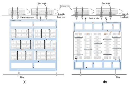
Figure 1.
Yard layout of horizontal and vertical yard layout. (a) Horizontal yard layout. (b) Vertical yard layout.
The overall operations in container terminals can be divided into three stages: the quayside operation uses the quay crane (QC) to load or unload containers between the ship and the quayside; the horizontal transportation uses AGVs or trucks to transport containers between the quayside and the yard blocks; and the yard operation uses the automated storage crane (ASC) to complete the retrieve/storage. The three stages cooperate to complete the unloading/loading ships and affect the whole terminal efficiency. In automated container terminals, automated guided vehicles (AGVs) travel between the yard blocks and the quayside, and the interface points with ASCs are in the front of yard blocks. The expected traveling distance is shorter, but the yard cranes may spend too much time retrieving containers from yard blocks, because yard cranes have to hold the container between the front point and locations. In traditional container terminals, trucks travel on the roads between the yard blocks, and the interfere points are along the yard blocks. The expected traveling distance is longer, but the yard cranes may spend too little time retrieving containers from yard blocks, because the yard cranes only carry containers to the travelling lanes of vehicles instead of the front points. The efficiency of horizontal transport and yard block will finally affect the whole efficiency.
From the above analysis, since the automated container terminal changes the yard layout, it is necessary to evaluate the overall efficiency of automated container terminals and analyze its benefit compared with traditional container terminals.
This paper uses mathematical analysis method to compare the operation efficiency of the automated container terminals and the traditional container terminals. The expected travel distance of vehicles is modeled, and then a queuing network is used to model the multiple operations in the terminal. The queuing network helps to construct the relation of multiple operations and analyze the overall efficiency of container terminals.
2. Literature Review
The ECT in the Port of Rotterdam in the Netherlands is the first automated container terminal in the world. Subsequently, the CTA terminal in Hamburg, Germany, the Shanghai Yangshan Phase IV, Qingdao Qianwan, and Xiamen Yuanhai, et al., have also built automated container terminals. The research issues in container terminals include strategic decisions and optimization of handling schedules.
The optimization of handling schedules mainly focuses on the task allocation and assignment among the automated equipment. Yu and Egbelu [1] studied the task allocation problem of the card to minimize the task time and optimize the task allocation and job position of the card. Nossack and Pesch [2] studied the task allocation problem of container trucks, analyzed the task arrangement and empty container transportation of truck companies, and established a truck task allocation model with time window to reduce truck running time. Liu et al. [3] analyzed the operational efficiency of the vertical yard layout and parallel yard layout. A simulated analysis is used to determine the optimal number of AGVs. Kemme [4] analyzed the effect of the length, height and width of a yard block on the yard efficiency, the way ARMG operates in quay yards. Additionally, he presented the operation of different numbers of ARMGs in the same block area, and analyzed the length, width and stacking height of the block area of the quay yard. The final analysis is a simulation of the operational efficiency of the terminal under different ARMG operating conditions and yard layouts. Russell D et al. [5] presented the objectives of the quay layout and analyzed the efficiency by the algorithm. Kap Hwan Kim et al. [6] applied plan layout theory to the division of container yards. They solved the problem of optimizing the allocation of non-static stacking spaces by mixing integer programming and traditional heuristics. Kevin Tierney et al. [7] explored the impact of terminal facilities and layout on container transport efficiency by using a new mixed integer programming model. Byung Kwon Lee et al. [8] have taken into account the size of the container yard and the operational capacity of the yard’s handling equipment in order to optimize the layout of the quay yard. Abu Aisha, Tareq et al. [9] built a new and efficient terminal layout by shortening the distance between the terminal and the track. The increased efficiency of container terminals is due to lower costs and faster movement of containers. Budiyanto, Muhammad Arif et al. [10] estimated the energy consumption and CO2 emissions of container terminals. They found the efficiencies of the parallel and vertical layouts are almost the same in their operation on a sustainable basis. Roy, D et al. [11] captured stochasticity through an integrated queueing network modelling approach in order to analyze the performance of container terminals with parallel stacking layouts. The conclusion is that container terminals with parallel stacking layouts perform better than terminals with vertical stacking layouts, assuming the same width of the internal transport area. Li, X.et al. [12] carried out a detailed simulation study of different types of layout designs. They built a new agent-based simulation model and this model combined side loading and end loading operations under different layout design types. Finally, they found the U-shaped automated terminal is the lowest energy and operating cost terminals.
Strategic decisions solve problems such as designing the terminal yard layout, selecting automated equipment, etc. There are two main methods to evaluate the efficiency of terminal operations: the mathematical modelling and the simulation approach [13]. Mathematical modelling mainly focuses on optimization problems, such as optimizing the operation schedules, determining the yard configuration, etc. Gharehgozli et al. [14] reviews the literature that focus on the transition of yard layout from traditional container terminals to automated container terminals. The necessary strategic and tactical layout design issues are addressed. Bassan [15] proposed some indicators for analyzing the efficiency of port operations. Chu and Huang [16] analyzed the operational efficiency of the terminals with different operating equipment and yard sizes. Vidovic and Kim [17] used queuing theory to analyze the turnaround time of trucks in the container terminal. Roy et al. [18] proposed a model for ALV loading and unloading operations in automated container terminals. They analyzed the efficiency of ALV operations using stochastic process theory. Li et al. [12] analyzes the impact of layout design on terminal performance. They use a simulation method to obtain the indicators of three types of yard layout, such as annual throughput, ship waiting time and operation efficiency of quay cranes. The above research on container terminals mainly focuses on optimization operation schedules and uses modeling and simulation methods to evaluate the container terminals. These papers provide some references for this paper. This paper compares the vertical and horizontal yard layout from the perspective of the overall operation efficiency. The aim of our paper is to compare the efficiency of the yard layout of automated container terminals with traditional container terminals. The comparisons focus on the horizontal transport efficiency, yard efficiency and overall operation efficiency. The contributions are as follows: (1) We propose a mathematical model to analyze the vehicle travel routes. The impact of yard layout of automated container terminal and traditional container terminal on horizontal transportation distance is analyzed. (2) We use a queuing network to model the operation processes of container terminals. The relationships among different processes are captured. The operation efficiency from the perspective of overall operations is compared between the two types of container terminals.
3. Modelling Approach
3.1. Problem Description
The layout of the yard blocks affects the travel routes of the vehicles between the quayside and the yard blocks, and thus affects the operating efficiency of the horizontal transportation. This paper proposes the analysis model of horizontal transport with different types of yard layout, and then model the overall operations by a queuing network.
In traditional container terminals, the yard block is parallel to the shore. There are multiple yard blocks in the horizontal direction and vertical direction. Roads are designed between the yard blocks. In the horizontal direction, the road is one-way, and the vertical direction is two-way. Trucks travel on the road, and the handling points are along the road, which are beside the bays. In Figure 2, trucks will choose the shortest path to travel from the origin to the destinated positions.
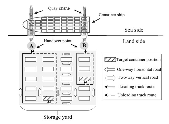
Figure 2.
Truck travel routes of traditional container terminal.
In automated container terminals, the yard layout is perpendicular to the shore, and there are multiple yard blocks in the horizontal direction. The traveling area of AGVs is between the front of quayside and the yard blocks. The AGV driving lanes are horizontal and vertical. The horizontal driving lane is one-way, and the vertical driving lane is two-way. The AGV lifts or puts down containers in front of yard blocks instead of traveling into the yard blocks. The AGV transports the container from the quayside to the yard blocks and returns to the quayside for the next task. According to the position of the quay crane and the yard block, the driving path of the AGV is shown in Figure 3.
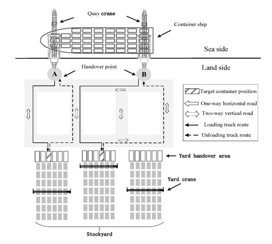
Figure 3.
AGV travel routes of automated container terminal.
3.2. Modelling the Vehicle Routes
In order to analyze the operation efficiency of the horizontal operations, this section calculates the average travel path of the vehicles under the layout of the traditional container terminal and the automated container terminals, respectively. The parameters and variables of the model are as follows:
- L: Total length of the yard;
- W: Total width of the yard;
- : The length of the AGV lane between the quayside and the yard blocks;
- X: The number of yard blocks in the horizontal direction under the automated container terminals;
- E(L): Expected travel distance of AGVs;
- E(N): Expected travel distance of trucks;
- : The distance between the yard blocks in the horizontal direction under automated container terminals;
- y: The number of yard blocks in the horizontal direction under the traditional container terminals;
- : The length of the yard blocks in the horizontal direction under the traditional container terminals;
- : The distance between the yard blocks in the horizontal direction under traditional container terminals;
- z: The number of yard blocks in the vertical direction under the traditional container terminals;
- : The distance between the yard blocks in the vertical direction under traditional container terminals;
- : Width of yard blocks;
- V: Expected travel speed of yard cranes;
- T: Time to pick up/stack one container by an ASC;
- (1)
- Yard layout of automated container terminals
In the automated container terminals, AGVs start from the quayside to the yard blocks, and then travel back to the quayside again. We assume the origin and destination at the quayside are the same. The positions of the quay cranes are discrete, and the probabilities of these positions are the same. The positions of the QCs and target yard blocks lead to the different travel routes. The horizontal transport area is divided into small areas by vertical road lanes. According to the relationship of origins and destinations of an AGV, the driving path has two situations: (1) The origin and the destination are in the same column. As shown in Figure 4, the AGVs travel from the A position at the quayside to the yard block (red line). (2) The origin and destination are not in the same column. As shown in Figure 4, the AGV travels from the B/C position at the quayside to the yard block (blue line). The expected driving distance of the AGVs in the above two cases is calculated below.
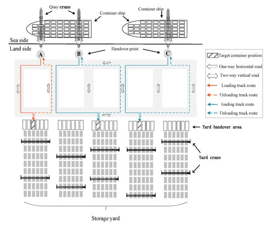
Figure 4.
Relationship of AGV routes and original/destination positions.
(1) If the origin and destination position are in the same column, the expected driving distance of the AGV is , and the probability is: . Therefore, the expected driving distance of the AGVs is:
(2) If the origin and destination position are not in the same column, there are several cases.
When the origin position is next to the destination position, the driving distance of the AGV and the probability are as follows.
When the origin position and the destination position is separated by one yard block in the horizontal direction, the driving distance of the AGV and the probability are as follows.
By analogy, when the quay crane and the target container yard block are separated by yard blocks in the horizontal direction, the driving distance of the AGV is:
Therefore, in this case, the average travel distance of the AGV is:
From case 1 and 2, the average driving distance of the AGV in automated container terminals is:
- (2)
- Yard layout of traditional container terminals
In the parallel yard layout, the positions of the horizontal yard blocks are discrete, and the probabilities of these positions are the same. The truck travel distance is affected by the position of quay crane and the target container position at the yard blocks. The positional relationship between the quay crane and the target container position at the yard blocks is mainly divided into two situations: (1) The quay crane and the target container position at the yard blocks are in the same column. For example, as shown in Figure 5, the trucks travel from the A position at the quayside to the yard block (red line). Since the road is designed to drive in one direction in the horizontal direction, the empty truck will continue to move back to the vertical road and return to point A to continue the next task. (2) The quay crane and the target container area are not in the same row. For example, the truck will start from point C to target yard block. The travel routes are shown in the blue line.
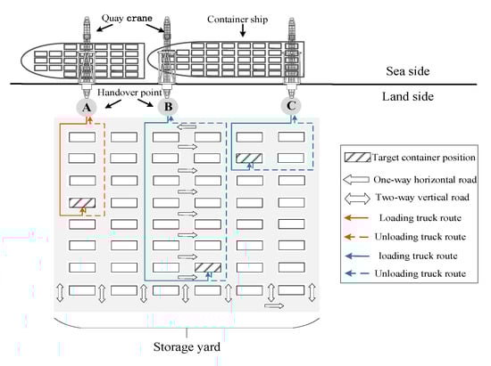
Figure 5.
Relationship of truck routes and original/destination positions.
Assuming that the road in the horizontal direction is a one-way road, first, we calculate the travel distance of trucks in each situation and the probability of each situation and then we can obtain the average truck travelling distance. Assuming that the number of yard blocks in the horizontal direction is y and the number of blocks in the vertical direction is z, the block in the first row on the far left is labeled by . By analogy, the block in the first row on the far right is . The block in the last row on the left is , and the block in the last row on the far right is . The probability that a truck travels from the quay crane position to any yard block is equal to .
When the positional relationship between the quay crane and the target yard block is the first case (the quay crane and the target yard block are in the same row), the travel distance to the yard block in the first row is:
The travel distance to the yard block in the second row is:
The travel distance to the yard block in the third row is:
By analogy, the travel distance to the yard block in the z-th row is:
There are y cases that the position of the quay crane and the target yard block is in the same column. Then, the average travel distance of the truck is:
If the quay crane and the target yard block are not in the same row, the average travel distance of the truck can be calculated according to the positional relationship between the position of the quay crane and the target yard block. When the row difference between the quay crane and the target yard block in the horizontal direction is 0, the travel distance to the block in the first row is:
The travel distance to the block in the second row is:
The travel distance to the block in the third row is:
By analogy, the travel distance from to the block in the row z is:
There are 2(y − 1) cases that the position difference between the crane and the target container area in the horizontal direction is 0, and the average travel distance of the truck is:
when the row difference between the quay crane and the target yard block in the horizontal direction is 1, the travel distance to the block in the first row is:
The travel distance to the block in the second row is:
The travel distance to the block in the third row is:
By analogy, the travel distance to the block in the z-th row is:
when the position difference between the crane and the target container area in the horizontal direction is 1, there are 2(y − 2) cases. At this time, the average travel distance of the truck is:
When the row difference between the quay crane and the target yard block in the horizontal direction is 2, the travel distance to the block in the first row is:
The travel distance to the block in the second row is:
The travel distance to the block in the third row is:
By analogy, the travel distance to the block in the z-th row is:
There are 2(y − 3) cases when the position difference between the crane and the target container area in the horizontal direction is 2. At this time, the average travel distance of the truck is:
By analogy, when the row difference between the quay crane and the target yard block in the horizontal direction is y − 2, the travel distance to the block in the first row is:
The travel distance to the block in the second row is:
The travel distance to the block in the third row is:
By analogy, the travel distance to the block in the z-th row is:
There are 2 cases when the position difference between the crane and the target container area in the horizontal direction is y − 2. At this time, the average travel distance of the truck is:
Therefore, the average travel distance of the truck in the second case is:
The probabilitis for trucks to travel from the quay crane to any yard block are equal. Then, the average traveling distance of trucks in the horizontal layout in the traditional container terminal is:
3.3. Modelling the Overall Terminal Operations
Vehicles are responsible for container transport in the terminal which travel between the quayside and yard blocks. Therefore, from the perspective of vehicle operation, the queuing process of vehicles at the quayside, on the road and at the yard blocks consist of a closed queuing network. However, the service efficiency of vehicles in the automated container terminal and traditional container terminal is not the same. Therefore, we first use a queuing network to model the operations in the terminal, and then calculate the efficiency and equipment utilization of the system. The variables of the queuing network model are as follows:
- : The number of vehicles;
- : The average traveling speed of vehicles;
- : Total width of the yard;
- : Picking up and dropping down time;
- : Travelling speed of yard cranes;
- : Loading or unloading rates at the quayside if there are vehicles;
- Loading or unloading rates at the yard blocks if there are vehicles;
- The average sojourn time of vehicles at the quayside;
- The average sojourn time of vehicles between the quayside and yard blocks;
- The average sojourn time of vehicles at the yard blocks;
- The number of quay cranes;
- The number of yard blocks;
- The probability that there are vehicles at the quayside;
- The probability that there are vehicles at the yard blocks;
- Turn-around time of vehicles in the terminal;
- : The width of a container;
- : The length of a container;
- : The distance between containers in a yard block;
We choose the turnaround time of vehicles in the terminal as the efficiency indicator, then:
- (1)
- At the quayside
The quayside operation is responsible for loading/unloading vehicles. The vehicles will directly drive the loading/unloading area if there are idle quay crane upon its arrival at the quayside. Otherwise, the vehicles will wait until there are available quay cranes. The quay cranes load or unload containers to or from the vehicles. There are two cases for the service time of quay cranes:
If there are no vehicles waiting at the quayside (), the quay crane will hold a container waiting for the vehicle. Then, the loading time for vehicles is the drop time:
If there are vehicles waiting at the quayside, the loading time equals the time from the departure time of the previous vehicle to the departure time of this vehicle. It is also the time that the trolley of the quay crane starts from the landside to the landside (a cycle). Let be the time that a trolley moves from the landside to the shipside. is the grasping time of the trolley. If there are vehicles at the quayside, the loading time of vehicles is:
In this paper, MVA (mean value analysis) method is used to calculate the average sojourn time of vehicles. is the average queueing length of vehicles if the total number of vehicles is L, then:
The probability that there are vehicles is:
- (2)
- Horizontal transport
The horizontal transportation time is affected by the yard layout. Assume that the vehicles travel at a constant speed. The avoidance during the travel time is ignored. Then, the transportation time equals to value that the transportation distance divids the speed.
- (3)
- Yard operation
(1) Automated container terminals
In the automated terminal, with the perpendicular yard layout, the handover points are at the end of each yard block. Therefore, the yard crane needs to return to the handover points to pick up the next container after completing one container.
Assuming that there are n bays of containers in one yard block, the operation time of the yard crane equals to the value that the moving distance divids by the speed. When there are AGVs waiting at the yard, the loading time of the yard crane is the time when the previous AGV departs to the time when this AGV departs. It is also the time that the yard crane returns to the initial position from the dropping position. When the dropping position is in the first bay, the moving distance of the yard crane is:
when the dropping position is in the second bay, the moving distance of the yard crane is:
when the dropping position is in the third bay, the moving distance of the yard crane is:
when the dropping position is in the n-th bay, the moving distance of the yard crane is:
Since the dropping position is random, the probabilities of the yard crane moving to each bay are the same: . Therefore, when there is an AGV waiting at the yard, the moving distance of the yard crane is:
The expected service time of a yard crane for an AGV is:
(2) Traditional container terminal
In the traditional container terminal, the handling points of yard cranes and trucks are beside the bay positions. Therefore, the yard crane can directly move to the next bay instead of moving to the end of the yard block.
Assuming that there are n bays of containers in the yard block, the moving time of the yard crane equals the time from the departure time of the previous container to the departure time of this container. If the two consecutive containers are in the same bay, the moving distance of the yard crane is:
In this case, the moving time of the trolley of the yard crane is ignored because it costs little time, and in other cases, the moving time of the trolley is also ignored because the trolley can move simultaneously with the yard crane.
When the target bay position and the previous drop position are not in the same bay, the position difference is 1. There are 2(n − 1) cases, and the moving distance of the yard crane is:
There are 2(n − 2) cases when the difference between the target bay position and the previous drop position is 2. The moving distance of the yard crane is:
There are 2(n − 3) cases when the difference between the target bay position and the previous drop position is 3. The operating distance of the yard crane is:
There are 2 cases when the difference between the target bay position and the previous drop position is n − 1. The operating distance of the yard crane is:
Because the target location is random, the probability of the yard crane moving to any bay in the yard block is the same, , so the moving distance of the yard crane is:
Then, the expected service time of a yard crane in traditional yard layout is:
Similar to Equations (41) and (42), let represent the average sojourn time of AGVs or trucks at the yard block when the total number of AGVs or trucks is L, then:
The probability that AGVs or trucks are in the yard is:
This section solves the indicators of the queueing network using an iterative algorithm with the following steps.
Step 1: Initialization. , , L = 1;
Step 2: Equations (39) and (55) are used to calculate the average sojourn time of the AGV or truck at the quayside and yard and then we can calculate the turnaround time of the AGV or truck;
Step 3: The probabilities of AGV or truck at the quayside and yard are calculated using Equations (40) and (56);
Step 4: Let L = L + 1 and repeat steps 2 and 3 until obtaining the operating indicators of the queuing network of AGVs or trucks.
4. Numerical Experiments
In this section, the operational efficiency of vehicles of traditional container terminals and automated container terminals is analyzed. It is assumed that the container size is 40 GP, the length of an AGV is 13 m and the width is 2.6 m. The length of truck is 16 m and the width is 2.8 m. The speed of AGV and truck is 4 m/s.
4.1. Analysis the Impact of the Number of Yard Blocks in the Horizontal Direction on Traditional Container Terminals
The length of the yard is 2200 m and the width of the yard is 1005 m. Assuming that the width of yard blocks is 19 m, then we can calculate that there are 35 rows of yard blocks in the vertical direction. We change the number of yard blocks in the horizontal direction from 3 to 12. Then, we can calculate the length of each block in each case. The distance between the two blocks in the vertical and horizontal direction is 10 m. We calculate the average traveling distance of vehicles. It can be seen from Table 1 that the influence of the number of yard blocks on the average travel time of trucks is greater when the number of blocks is less than 5. When the number of blocks increases in the horizontal direction, the average travel time is shortened by about 70 s. When the number of blocks is greater than 5, the influence on truck travel time and truck travel distance is smaller. When the number of blocks increases in the horizontal direction, the average driving time is shortened by about 10 s. The utilization of the container yard decreases if the number of yard blocks in the horizontal increases. Therefore, terminal designer needs to make a balance between the utilization and truck travel distance.

Table 1.
Truck efficiency in the horizontal yard layout.
4.1.1. Analysis the Efficiency of Vertical Yard Layout
The width of a yard block usually has two types, Wy = 34 m and Wy = 31 m. We analyze the efficiency with two types of yard block width. We assume that the width of a yard block is 1005 m. The length of the yard varies from 1000 m to 2600 m. We calculate the average travel distance and travel time of AGVs. The results are shown in Table 2. From the results, there is little difference between the indicators of the two types of yard block width, but the yard utilization is higher with the width of 34 m. The average AGV travel distance is almost the same and the difference is small.
Table 2.
Efficiency in the vertical yard layout.
4.1.2. Compare the Efficiency of Automated Container Terminal and Traditional Container Terminal
We analyze the efficiency of the two types of container terminals. The length and width of the yard is changed, respectively. The width of the driving lanes of AGVs is 80 m. The width of the yard block of automated container terminal is 34 m. The length of a container is 12.3 m.
- (1)
- Changing the length of the yard
We assume the width of the yard is 1005 m, and the length of the yard varies from 1000 to 2800 m. The distance between the yard blocks is 10 m. Then, we can calculate the number of yard blocks in the horizontal direction is 10, 15, 20, 25, 30, 34, 39, 44, 49, 54. In the traditional container terminal, the number of yard blocks in the vertical direction is 35, and the number of yard blocks in the horizontal direction is 6. The length of yard block in the horizontal yard layout varies with the length of the yard. The width of a yard block is 19 m. Then, we can calculate the vehicle travel distance in each case. From the results shown in Table 3, the vehicle travel distance in the vertical yard layout is shorter than that of horizontal yard layout. We assume the moving speed of yard crane and automated yard crane is 1 m/s and 4 m/s, respectively. The yard travel time for retrieving/storing a container in vertical yard layout is longer when the length of the yard is shorter than 2000 m. The utilization of the yard with vertical yard layout is higher than that of horizontal yard layout.
Table 3.
The comparisons of automated container terminals and traditional container terminals changing the length of the yard.
We assume that the number of quay cranes, yard cranes and vehicles is 2, 3 and 10, respectively. The service rate of quay cranes is 0.4 per minute. We use the Equation (38) to estimate the vehicle turnaround time. The terminal overall efficiency can then be estimated by the number of vehicles divids the vehicle turnaround time. The results are shown in Table 3. We can find that the efficiency of yard cranes has a significant impact on terminal efficiency. The impact of vehicles is smaller.
- (2)
- Changing the width of the yard
We assume the length of the yard is 2800 m, and the width of the yard varies from 1000 m to 2800 m. The number of yard blocks in the horizontal direction in traditional container terminal is 6 and the length of each yard block is 458 m. From the analysis results shown in Table 4, the vehicle travel distance is shorter of automated container terminals than that of traditional container terminals. The yard utilization is higher of automated container terminals.
Table 4.
The comparisons of automated container terminals and traditional container terminals changing the width of the yard.
4.2. Discussion
We use the results of Table 3 and Table 4 to calculate the overall terminal efficiency. The average vehicle travel time and average yard crane handling time are the inputs of the queuing network. The number of quay cranes, yard cranes and vehicles is set to 3, 5 and 20, respectively. The service rate of quay crane is 0.4. We use the approximate mean value analysis proposed in Section 3 to calculate the indicators. From Table 3, if the length of yard is changed, then the average travel time of AGVs, the average travel time of yard cranes in traditional terminals, and the average travel time of trucks varies. The overall efficiency is shown in Figure 6a. From Figure 6a, the overall efficiency decreases as the length of the yard increases, but the decreasing rate of traditional terminals is faster. This is because both the horizontal time and yard crane handling time decreases in the traditional terminals. The impact of the width of the yard is shown in Figure 6b. From the results in Table 4, we can find that yard travel time in automated container terminals and truck travel time vary with the width of the yard. The decreasing rate of the overall efficiency in automated container terminal is faster since the expected yard handling time changed more. The terminal operators can design the yard size according to the analysis results to achieve some goals.
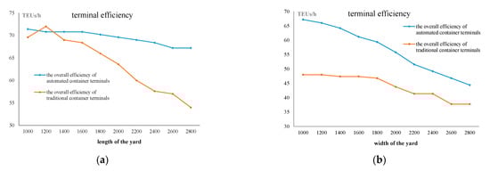
Figure 6.
The terminal efficiency with various yard size. (a) Changing the length of the yard. (b) Changing the width of the yard.
5. Conclusions
Traditional container terminals usually use a horizontal yard layout, while automated container terminals usually use a vertical yard layout. The two types of yard layout lead to different vehicle travel routes, the handling interface points of vehicles and yard cranes, and the yard cranes travel routes. These differences will finally affect the terminal efficiency, such as yard utilization, terminal throughput, construction cost, etc. To quantify these indicators, this paper compares the operation efficiency of the horizontal yard layout of the traditional container terminals with that of the vertical layout of the automated container terminals. We use an analytic method to model the vehicle travel distance and the yard crane travel distance with various yard sizes. Then, the terminal efficiency is evaluated from the overall operations by a queuing network. In the experiment studies, we first evaluated the indicators of the two types of yard layout, respectively. Then, we change the length and width of the yard to evaluate the efficiency for different container terminal sizes. From the analysis results, we can find that the vehicle travel distance is shorter with a vertical yard layout, but the yard crane travel distance is longer in some cases. The overall efficiency of the terminal varies in different yard sizes because various yard layouts lead to different construction costs; terminal operators can choose a proper yard layout before the automated container terminal is reconstructed.
In future studies, more types of yard layout can be modelled, and the analysis results may contribute to the terminal design. Researchers can also optimize the schedules in the different types of yard layout.
Author Contributions
Conceptualization, X.Z., Y.G. and B.L.; methodology, X.Z. and Y.G.; software, X.Z. and Y.G.; validation, Y.G. and B.L.; writing—original draft preparation, X.Z., Y.Y. and Y.G.; writing—review and editing, B.L.; visualization, B.L. and Y.Y.; funding acquisition, X.Z. All authors have read and agreed to the published version of the manuscript.
Funding
This research was funded by the National Natural Science Foundation of China (NSFC), grant number 71901005 and the Social Science Program of Beijing Municipal Education Commission, grant number SM202010011008.
Institutional Review Board Statement
Not applicable.
Informed Consent Statement
Informed consent was obtained from all subjects involved in the study.
Data Availability Statement
Not applicable.
Acknowledgments
The authors would like to thank the editors and referees for their careful reading and constructive suggestions.
Conflicts of Interest
The authors declare no conflict of interest.
References
- Yu, W.; Egbelu, P.J. Scheduling of inbound and outbound trucks in cross docking systems with temporary storage. Eur. J. Oper. Res. 2018, 4, 377–396. [Google Scholar] [CrossRef]
- Nossack, J.; Pesch, E. Atruck scheduling problem arising in intermodal container transportation. Eur. J. Oper. Res. 2013, 230, 666–680. [Google Scholar] [CrossRef]
- Liu, C.I.; Jula, H.; Vukadinovic, K.; Ioannou, P. Automated guided vehicle system for two container yard layouts. Transp. Res. Part C Emerg. Technol. 2004, 12, 349–368. [Google Scholar] [CrossRef]
- Kemme, N. Effects of storage block layout and automated yard crane systems on the performance of seaport container terminals. OR Spectr. 2012, 34, 563–591. [Google Scholar] [CrossRef]
- Meller, R.D.; Gau, K.-Y. The facility layout problem: Recent and emerging trends and perspectives. J. Manuf. Syst. 1996, 15, 351–366. [Google Scholar] [CrossRef]
- Kim, K.H.; Park, Y.-M.; Jin, M.-J. An optimal layout of container yards. OR Spectr. 2008, 30, 675–695. [Google Scholar] [CrossRef]
- Tierney, K.; VoB, S.; Stahlbock, R. A mathematical model of inter-terminal transportation. Eur. J. Oper. Res. 2014, 235, 448–460. [Google Scholar] [CrossRef]
- Lee, B.K.; Kim, K.H. Optimizing the yard layout in container terminals. OR Spectr. 2013, 35, 363–398. [Google Scholar] [CrossRef]
- Abu Aisha, T.; Ouhimmou, M.; Paquet, M.; Montecinos, J. Developing the seaport container terminal layout to enhance efficiency of the intermodal transportation system and port operations—Case of the Port of Montreal. Marit. Policy Manag. 2021, 49, 181–198. [Google Scholar] [CrossRef]
- Budiyanto, M.A.; Huzaifi, M.H.; Sirait, S.J.; Prayoga, P.H.N. Evaluation of CO2 emissions and energy use with different container terminal layouts. Sci. Rep. 2021, 11, 5476. [Google Scholar] [CrossRef] [PubMed]
- Guppa, A.; Roy, D.; DE Koster, R.; Parhi, S. Optimal stack layout in a sea container terminal with automated lifting vehicles. Int. J. Prod. Res. 2017, 55, 3747–3765. [Google Scholar]
- Li, X.; Peng, Y.; Huang, J.; Wang, W.; Song, X. Simulation study on terminal layout in automated container terminals from efficiency, economic and environment perspectives. Ocean. Coast. Manag. 2021, 213, 105882. [Google Scholar] [CrossRef]
- Gharehgozli, A.; Zaerpour, N.; de Koster, R. Container terminal layout design: Transition and future. Marit. Econ. Logist. 2020, 22, 610–639. [Google Scholar] [CrossRef]
- Bjerkan, K.Y.; Seter, H. Reviewing tools and technologies for sustainable ports: Does research enable decision making in ports? Transp. Res. Part D Transp. Environ. 2019, 72, 243–260. [Google Scholar] [CrossRef]
- Bassan, S. Evaluating seaport operation and capacity analysis—Preliminary methodology. Marit. Policy Manag. 2007, 34, 3–19. [Google Scholar] [CrossRef]
- Chu, C.; Huang, W. Determining container terminal capacity on the basis of an adopted yard handling system. Transp. Rev. 2005, 25, 181–199. [Google Scholar] [CrossRef]
- Vidovic, M.; Kim, K.H. Estimating the cycle time of three-stage material handling systems. Ann. Oper. Res. 2006, 144, 181–200. [Google Scholar] [CrossRef]
- Roy, D.; Gupta, A.; Koster, R.B.M.D. Stochastic modeling of unloading and loading operations at a container terminal using automated lifting vehicles. Eur. J. Oper. Res. 2018, 266, 895–910. [Google Scholar] [CrossRef]
Disclaimer/Publisher’s Note: The statements, opinions and data contained in all publications are solely those of the individual author(s) and contributor(s) and not of MDPI and/or the editor(s). MDPI and/or the editor(s) disclaim responsibility for any injury to people or property resulting from any ideas, methods, instructions or products referred to in the content. |
© 2023 by the authors. Licensee MDPI, Basel, Switzerland. This article is an open access article distributed under the terms and conditions of the Creative Commons Attribution (CC BY) license (https://creativecommons.org/licenses/by/4.0/).