Time Series Forecast of Cooling Demand for Sustainable Chiller System in an Office Building in a Subtropical Climate

Abstract

Commercial buildings can take up one-third of the energy related carbon emissions. There is limited research on forecasting cooling demands to evaluate sustainable air conditioning systems under climate change. This paper develops a simplified cooling demand model based on the time series of climatic and architectural variables to analyze carbon reduction by a sustainable chiller system. EnergyPlus is used to simulate hourly cooling demands of a hypothesized high-rise office building in Hong Kong under a change of architectural parameters and future climate conditions. An hourly cooling demand model with R² above 0.9 is developed with inputs of the window-to-wall ratio, outdoor air enthalpy, global solar radiation, wind speed and their two steps ahead. The validated model is then used to analyze carbon reduction potentials by free cooling and a full variable speed chiller system. The low carbon technologies reduce carbon emissions by over 20% with but the reduction shrinks to 2.51–4.93% under future climate conditions. The novelty of this study is the simplified cooling demand model based on the time series of climatic and architectural variables. The significances of this study are to quantify carbon reduction by a sustainable chiller system under climate change and to appeal for more carbon reduction technologies for carbon neutrality.

1. Introduction

One third of the energy related carbon emissions can be caused by commercial buildings [1]. To achieve carbon neutrality in the coming decades, it is important to implement low to zero carbon technologies in building envelopes, lighting systems and heating, ventilation and air conditioning (HVAC) systems [2]. HVAC systems generally take up the highest proportion of energy consumption in the buildings and, hence, offer high opportunity for carbon reduction. Chiller systems within HVAC systems produce cooling energy with significant energy use. The energy performance of chiller systems depends on how they operate with optimal settings to meet varying cooling demands [3]. When building management systems are installed, extensive operating and energy data can be logged at 15-min to 1-h intervals to evaluate energy saving opportunities for building services systems. On the other hand, simulation data generated from common building energy simulation tools such as EnergyPlus [4], TRNSYS [5] and DOE-2 [6] can be used to analyze cooling demand profiles and system performance under optimal design alternatives [7].

It is difficult and even challenging to use physical models for thermal and energy analyses based on numerous parameters in architectural and building system designs. Alternatively, data-driven models are increasingly used to forecast cooling demands and optimize system operation.

Table 1. Some existing data-driven models and optimization algorithms.

Reference	Research Problem	Variables Optimized	Optimization Algorithm
Huang et al. [8]	Cooling demand forecast; Min. system energy consumption	Temperatures of chilled water and cooling water	Support vector regression for demand forecast
Torres et al. [9]	Chiller system energy prediction and min. life cycle cost	Chiller combination; cooling capacity distribution	Parametric study
Olszewski [10]	Energy saving by variable speed drive	Coefficient of performance (COP)	Parametric study
Xue et al. [11]	Min. chiller power is a function of part-load ratio (PLR)	PLR	Improved sparrow search algorithm
Cai et al. [12]	Min. chiller power is a function of PLR	PLR	Improved imperialist competitive algorithm
Lain et al. [13]	Min. chiller power is a function of PLR	PLR	Backward modelling approach
Gao et al. [14]	Min. chiller power is a function of PLR	PLR	Improved parallel particle swarm optimization algorithm
Yu et al. [15]	Min. chiller power is a function of PLR	PLR	Distributed framework
Sohrabi et al. [16]	Min. chiller power is a function of PLR	PLR	Exchange market algorithm
Zheng and Li [17]	Min. chiller power is a function of PLR	PLR	Improved invasive weed optimization algorithm
Saeedi et al. [18]	Min. chiller power is a function of PLR	PLR	General algebraic modelling system optimization
Nedjah et al. [19]	Min. chiller power and cooling tower power	COP and tower heat exchange efficiency	Swarm intelligence-based multi-objective optimization

summarizes previous research problems with data-driven models and the optimization algorithms.

Huang et al. [8] used support vector regression to develop a cooling-demand model with an R² of around 0.9 and quantified an energy saving of 12.4% based on an optimal control strategy for the chiller system. Variables at each time point were assumed to be independent and the part-load performance of the chillers were not illustrated. Indeed, operating conditions of a real system depend on controlled variables in previous time points and their set points. Torres et al. [9] performed statistical analyses to ascertain the correlation of the total energy consumption and life-cycle cost with system parameters in terms of the number of chillers, the total capacity installed and load distribution among chillers. Yet, the full variable speed control for chillers, pumps and cooling towers was not considered. Olszewski [10] ascertained the superior performance of variable speed chillers to handle part-load conditions compared with common on/off controlled chillers. Some recent studies in references [11,12,13,14,15,16,17,18] focus on the optimum loading of multiple chillers with various optimization algorithms. The chiller coefficient of performance (COP)—cooling capacity output in kW over chiller electric power input in kW—was expressed as a function of part-load ratio (PLR), only without considering the temperatures of chilled water and condenser water. The power of chilled water pumps, condenser water pumps and cooling tower fans were disregarded in the optimization problems. Furthermore, the interaction between the system load and climatic variables was ignored, which imposes uncertainty in simulating the actual system performance under the constraint of ambient conditions. Nedjah et al. [19] used swarm intelligence with multi-objective optimization for cooling towers and chillers to achieve power savings of 9.48%. The optimum problem did not consider the power trade-off of condenser pumps and the variation of chiller loads with the outdoor wet bulb temperatures.

Overall, past studies do not explore a simplified model which can predict hourly cooling demands for building energy simulation under future climate conditions. The interdependence of cooling demands in successive time points is ignored. Most past chiller system models do not comprehensively consider the power components of chillers, chilled water pumps, condenser water pumps and cooling tower fans and their optimum settings to minimize electricity use.

There is limited comprehensive analysis on three related research problems: (1) forecasting cooling demands based on architectural parameters and weather data and their time steps ahead; (2) developing a simplified model to predict cooling demand profiles under climate change; (3) investigating carbon reduction potentials of free cooling and a full variable speed chiller system operating for cooling demands under future climate conditions. To address these research problems in one go, the aim of this study is to develop a time series cooling-demand model to evaluate a sustainable chiller system for an office building under climate change. EnergyPlus [4] will be used to simulate hourly cooling demand profiles of a reference office building and its HVAC system in Hong Kong. A simplified cooling-demand model will be developed based on time series of weather data and architectural parameters. The accuracy of the model will be examined for cooling demands under future climate conditions. An estimation will be made on how free cooling and a full variable speed chiller system reduce carbon emissions based on cooling-demand profiles under climate change. The novelty of this study is the simplified cooling-demand model based on the time series of climatic and architectural variables. The significances of this study are to quantify carbon reduction by a sustainable chiller system under climate change and to appeal for more carbon reduction technologies for carbon neutrality.

2. Materials and Methods

2.1. Descriptions of the Building and Its HVAC System

The studied building is a hypothesized high-rise office building with 40 floors, a height of 128 m and a gross floor area of 51,840 m². Each floor has dimensions of 36 m × 36 m with a non-air-conditioned core area of 225 m². Such a building configuration is considered as a stereotype to benchmark the energy performance of typical office buildings in Hong Kong [20]. Bao et al. [21] used this configuration to develop an integrated part load value for chillers serving office buildings. A similar configuration with slightly different floor dimensions was considered to examine the accuracy of modelling the energy use of office buildings in Hong Kong [22]. The curtain wall system is applied with U-values of 0.735 W/m² °C for the roof and 2.326 W/m² °C for opaque walls. There is no external shading and the glass shading coefficient is 0.35. Based on a survey on existing office buildings in Hong Kong [23], the common window-to-wall ratio (WWR) range is 0.4 to 0.8 and 0.4 is considered as the baseline. Regarding indoor environmental parameters, the indoor temperature and relative humidity are set at 24 °C and 50%, respectively. The ventilation rate is based on 10 L/s per person and an occupancy density of 9 m² per person. The lighting power density is 15 W/m² and the equipment power density is 25 W/m² in the calculation of internal heat gains. All the parameters are inputted into building description modules in EnergyPlus to simulate hourly cooling demands throughout the year.

The HVAC system operates 8 a.m.–7 p.m. on Mondays to Fridays and 8 a.m.–1 p.m. on Saturdays.

Table 2. Key specifications of the HVAC systems at the baseline and low carbon design.

Parameter	Conventional Design (Baseline)	Low Carbon Design
Chiller system
Chiller type and capacity control	Constant speed centrifugal chiller with inlet guide vane	Variable speed centrifugal chiller
Number of chiller and pump sets	4	4
Full load COP	5.6	6.5
Integrated part-load value (IPLV)	6.25	11.5
Chilled water design set point (°C)	7	7
Primary-loop pump	Constant speed (rated 65.04 kg/s and 15 kW)	Variable speed (rated 65.04 kg/s and 30 kW)
Secondary-loop pump	Variable speed (rated at 65.04 kg/s and 15 kW)	Not applicable
Cooling tower fan	High/low speed (rated at 24.91 m3/s and 3 kW)	Variable speed (rated at 24.91 m3/s and 3 kW)
Condenser water pump	Constant speed (rated at 76.66 kg/s and 19.53 kW)	Variable speed (rated at 75.05 kg/s and 76.49 kW)
Air side system	Constant air volume (CAV)	Constant air volume (CAV)
Total airflow and power	142.56 m3/s and 203.66 kW	142.56 m3/s and 203.66 kW
Minimum airflow fraction	0.5	0.5
Fan motor efficiency	0.9	0.9

summarizes key specifications used in system modules in EnergyPlus. The COP and IPLV of the two types of chillers are based on a study report on the application of high-efficiency chillers [24].

2.2. Simulation of Chiller System

Chiller modelling equations used in EnergyPlus are presented by Equations (1)–(6) [25]. The electric power input (P_E) in Equation (1) is calculated based on three calibrated variables for full-load capacity (CAPFL), full-load electric power input (EIRFT) and part-load electric power input (EIRPLR). The Q_r and COP_r are the rated cooling capacity in kW and COP at full load, respectively. Instead of considering only the part-load ratio (PLR), the chilled water supply temperature (T_chs) and the condenser water leaving temperature (T_cdl) are included in the calibration. This helps capture the variation of part-load performance when optimizing T_chs and T_cdl under variable speed control. For a given cooling capacity (Q_E) at part-load operation in Equation (5), the COP is given by Equation (6).

Table 3. Parameters and coefficients in chiller models.

Parameter or Coefficient	Constant Speed	Variable Speed
Qr (kW) (nominal capacity)	1526	1526
COPr (nominal full-load COP)	5.6	6.5
a0	−0.2176	−0.2176
a1	−0.0494	−0.0494
a2	8.70 × 10−5	8.70 × 10−5
a3	0.09612	0.09612
a4	−0.00203	−0.00203
a5	0.00254	0.00254
b0	−0.0199	−0.0199
b1	−0.07848	−0.07848
b2	0.00194	0.00194
b3	0.07123	0.07123
b4	−9.17380 × 10−4	−9.17380 × 10−4
b5	−0.00058	−0.00058
c0	0.35161	0.70911
c1	0.00921	−0.03101
c2	−2.382325 × 10−5	8.06574 × 10−4
c3	0.12232	−0.39730
c4	−0.18201	1.23732
c5	−0.00784	−0.01426

summarizes the parameters and coefficients used to model chillers with constant speed and variable speed controls. The coefficients are not from default models in EnergyPlus. The performance characteristics of the constant speed chiller belong to a commercial chiller fitted and validated by Monfet and Zemeureanu [25]. The coefficients in EIRPLR of the variable speed chiller were fitted based on performance data reported by Beitelmal and Patel [26].

$${\mathrm{P}}_E=Q_r(\mathrm{C}\mathrm{A}\mathrm{P}\mathrm{F}\mathrm{L})(\frac{1}{{COP}_r})(\mathrm{E}\mathrm{I}\mathrm{R}\mathrm{F}\mathrm{L})(\mathrm{E}\mathrm{I}\mathrm{R}\mathrm{P}\mathrm{L}\mathrm{R})$$

(1)

$$\mathrm{C}\mathrm{A}\mathrm{P}\mathrm{F}\mathrm{L}=a_0+a_1{T}_{chs}+a_2{T}_{chs}^2+a_3{T}_{cdl}+a_4{T}_{cdl}^2+a_5{T_{chs}·T}_{cdl}$$

(2)

$$\mathrm{E}\mathrm{I}\mathrm{R}\mathrm{F}\mathrm{L}=b_0+b_1{T}_{chs}+b_2{T}_{chs}^2+b_3{T}_{cdl}+b_4{T}_{cdl}^2+b_5{T_{chs}·T}_{cdl}$$

(3)

$$\mathrm{E}\mathrm{I}\mathrm{R}\mathrm{P}\mathrm{L}\mathrm{R}=c_0+c_1{T}_{cdl}+c_2{T}_{cdl}^2+c_{3}PLR+c_4{PLR}_{}^2+c_5{T}_{cdl}·PLR$$

(4)

$${\mathrm{Q}}_E=PLR{·Q}_r\left(\mathrm{C}\mathrm{A}\mathrm{P}\mathrm{F}\mathrm{L}\right)$$

(5)

$${\mathrm{C}\mathrm{O}\mathrm{P}=\mathrm{Q}}_E/{\mathrm{P}}_E$$

(6)

Figure 1 shows the modelled COP at different combinations of PLR and T_cdl under constant speed and variable speed controls. The constant speed chiller has the maximum COP at a PLR of 0.8, while the maximum COP of the variable speed chiller is shifted to a PLR of 0.6.

Based on the optimal PLRs with the maximum COPs, Figure 2 shows how one to four chillers are staged to match different system cooling demands. When the PLR of constant speed chillers exceeds one, one more chiller should be switched on to meet the increasing cooling demand, while prolonging a high PLR with a high COP. The number of chillers operating will be kept minimal at different system cooling demands to minimize the total power of chillers, pumps and cooling tower fans. On the other hand, more variable speed chillers operate frequently near a PLR of 0.6 to achieve the highest efficiency of the chillers, pumps and cooling tower fans at lower speed. All the four variable speed chillers are staged when the cooling demand increases from 2900 kW.

In the sub-tropical climate, if the outdoor air enthalpy (h_o) is below the required indoor air enthalpy, the airside system can supply more outdoor air to reduce the cooling demand handled by the chiller system. Given the total supply airflow rate of 142.56 m³/s and the indoor air enthalpy of 47.9 kJ/kg to maintain 24 °C and 50% relative humidity, free cooling can compensate for one chiller capacity rated at 1526 kW when h_o drops to 39 kJ/kg. It is possible that no chiller needs to operate in winter months with h_o below 39 kJ/kg. The reduction of cooling demand (CD_r) in kW on the chiller system is given by Equation (7), where V_s is the total supply airflow rate in m³/s, ${\mathsf{\rho }}_a$ is the air density of 1.2 kg/m³ and h_i is the indoor air enthalpy of 47.9 kJ/kg:

$${\mathrm{C}\mathrm{D}}_r=V_s{·\mathsf{\rho }}_a(h_i-h_o)$$

(7)

2.3. Simulation Scenarios for Architectural Parameters and Weather Data

The architectural parameter change is the window-to-wall ratio (WWR) as it strongly influences the solar heat gain and, hence, the thermal performance of the building envelope. The WWR values of 0.4 (baseline), 0.5, 0.6, 0.7 and 0.8 are considered in the cooling demand simulation. To simulate the baseline of building electricity use, the typical meteorological year (TMY) for Hong Kong is considered [27]. Yet, the typical months used to compile the TMY weather data are based on 1979–2003, which cannot reflect weather conditions under climate change. The weather generator program CCWorldWeatherGen [28] was used to produce weather data in 2020 (representing 2010–2039), 2050 (representing 2040–2069) and 2080 (representing 2070–2099). The weather data files were generated in the epw format for simulation in EnergyPlus. The future weather data were used to investigate the impacts of carbon emissions by the studied building. The weather generation involves shifting and stretching the TMY data based on general circulation models (GCMs) [29] used for global climate projection. The assumptions involve medium-high emissions scenarios (A2) with business-as-usual development by human emissions [30]. The morphed hourly outdoor temperature shifts by 0.62–0.68 °C with stretching of −0.01–0.01 in 2020, 1.40–2.16 °C with stretching of −0.08–0.00 in 2050, and 2.38–3.69 °C with stretching of −0.12–0.02 in 2080, in relation to that in TMY. More explanation on the weather generation process can be found at Yu et al. [31]. The morphed hourly weather data can be considered as an interim and feasible source to predict building energy consumption while the TMY data are not yet revamped to adapt to climate change scenarios.

Figure 3, Figure 4, Figure 5 and Figure 6 show the modelled data of major climatic variables in 2020, 2050 and 2080 against the TMY. They are compiled in the epw format required in EnergyPlus to perform cooling demand simulation. Under climate change, the hourly outdoor temperature rises by an average of 0.4–2.3 °C over the three future periods. This is attributed to the impact of global warming. The hourly outdoor air enthalpy increases by an average of 0.88–6.96 kJ/kg over three future climate conditions. The increase of the outdoor temperature and enthalpy will cause more heat gains transmitted from ventilation and building envelope and, hence, will increase the hourly cooling demands. The hourly global horizontal radiation tends to increase in winter months and decrease in summer months in future climate conditions. This will bring a drop of the solar heat gain at the peak cooling demand, but will increase the moderate cooling demands in mild seasons. The variation of hourly wind speeds in 2020, 2050 and 2080 follows roughly the same pattern as shown in the TMY.

2.4. Descriptions on Simulation Outputs and Carbon Emissions with Low Carbon Chiller System

Parameters of the building, its systems and weather data were compiled and put in simulation modules in EnergyPlus. The outputs involve hourly data of cooling demands and electricity uses of the HVAC system, lighting system and other electrical systems. Since EnergyPlus does not contain default modules to simulate a free cooling and full variable speed chiller system, the associated energy consumption was computed separately based on the cooling demand profiles under three future climate conditions. To facilitate this computation by the chiller model, a simplified time series cooling-demand model was developed, which includes essential climatic variables and the WWR as the input variables.

Two power companies in Hong Kong have different carbon emission patterns in electricity generation. An average carbon emission factor of 0.6 kgCO₂-e per kWh [32] was used to convert the electric use in kWh into carbon emissions in kgCO₂-e. The annual electricity uses of the chiller system with constant speed and variable speed controls were compared to assess whether the carbon reduction facilitates a drop of 50% in the decarbonazation strategy in Hong Kong’s climate action plan 2050 [33].

3. Development of a Times Series Cooling-Demand Model

3.1. Data Sources for Model Development

In building description modules in EnergyPlus, the change of architectural parameters involves five values of WWRs: 0.4, 0.5, 0.6, 0.7 and 0.8. There are four weather files: TMY, 2020, 2050 and 2080. Data of hourly cooling demands with the TMY were used as the training set. The testing sets involve the associated data simulated with weather files in 2020, 2050 and 2080. The mathematical expression of the time series regression model is given by Equation (8), where at each hourly time point t, y_t is the output, β_o is the constant, β_i,t is the coefficient of the input variable x_i,t and e_t is the error term. Different from the typical regression model, one step ahead (x_i,t−1) and two steps ahead (x_i,t−2) of x_i,t are considered to improve the prediction accuracy. According to Wan et al. [34], the cooling demand forecast can be 1-h step ahead due to the thermal storage effect of the building envelope when converting external heat gains into cooling demands in indoor spaces. The 2-h step ahead is considered here because the successive change of chiller operating status can likely last for 2 h [35].

$${\mathrm{y}}_t={{\beta }_o+\sum ({\beta }_{i,t}x}_{i,t}+{{\beta }_{i,t-1}x}_{i,t-1}+{{\beta }_{i,t-2}x}_{i,t-2})+e_t$$

(8)

The output y_t is the hourly cooling demand (CD) in kW in the time series model. The input variables x_i,t involve one architectural variable (WWR) and four hourly climatic variables: outdoor dry bulb temperature (t_o) in deg. C; outdoor air enthalpy (h_o) in kJ/kg; global horizontal radiation (GHR) in W/m²; and wind speed (v) in m/s. Descriptive statistics of the climatic variables are shown in

Table 4. Descriptive statistics of climate variables.

Variable	Minimum	Maximum	Mean	Std. Deviation
to (°C)	10.10	32.80	23.7600	5.37159
ho (kJ/kg)	17.98	90.38	60.7305	17.79912
GHR (W/m2)	0.00	972.00	3.0401E2	251.20434
v (m/s)	0.50	10.00	3.3069	1.67185

. These climatic variables are found to be essential in the cooling demand calculation [3]. To ensure model’s reliability, Pearson correlation coefficients among the input variables and variance inflection factors (VIFs) were calculated to detect multicollinearity. One variable was selected among highly correlated variables to maintain a high model accuracy while keeping all the VIFs below 5.

The coefficient of determination (R²) given by Equation (9) was used to measure how well the model predicts the observations of y_i. ${\widehat{y}}_i$ is the predicted $y_i$ and $\stackrel{-}{y}$ is the mean of $y_i$ for a sample size n. A R² of 1 means the model can predict all observations accurately. An R² of 0.8 indicates a model with very high accuracy as 80% of the variation of the predicted values can be explained by the change of observations.

$$R^2=\frac{\sum _{i=1}^n{({\widehat{y}}_i-\stackrel{-}{y})}^2}{\sum _{i=1}^n{(y_i-\stackrel{-}{y})}^2}$$

(9)

4. Results and Discussion

4.1. Cooling Demand Profiles at Various Combinations of WWR and Weather Data

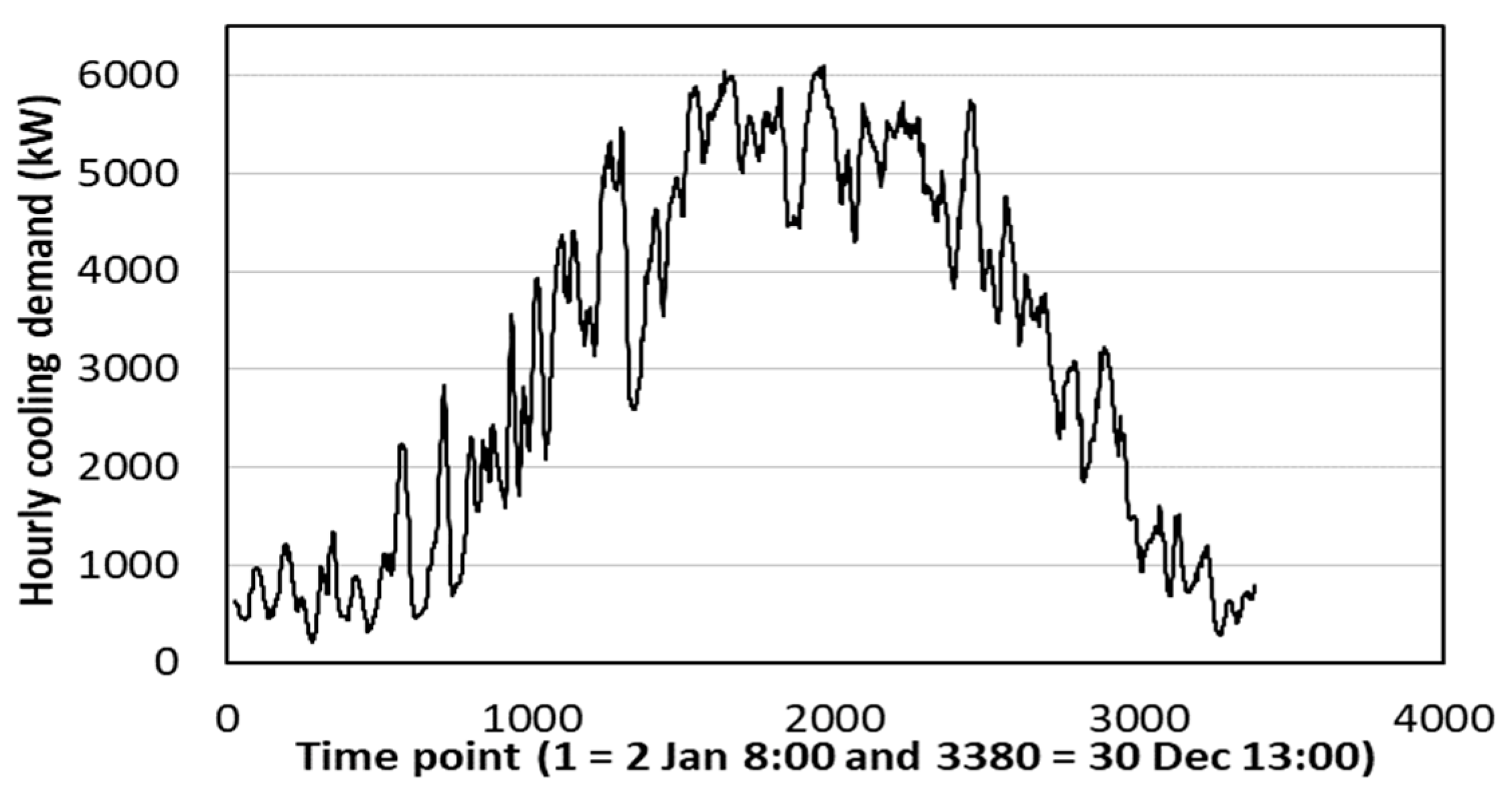
Simulation results from EnergyPlus were processed with changes of WWRs of 0.4, 0.5, 0.6, 0.7 and 0.8 and four sets of weather data in TMY, 2020, 2050 and 2080. Figure 7 shows the hourly cooling-demand profile in the base case with a WWR of 0.4 and TMY. There are 3380 time points based on operating hours of the HVAC system in the year. The lowest cooling demand occurs in January and the peak cooling demand occurs in July. The cooling demand is non-zero in winter months with outdoor temperatures below 20 °C because there are solar heat gains from windows and internal loads from occupants and equipment. The seasonal variation of the profile generally follows the profiles of the outdoor temperature and outdoor air enthalpy given in Figure 3 and Figure 4.

Figure 8 gives the percentage changes of hourly cooling demands in January and July from the base case with higher WWRs from 0.5 to 0.8. For the bottom tier of cooling demands in January, the higher WWRs result in higher percentage increases of the cooling demand. For the top pier of cooling demands in July, the percentage increase is up to 12.8% in the hourly cooling demands with higher fluctuation in successive hours.

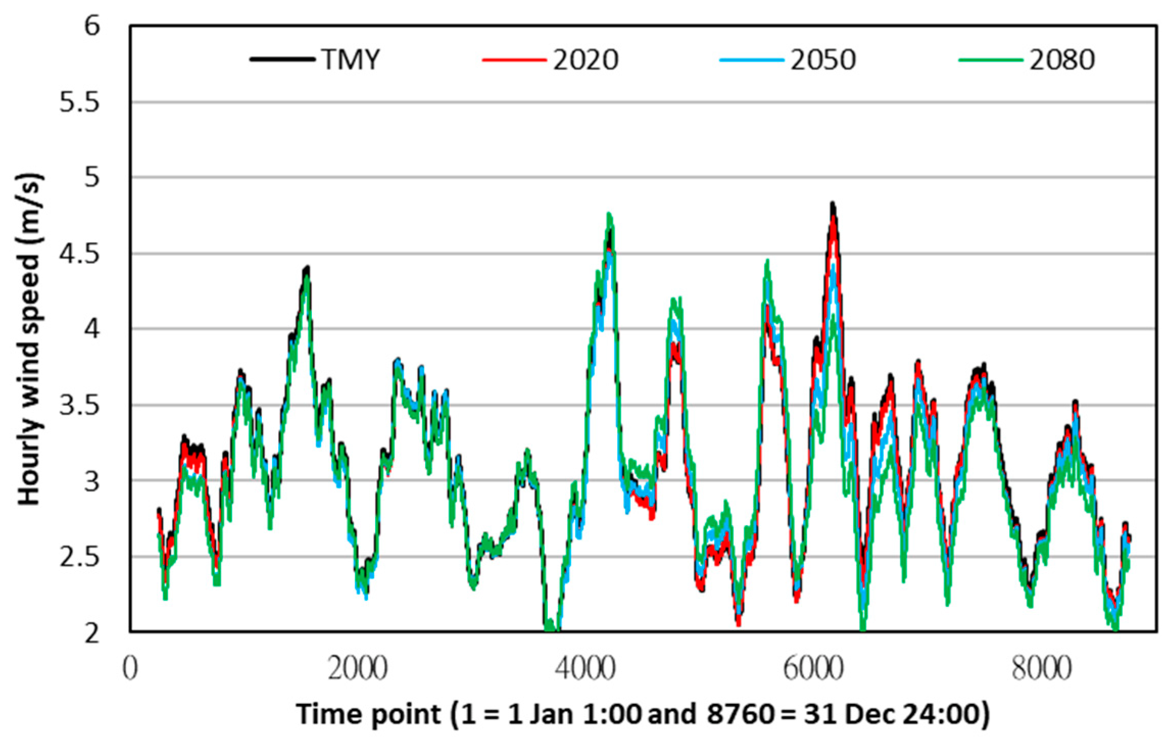
Figure 9 shows the increase of hourly cooling demands with a WWR of 0.4 in 2020, 2050 and 2080 in relation to the TMY. Light cooling demands in winter months can increase by 17.9–102.8% with time points 1–544 and 2820–3380. On the other hand, the upper cooling demands increase slightly by 9.0–21.6% in summer months with time points 1106–2258. When considering the extension of cooling demands in the future climate, the chiller system capacity should not be oversized by more than one-fourth of the peak cooling demand to avoid operating chillers at low PLRs under light cooling demands.

Overall, simulation results of cooling demand profiles show various daily variations under five WWRs and four weather conditions. The data sets are comprehensive to train and test the time series cooling-demand model for further analysis of carbon reduction by free cooling and a full variable speed chiller system.

4.2. Time Series Cooling-Demand Model and Its Validation

Pearson correlation coefficients are presented in

Table 5. Pearson correlation coefficients of input variables.

Variable	WWR	to (°C)	ho (kJ/kg)	GHR (W/m2)	v (m/s)
WWR	1	0.00000	0.00000	0.00000	0.00000
to (°C)	0.00000	1	0.95224	0.35697	0.06113
ho (kJ/kg)	0.00000	0.95224	1	0.19702	0.03265
GHR (W/m2)	0.00000	0.35697	0.19702	1	0.18360
v (m/s)	0.00000	0.06113	0.03265	0.18360	1

for input variables of WWR, t_o, h_o, GHR and v described in Section 3.1. The variables t_o and h_o are found to be highly correlated with a correlation coefficient of 0.95224. Based on the warm-humid climate in Hong Kong with a minor variation in relative humidity, the correlation between t_o and h_o follows generally the psychrometric properties of air. Their selection in the final model is based on the variance inflation factors (VIFs) and the change of R² when dropping out either t_o or h_o.

Table 6. Statistical results of regression model.

Variable	Unstandardized Coefficients		Standardized Coefficients	T	Sig.	Collinearity Statistics
	B	Std. Error	Beta			Tolerance	VIF
(Constant)	−4549.6914	35.0864		−129.6710	0.0000
WWR	333.1573	34.1988	0.0236	9.7418	0.0000	1.0000	1.0000
to	146.9705	3.5759	0.3952	41.1000	0.0000	0.0634	15.7727
ho	59.7808	1.0282	0.5327	58.1398	0.0000	0.0698	14.3184
GHR	0.8210	0.0241	0.1032	34.0536	0.0000	0.6384	1.5665
v	−20.83078	2.9430	−0.0174	−7.0780	0.0000	0.9663	1.0349

shows the statistical results of a general regression model without one or two steps ahead. The model has an R² of 0.901, which indicates 90.1% of the change of cooling demand can be explained by the variation of input variables. Yet, the VIFs of above 10 are observed in t_o and h_o, which confirms their high correlation in the model. Dropping out t_o and h_o individually from the model gives an R² of 0.891 and 0.881, respectively. The preference of including h_o and excluding t_o in the model is also supported by a high standardized coefficient of 0.533 for h_o compared with 0.395 for t_o. The VIFs vary between 1.000–1.182, which are well below 5 when excluding t_o from the five input variables. The time series regression model will be developed based on the input variables of WWR, h_o, GHR and v. Most building management systems monitor only the outdoor temperature and no other properties of outdoor air. While t_o can be measured and logged directly, the higher priority of h_o ascertains a need of monitoring the outdoor air enthalpy by two climatic variables (e.g., t_o and relative humidity) to predict the change of cooling demands. Indeed, relative humidity itself has a very low correlation with the cooling demand. It is more preferable to use h_o, which captures the heat gained from the water vapor of outdoor air compared with using t_o solely. When free cooling is applied, the outdoor air enthalpy is highly correlated with the indoor air enthalpy, which has a stronger impact on the thermal acceptability than other thermal parameters [36].

Table 7. Statistical results of time series regression model with one step ahead.

Variable	Unstandardized Coefficients		Standardized Coefficients	t	Sig.
	B	Std. Error	Beta
(Constant)	−3657.3869	26.4992		−138.0189	0.0000
WWR	333.1573	31.8950	0.0236	10.4454	0.0000
ho,t	24.2267	3.1887	0.2159	7.5977	0.0000
GHRt	−0.2352	0.0358	−0.0296	−6.5717	0.0000
vt	−32.3596	4.5714	−0.0271	−7.0787	0.0000
ho,t−1	74.5720	3.1724	0.6670	23.5063	0.0000
GHRt−1	2.0356	0.0358	0.2537	56.8044	0.0000
vt−1	−0.2924	4.5045	−0.0002	−0.0649	0.9483

and

Table 8. Statistical results of time series regression model with two steps ahead.

Variable	Unstandardized Coefficients		Standardized Coefficients	t	Sig.
	B	Std. Error	Beta
(Constant)	−3670.4868	25.7575		−142.5017	0.0000
WWR	333.1573	30.8957	0.0236	10.7833	0.0000
ho,t	22.0839	3.1313	0.1968	7.0526	0.0000
GHRt	0.4153	0.0404	0.0522	10.2836	0.0000
vt	−19.5087	4.6202	−0.0163	−4.2224	0.0000
ho,t−1	38.2536	4.0880	0.3421	9.3575	0.0000
GHRt−1	0.4886	0.0630	0.0609	7.7513	0.0000
vt−1	−10.3853	5.1242	−0.0088	−2.0267	0.0427
ho,t−2	37.7826	3.1646	0.3388	11.9392	0.0000
GHRt−2	1.1898	0.0409	0.1510	29.1070	0.0000
vt−2	−7.2308	4.5021	−0.0062	−1.6061	0.1083

show statistical results of the time series models with only one step ahead (i.e., the t − 1 term) and two steps ahead (i.e., the t − 1 and t − 2 terms). The R² can be improved from 0.891 to 0.914 with one step ahead and further, to 0.919 with two steps ahead. The h_o and GHR are the most significant variables to model the cooling demand because they are important variables to calculate the ventilation load and solar heat gain from windows. Based on standardized coefficients in Table 8, h_o,t−1 has a heavier weighting than h_o,t and h_o,t−2. GHR_t−2 has the highest weighting compared with GHR_t and GHR_t−1. This corroborates the delayed effect of converting the solar heat gain through the building envelope into the cooling demand. On the other hand, v_t has the highest weighting, but the inclusion of v_t−1 and v_t−1 has no significant effect. Overall, the time series model has improved accuracy with two steps ahead for h_o and GHR. This model development shows the advancement of including previous time steps of explanatory variables.

Equation (10) is established to model the cooling demand (CD_t) at time t with an R² of 0.919 based on the training set. Its validity was further examined by three testing sets under climate conditions in 2020, 2050 and 2080.

Table 9. R² of the testing sets with weather data in 2020, 2050 and 2080.

Testing Sets with Climate Conditions	2020	2050	2080
R2	0.929	0.933	0.929

shows that the values of R² in the testing sets are even higher than 0.919 in the training set. This ascertains the model accuracy under climate change conditions and supports the use of predicted hourly cooling demands to evaluate carbon reduction by the low carbon chiller system using full variable speed control and free cooling.

$$\begin{gathered} {CD}_t=-3681.1705+333.1573\mathrm{W}\mathrm{W}\mathrm{R}+20.7758{\mathrm{h}}_{o,t}+0.4345{\mathrm{G}\mathrm{H}\mathrm{R}}_t-33.3504{\mathrm{v}}_t+40.0640{\mathrm{h}}_{o,t-1} \\ +0.481{\mathrm{G}\mathrm{H}\mathrm{R}}_{t-1}+37.2928{\mathrm{h}}_{o,t-2}+1.1725{\mathrm{G}\mathrm{H}\mathrm{R}}_{t-2} \end{gathered}$$

(10)

This simplified model is a viable tool when a complete set of weather data in the epw format is not available to perform simulation in EnergyPlus. The sensitivity of cooling demands at different WWRs and climatic variables can be assessed directly without changing the building modules in EnergyPlus. Furthermore, the hourly cooling demand profile can be easily generated to evaluate alternative low carbon technologies for HVAC systems that are not yet covered or developed in EnergyPlus system modules.

4.3. Electricity Uses and Carbon Emissions of Chiller System with Conventional and Low Carbon Design

Having found the cooling demand profiles under future climate conditions, the electricity use and carbon emissions are predicted for the chiller system under constant speed control and full variable speed control with free cooling. Other electricity use components for the airside system, lighting system and electrical appliances are skipped in this analysis because they are considered the same at different cooling demand profiles.

Table 10. Annual cooling demands at different combinations of WWRs and climate conditions.

Climate	TMY	2020		2050		2080
WWR	kWh	kWh	% Change	kWh	% Change	kWh	% Change
0.4	9,750,690	10,721,292	9.95	11,598,922	18.95	12,703,046	30.28
0.5	9,873,563	10,866,886	10.06	11,778,949	19.30	12,943,122	31.09
0.6	9,988,159	10,999,101	10.12	11,938,513	19.53	13,160,115	31.76
0.7	10,096,678	11,120,225	10.14	12,083,561	19.68	13,357,118	32.29
0.8	10,202,169	11,234,407	10.12	12,217,879	19.76	13,537,945	32.70

summarizes the annual cooling demands in kWh under all combinations of WWRs and climate conditions. The annual cooling demand in 2080 can increase by 30.28–32.70% from the base case of TMY. This suggests that improving the energy performance of HVAC systems should be strengthened to reduce electricity use to a large extent and, hence, to attain a downward trend in carbon emissions.

Table 11. Annual electricity use in kWh with conventional chiller system at different combinations of WWRs and climate conditions.

Climate	TMY	2020		2050		2080
WWR	kWh	kWh	% Change	kWh	% Change	kWh	% Change
0.4	2,192,072	2,380,612	8.60	2,543,443	16.03	2,755,053	25.68
0.5	2,212,804	2,407,564	8.80	2,581,075	16.64	2,808,490	26.92
0.6	2,234,430	2,433,488	8.91	2,616,870	17.12	2,860,063	28.00
0.7	2,255,259	2,457,312	8.96	2,648,859	17.45	2,908,865	28.98
0.8	2,272,703	2,480,152	9.13	2,681,208	17.97	2,955,204	30.03

shows the annual electricity uses in kWh of the chiller system at different WWRs and climate conditions. The system involves the conventional design with proper staging of constant speed chillers to match different cooling demands. The percentage increase of the annual electricity use follows roughly with the annual cooling demand. To temper the increasing electricity use under future climate conditions, it is important to increase the COP of the chillers, enhance the energy efficiency of the pumps and cooling tower fans and to use free cooling to compensate for the cooling demand as far as possible.

The annual cooling demand data in Table 10 form the base cases without applying free cooling (FC).

Table 12. Annual cooling demands after applying free cooling at different combinations of WWRs and climate conditions.

Climate	TMY		2020		2050		2080
WWR	% Change from Base	% of Time without CD	% Change from Base	% of Time without CD	% Change from Base	% of Time without CD	% Change from Base	% of Time without CD
0.4	−4.96	24.11	5.10	21.15	14.62	16.24	27.07	9.91
0.5	−5.18	23.82	5.02	20.83	14.82	15.92	27.80	9.56
0.6	−5.38	23.40	4.90	20.47	14.90	15.77	28.39	9.32
0.7	−5.58	23.22	4.74	20.30	14.92	15.44	28.85	9.05
0.8	−5.76	22.99	4.56	20.00	14.88	15.15	29.18	8.82

shows the percentage change of annual cooling demands after applying FC from the base cases. Under the TMY, FC enables the annual cooling demand to drop by 4.96–5.76%, depending on the WWRs. In addition, the chiller system can be switched off for 22.99–24.11% of the total operating hours. Under future climate conditions, the potential of applying FC is tempered significantly. In 2080, the percentage reduction of annual cooling demand is limited to 3.21–3.52% in relation to 4.96–5.76% in the TMY. The percentage of time to switch off the chiller system shrinks to 9.05–9.91% in relation to 22.99–24.11% in the TMY.

Table 13. Annual electricity use in kWh with full variable speed chiller system at different combinations of WWRs and climate conditions.

Climate	TMY		2020		2050		2080
WWR	kWh	% Change	kWh	% Change	kWh	% Change	kWh	% Change
0.4	1,816,666	−17.13	1,990,142	−9.21	2,136,866	−2.52	2,299,172	4.89
0.5	1,837,612	−16.96	2,015,407	−8.92	2,168,973	−1.98	2,341,001	5.79
0.6	1,856,355	−16.92	2,038,695	−8.76	2,197,033	−1.67	2,378,271	6.44
0.7	1,874,096	−16.90	2,059,381	−8.69	2,222,237	−1.46	2,411,818	6.94
0.8	1,891,737	−16.76	2,079,210	−8.51	2,244,768	−1.23	2,442,744	7.48

shows how the annual electricity use drops when applying the full variable speed chiller and system in relation to the conventional system. Compared with results in Table 11, the full variable speed chiller system can reduce the annual electricity use by 16.76–17.13% in the TMY and further, by 20.8–22.55% in 2080. The percentage electricity savings are associated with higher equipment efficiency at part-load operation. This suggests that improving the energy performance of the chiller system helps suppress the rising electricity use under future climate conditions. Yet, the percentage drop needs to complement with other low to zero carbon technologies in achieving a proposed energy reduction target of 30–40% in commercial buildings for carbon neutrality in Hong Kong’s climate action plan 2050 [33].

Table 14. Annual electricity use in kWh with full variable speed chiller system and free cooling at different combinations of WWRs and climate conditions.

Climate	TMY		2020		2050		2080
WWR	kWh	% Change	kWh	% Change	kWh	% Change	kWh	% Change
0.4	1,736,387	−20.79	1,912,969	−12.73	2,067,834	−5.67	2,246,990	2.51
0.5	1,754,387	−20.72	1,935,336	−12.54	2,097,166	−5.23	2,287,469	3.37
0.6	1,770,701	−20.75	1,955,142	−12.50	2,122,462	−5.01	2,323,204	3.97
0.7	1,785,404	−20.83	1,972,876	−12.52	2,145,787	−4.85	2,355,307	4.44
0.8	1,800,084	−20.80	1,989,873	−12.44	2,166,646	−4.67	2,384,841	4.93

shows how free cooling can further decrease the annual electricity use with the full variable speed chiller system. Comparing results of percentage changes in Table 13 with Table 14, free cooling brings additional annual electricity savings of 3.66–4.03% in the TMY and 2.38–2.55% in 2080. The shrinkage of electricity savings under future climate conditions is associated with the tempering of reduction in the annual cooling demands as shown in Table 12. These percentage energy savings are much lower than 27% found in a study on the cooling performance of an existing commercial building in Canada [37]. Considering that the percentage changes of the annual electricity use can contribute partly to a proposed energy saving target of 30–40% in commercial buildings, low to zero carbon technologies should be strengthened to the building envelope, other HVAC components, a lighting system, lift and escalator system and photovoltaic system [38,39]. This calls for future research work on simulating various energy saving scenarios for different engineering systems to develop a stereotype of high-rise office buildings in Hong Kong to meet carbon neutrality.

The simplified cooling demand model considers only the basic architectural variable, i.e., the WWR. There are other variables influencing the thermal performance of building envelopes, such as the thermal resistance of envelope materials, the water vapor permeability coefficient, the sealing property, etc. These architectural variables will vary with the building age and the technological advancement of envelope components will interact with the cooling demand profile in the long run. It is worth introducing more architectural variables to enhance the robustness of the cooling demand prediction.

Table 15. Reduction of annual carbon emissions in kgCO₂-e and the percentage drop in relation to total emissions of the studied building.

Climate	TMY		2020		2050		2080
WWR	kgCO2-e	% Drop from Total	kgCO2-e	% Drop from Total	kgCO2-e	% Drop from Total	kgCO2-e	% Drop from Total
0.4	273,412	4.71	280,586	4.84	285,365	4.92	304,838	5.25
0.5	275,050	4.74	283,337	4.88	290,346	5.00	312,613	5.39
0.6	278,237	4.79	287,007	4.95	296,645	5.11	322,115	5.55
0.7	281,913	4.86	290,662	5.01	301,843	5.20	332,134	5.72
0.8	283,571	4.89	294,167	5.07	308,737	5.32	342,218	5.90

gives a summary on the reductions of carbon emissions in kgCO₂-e by using free cooling and full variable speed chiller system at different WWRs and climate conditions. The studied building with a WWR of 0.4 under the TMY has a total electricity consumption is 9,671,391.667 kWh, an energy use intensity of 186.56 kWh/m² and carbon emissions of 5,802,835 kgCO₂-e. The carbon reduction due to the low carbon chiller system operation accounts for 4.84–5.07% in 2020, 4.92–5.32% in 2050 and 5.25–5.90% in 2080. This indicates a need for exploring energy saving opportunities for other building systems, so that the aggregate carbon reduction meets a proposed target of 50% before 2035 in Hong Kong’s climate action plan 2050 [28]. Renewable applications should be widened in high-rise buildings to directly reduce carbon emissions.

This study investigates carbon reduction opportunities mainly from the perspective of building energy efficiency. In fact, the reduction of carbon emission factors from the power supply side is a direct means to suppress carbon emissions for an increasing electricity demand trend under climate change. Widening gas-fired power plants and phasing out coal-fired power plants are the roadmap for power companies in Hong Kong to further reduce the carbon emission factor from the current level of 0.6 kgCO₂-e per kWh.

5. Conclusions and Recommendations

This study develops a simplified cooling-demand model for a high-rise office building in a sub-tropical climate based on the time series of climatic and architectural variables. The model forms a viable tool to assess carbon reduction by a full variable speed chiller system with free cooling under climate change. EnergyPlus is used to simulate hourly cooling demands of a hypothesized high-rise office building in Hong Kong under a change of window-to-wall ratios from 0.4 to 0.8 and climate conditions in the TMY, 2020, 2050 and 2080. The hourly cooling demand model has a very high accuracy with an R² of 0.919 in the training set and 0.929–0.933 in the testing sets. The input variables are the window-to-wall ratio (WWR), outdoor air enthalpy (h_o), global solar radiation (GHR), wind speed (v) and their two steps ahead. Regarding the variable importance for cooling demand prediction, h_o is ranked first, GHR the second, WWR the third and v the last. This addresses a need of monitoring h_o and GHR instead of outdoor temperature only. The h_o can be calculated based on the measured outdoor temperature and relative humidity to facilitate the real-time monitoring of cooling demands in actual chiller systems.

The validated model is used to analyze the electricity use and carbon reduction of a low carbon chiller system with full variable speed control and free cooling against a conventional system. The annual cooling demand in 2080 can increase by 30.28–32.70% from the base case of TMY. Using free cooling enables a minor drop of annual cooling demand by 3.21–3.52% in 2080 and 4.96–5.76% in the TMY. The low carbon chiller system can reduce the annual electricity use by 20.8–22.55% in 2080 and 16.76–17.13% in the TMY. This ascertains the sustainability of using variable speed control and free cooling to achieve more electricity saving under climate change. Yet, other HVAC sub-systems need to complement with other low to zero carbon technologies in achieving a proposed energy reduction target of 30–40% in commercial buildings for carbon neutrality in Hong Kong.

The annual electricity decrease by the low carbon chiller system contributes to a carbon reduction of 4.92–5.32% in 2050 and 5.25–5.90% in 2080. This appeals for exploring more energy-saving opportunities in building systems, so that the aggregate carbon reduction meets a proposed target of 50% before 2035 in Hong Kong. The reduction of carbon emission factors from the power supply side is a direct means to suppress carbon emissions for an increasing electricity demand trend under climate change. Widening gas-fired power plants and phasing out coal-fired power plants are underway to bring a considerable drop in the carbon emission factor from a current level of 0.6 kgCO₂-e per kWh. The carbon reduction target is likely to be achieved under a reduced level of 0.3 kgCO₂-e per kWh with a flattening curve of electricity demand.

This study has some limitations that need to be further examined. First, the simplified cooling demand model considers only WWR as the architectural variable. It is possible to include more parameters about the heat transfer properties of envelope to make the model more generic and robust. Indeed, some changes of architectural parameters will occur over the building age and under the technological advancement. Second, the TMY is likely to be outdated as it was compiled based on weather data in 1979–2003. This may affect the reliability of generating the future weather data in 2020, 2050 and 2080. The TMY should be revamped with weather data in recent decades to reflect better current climate change trends in Hong Kong.

It is important to aggregate more energy saving technologies to meet the 30–40% energy-reduction targets. Future work will be carried out to simulate other energy-saving scenarios with the building envelope, other HVAC components, a lighting system, lift and escalator system and photovoltaic system. Considering that the climate action plans last for several decades, further research work is required about the advancement of the thermal performance of building envelopes in terms of the thermal resistance of the envelope materials, water vapor permeability coefficient, sealing property, etc. Their parameter changes will interact with the change of cooling demands under future climate conditions. Furthermore, the carbon emission trend should be changed when putting forward more stringent policies on electricity use and carbon compensation. The low to zero carbon technologies need to widen renewable applications for over 10% of the overall electricity demand as expected in the climate action plan in Hong Kong. A stereotype high-rise office building with adequate carbon reduction technologies will then be formulated to meet carbon neutrality and to tackle the associated challenges under climate change.

References

1. Lu, M.X.; Lai, J. Review on carbon emissions of commercial buildings. Renew. Sustain. Energy Rev. 2020, 119, 109545. [Google Scholar] [CrossRef]
2. Wan, S.; Ding, G.; Runeson, G.; Liu, Y. Sustainable Buildings’ Energy-Efficient retrofitting: A study of large office buildings in Beijing. Sustainability 2022, 14, 1021. [Google Scholar] [CrossRef]
3. Deng, L.W.; Qiang, W.B.; Peng, C.W.; Wei, Q.P.; Zhang, H. Research on systematic analysis and optimization method for chillers based on model predictive control: A case study. Energy Build. 2023, 285, 112916. [Google Scholar] [CrossRef]
4. U.S. Department of Energy. EnergyPlus Version 22.1.0. 2022. Available online: https://energyplus.net/ (accessed on 20 March 2023).
5. University of Wisconsin. TRNSYS, Transient System Simulation Tool. Available online: https://sel.me.wisc.edu/trnsys/ (accessed on 20 March 2023).
6. James, J.; Hirsch & Associates. Welcome to DOE2.com. Available online: https://www.doe2.com/ (accessed on 20 March 2023).
7. Del Ama Gonzalo, F.; Moreno Santamaría, B.; Montero Burgos, M.J. Assessment of Building Energy Simulation Tools to Predict Heating and Cooling Energy Consumption at Early Design Stages. Sustainability 2023, 15, 1920. [Google Scholar] [CrossRef]
8. Huang, Z.; Chen, X.; Wang, K.; Zhou, B. Air conditioning load forecasting and optimal operation of water systems. Sustainability 2022, 14, 4867. [Google Scholar] [CrossRef]
9. Torres, Y.D.; Gullo, P.; Herrera, H.H.; Torres del Toro, M.; Guerra, M.A.Á.; Ortega, J.I.S.; Speerforck, A. Statistical Analysis of Design Variables in a Chiller Plant and Their Influence on Energy Consumption and Life Cycle Cost. Sustainability 2022, 14, 10175. [Google Scholar] [CrossRef]
10. Pawel Olszewski. Experimental analysis of ON/OFF and variable speed drive controlled industrial chiller towards energy efficient operation. Appl. Energy 2022, 309, 118440. [Google Scholar] [CrossRef]
11. Xue, Z.L.; Yu, J.Q.; Zhao, A.J.; Zong, Y.; Yang, S.Y.; Wang, M. Optimal chiller loading by improved sparrow search algorithm for saving energy consumption. J. Build. Eng. 2023, 67, 105980. [Google Scholar] [CrossRef]
12. Cai, J.Y.; Yang, H.D.; Lai, T.C.; Xu, K.K. A new approach for optimal chiller loading using an improved imperialist competitive algorithm. Energy Build. 2023, 284, 112835. [Google Scholar] [CrossRef]
13. Lian, K.Y.; Hong, Y.J.; Chang, C.W.; Su, Y.W. A novel data-driven optimal chiller loading regulator based on backward modeling approach. Appl. Energy 2022, 327, 120102. [Google Scholar] [CrossRef]
14. Gao, Z.K.; Yu, J.Q.; Zhao, A.J.; Hu, Q.; Yang, S.Y. Optimal chiller loading by improved parallel particle swarm optimization algorithm for reducing energy consumption. Int. J. Refrig. 2022, 136, 61–70. [Google Scholar] [CrossRef]
15. Yu, J.Q.; Liu, Q.T.; Zhao, A.J.; Qian, X.G.; Zhang, R. Optimal chiller loading in HVAC System Using a Novel Algorithm Based on the distributed framework. J. Build. Eng. 2020, 28, 101044. [Google Scholar] [CrossRef]
16. Sohrabi, F.; Nazari-Heris, M.; Mohammadi-Ivatloo, B.; Asadi, S. Optimal chiller loading for saving energy by exchange market algorithm. Energy Build. 2018, 169, 245–253. [Google Scholar] [CrossRef]
17. Zheng, Z.X.; Li, J.Q. Optimal chiller loading by improved invasive weed optimization algorithm for reducing energy consumption. Energy Build. 2018, 161, 80–88. [Google Scholar] [CrossRef]
18. Saeedi, M.; Moradi, M.; Hosseini, M.; Emamifar, A.; Ghadimi, N. Robust optimization based optimal chiller loading under cooling demand uncertainty. Appl. Therm. Eng. 2019, 148, 1081–1091. [Google Scholar] [CrossRef]
19. Nedjah, N.; Mourelle, L.D.M.; Lizarazu, M.S.D. Swarm Intelligence-Based Multi-Objective Optimization Applied to Industrial Cooling Towers for Energy Efficiency. Sustainability 2022, 14, 11881. [Google Scholar] [CrossRef]
20. Electrical and Mechanical Service Department, HKSAR. Guidelines on Performance-Based Building Energy Code. 2007. Available online: https://www.emsd.gov.hk/filemanager/en/content_725/PBBEC_Guidelines_2007.pdf (accessed on 20 March 2023).
21. Bao, Y.; Lee, S.H.; Jia, J.; Lee, W.L. Developing an integrated part load value for chillers of office buildings in Hong Kong. Int. J. Refrig. 2021, 129, 139–152. [Google Scholar] [CrossRef]
22. Yu, C.; Pan, W.; Zhao, T.S.; Li, T.G. Challenges for modeling energy use in high-rise office buildings in Hong Kong. Procedia Eng. 2015, 121, 513–520. [Google Scholar] [CrossRef]
23. Jia, J.; Lee, W.L. The rising energy efficiency of office buildings in Hong Kong. Energy Build. 2018, 166, 296–304. [Google Scholar] [CrossRef]
24. Elecrical and Mechanical Services Department, HKSAR. Report on Application of High Efficiency Chillers. 2015. Available online: https://www.emsd.gov.hk/filemanager/en/content_764/Aplctn-Hgh-Efcny-Chlrs.pdf (accessed on 20 March 2023).
25. Monfet, D.; Zmeureanu, R. Identification of the electric chiller model for the EnergyPlus program using monitored data in an existing cooling plant. In Proceedings of the 12th Conference of International Building Performance Simulation Association, Sydney, Australia, 14–16 November 2011; Available online: https://www.aivc.org/sites/default/files/P_1263.pdf (accessed on 20 March 2023).
26. Beitelmal, M.H.; Patel, C.D. Model-Based Approach for Optimizing a Data Center Centralized Cooling System. 2006. Available online: https://citeseerx.ist.psu.edu/document?repid=rep1&type=pdf&doi=e820a8f6a52cc33a62f232e77edb30667ba97a8f (accessed on 20 March 2023).
27. Chan, A.L.S.; Chow, T.T.; Fong, S.K.F.; Lin, J.Z. Generation of a typical meteorological year for Hong Kong. Energy Convers. Manag. 2006, 47, 87–96. [Google Scholar] [CrossRef]
28. Climate Change World Weather File Generator for World-Wide Weather Data—CCWorldWeatherGen. Available online: https://energy.soton.ac.uk/climate-change-world-weather-file-generator-for-world-wide-weather-data-ccworldweathergen/ (accessed on 20 March 2023).
29. Intergovernmental Panel on Climate Change. What Is a GCM? Available online: https://www.ipcc-data.org/guidelines/pages/gcm_guide.html (accessed on 20 March 2023).
30. Jentsch, M.F.; James, P.A.B.; Bourikas, L.; Bahaj, A.S. Transforming existing weather data for worldwide locations to enable energy and building performance simulation under future climates. Renew. Energy 2013, 55, 514–524. [Google Scholar] [CrossRef]
31. Yu, F.W.; Chan, K.T.; Sit, R.K.Y.; Yang, J. Energy simulation of sustainable air-cooled chiller system for commercial buildings under climate change. Energy Build. 2013, 64, 162–171. [Google Scholar] [CrossRef]
32. Yu, F.W.; Ho, W.T. Tactics for carbon neutral office buildings in Hong Kong. J. Clean. Prod. 2021, 326, 129369. [Google Scholar] [CrossRef]
33. CarbonNeutral@HK. Hong Kong’s Climate Action Plan. 2050. Available online: https://www.climateready.gov.hk/files/pdf/CAP2050_booklet_en.pdf (accessed on 20 March 2023).
34. Wang, L.; Lee, E.W.M.; Yuen, R.K.K.; Feng, W. Cooling load forecasting-based predictive optimisation for chiller plants. Energy Build. 2019, 198, 261–274. [Google Scholar] [CrossRef]
35. Yu, F.W.; Ho, W.T. Multivariate diagnosis analysis for chiller system for improving energy performance. J. Build. Eng. 2018, 20, 317–326. [Google Scholar] [CrossRef]
36. Piasecki, M.; Kostyrko, K.; Fedorczak-Cisak, M.; Nowak, K. Air Enthalpy as an IAQ Indicator in Hot and Humid Environment—Experimental Evaluation. Energies 2020, 13, 1481. [Google Scholar] [CrossRef]
37. Saloux, E.; Zhang, K. Data-Driven Model-Based Control Strategies to Improve the Cooling Performance of Commercial and Institutional Buildings. Buildings 2023, 13, 474. [Google Scholar] [CrossRef]
38. Zhou, Y.; Herr, C.M. A Review of Advanced Façade System Technologies to Support Net-Zero Carbon High-Rise Building Design in Subtropical China. Sustainability 2023, 15, 2913. [Google Scholar] [CrossRef]
39. Luo, X.J. Retrofitting existing office buildings towards life-cycle net-zero energy and carbon. Sustain. Cities Soc. 2022, 83, 103956. [Google Scholar] [CrossRef]
Figure 1. Part-load COP curves at different leaving condenser water temperatures: (a) constant speed chiller; (b) variable speed chiller.
Sustainability 15 06793 g001
Figure 2. Part-load ratios against system cooling demands at different numbers of chillers operating.
Sustainability 15 06793 g002
Figure 3. Moving averages of time series of hourly dry bulb temperature.
Sustainability 15 06793 g003
Figure 4. Moving averages of time series of hourly outdoor air enthalpy.
Sustainability 15 06793 g004
Figure 5. Moving averages of time series of hourly global horizontal radiation.
Sustainability 15 06793 g005
Figure 6. Moving averages of time series of hourly wind speed.
Sustainability 15 06793 g006
Figure 7. Moving averages of time series of hourly cooling demand with WWR of 0.4 and TMY.
Sustainability 15 06793 g007
Figure 8. Percentage change of hourly cooling demands from the base case at different WWRs: (a) January; (b) July.
Sustainability 15 06793 g008
Figure 9. Moving averages of time series of hourly cooling demands under different climate conditions.
Sustainability 15 06793 g009