Abstract
Currently, the use of intelligent models for decision making in the water treatment process is very important, as many plants support their implementation with the aim of obtaining economic, social, and environmental gains. Nevertheless, for these systems to be properly modeled, the data should be carefully selected so that only those that represent good operating practices are used. Thus, this study proposes an approach for identifying water quality and operational scenarios using the expectation maximisation (EM) and self-organising maps (SOMs) techniques when using data from a water treatment plant. The results showed that both techniques were able to identify quantities of different scenarios, some similar and others different, allowing for the evaluation of differences in a robust way. The EM technique resulted in fewer scenarios when compared with the SOMs technique, including in the cluster selection process. The results also indicated that an intelligent model can be trained with data from the proposed clustering, which improves its prediction capacity under different operating conditions; this can lead to savings in chemical product usage and less waste generation throughout the water treatment process, which is in good agreement with cleaner production practices.
1. Introduction
Water treatment and supply plants are becoming important for ensuring the availability and quality of this essential resource for human health, which is mainly due to the increasing demand for water in urban areas [1].
In this context, water treatment plants (WTPs) are mainly designed for the removal of substances and microorganisms present in the water that is available in watersheds, and the plants make the water suitable for consumption [2,3]. Throughout the water treatment process, several chemicals are used to adjust the pH to ensure disinfection and enable water coagulation [4,5,6]. The number of chemicals necessary depends on the quality of the raw water collected, which may vary by season or by river or dam degradation [7,8]. The reduction of these non-renewable natural resources in the processing could help to mitigate environmental impacts [9].
Coagulation is the most important step in the existing WTP processes, which consists of destabilizing dirt particles so that they are retained in subsequent procedural steps [10,11]. The coagulation step consists of a complex, non-linear process and has several physical and chemical parameters that impact the determination of dosage reference values [12,13].
The jar test assays consist of a traditional laboratory method for determining the appropriate coagulant dosages depending on the different existing raw water qualities [14,15]. This test is long-lasting and requires significant labor from the people involved [16]. Another way to determine appropriate dosage is to use the operator’s experience in adjusting the reference values in cases where there are changes in the characteristics of the collected raw water [17,18].
Other methods have been studied as alternatives for determining coagulant dosages, such as intelligent systems using artificial intelligence techniques, an example of which is the artificial neural networks (ANN) [4,19,20]. These systems can predict coagulant dosages by learning from a historical base with adequate WTP data [21,22]. These data need to be selected so that the system does not learn from data that are related to undesirable operational situations [23,24,25].
In addition, the data to be used in the development of intelligent systems need to contain all existing scenarios so that the intelligent prediction model can assist with all possible operational conditions [20,26,27]. An alternative used in the identification of similar operational conditions is the submission of a database to processing using clustering techniques, which has the purpose of identifying different operational scenarios with their respective records [28,29,30].
The water resources field has several studies that have used clustering methods such as the SOM technique, mainly in the development of hybrid models using ANN [31,32], in addition to monitoring and identifying process scenarios involving water treatment, i.e., effluent treatment [33,34].
In [35], a self-organising map was used to classify the environmental data of a river by using chemical indicators of water quality. When used together with the principal component analysis (PCA) technique, this method made it possible to identify the most relevant variables that were responsible for the clusters in addition to data that represent the same water quality.
The performance analysis of water treatment plants concerning the removal of organic matter was proposed by [36]. The combination of a self-organising map for multivariate data analyses with the ANN technique showed satisfactory results, making it suitable for the application.
In [37], a multilayer perceptron (MLP) network for modelling jar test assays was proposed. The predicted parameters related to raw and treated water, which were submitted to the SOM clustering technique to segment the training and validation data. The results were satisfactory for predicting the final water parameters and coagulant dosage.
According to [38], the water treatment process has many complex physical and chemical processes that could make the use of traditional methods to detect anomalies unfeasible. Nevertheless, equipment failures and water source conditions, for instance, can be detected using self-organising maps as a means of data analysis, allowing actions to ensure the quality of the treated water.
A way of detecting contamination problems in watersheds and rivers using self-organising maps was proposed by [39]. In such a manner, early corrective measures could avoid health problems for the population that lives close to these places. According to [40], the use of SOMs can overcome other methods for solving problems that involve water resources.
The use of a hybrid approach with a self-organising map using wavelet and feed-forward neural networks was carried out by [41]. The clustering aimed to identify precipitation data from satellites. The results of the proposed models were satisfactory and led to an improvement in the rainfall-runoff forecasting.
The EM method is also used in some studies focusing on the water resources sector. In [42], a hybrid algorithm was proposed with the use of EM for the weather-based operation and energy optimization of large effluent treatment plants based on historical data. The results indicated that the inclusion of climate-based variables in the process can bring about reductions in the consumption of electrical energy in the aeration process.
In [30], the weekly and real-time physical-chemical parameters of a surface water source were collected in 21 different locations and submitted to EM. The results showed that there were different periods with variations in water quality, indicating potential sources of pollution; this approach can be incorporated into a decision support system so that management increases in efficiency.
In [43], EM was used to detect possible changes in data as a function of time that has unknown and variable covariances. This study was based on simulated data and conducted in an experimental way and showed that single or multiple changes were satisfactorily detected. The additional refresh extends the scheduled refresh operations and provides an automated creation and management of dataset partitions so that new and updated datasets are frequently loaded.
To the best of our knowledge, none of the works already reported here have conducted a comparison between the clustering techniques discussed here and applied them for the selection of water quality; they have also not used operational scenarios for the training of intelligent support systems for decision support. Furthermore, none have proposed the use of the EM technique in the selection of data from water treatment processes.
Thus, the objective of this study was to propose a comparison of two clustering techniques, called EM and SOM, in a database of a WTP located in the metropolitan region of São Paulo for the identification of raw water quality scenarios and practical operational situations; this was performed to select optimised process situations for later use in the training of coagulant dosage prediction models.
2. Theoretical Background
2.1. Expectation Maximisation (EM)
The EM algorithm (Expectation Maximisation) is an iterative method that is commonly used to estimate the maximum likelihood or maximum a posteriori (MAP) of parameters in statistical models where some of the data is missing or unobserved. It alternates between computing the expected values of the unobserved variables given the observed data (E-step) and updating the estimates of the parameters to maximise the expected likelihood (M-step). The EM technique is widely used in many applications, including for pattern recognition using artificial neural networks [44,45].
According to [46], the observed data x has a probability density function (PDF) g(), where is the vector containing the unknown parameters in the postulated form for the PDF of X. Thus, the main goal is to maximise the likelihood L() = g() as a function of over the parameter space . Within the incomplete data framework of the EM algorithm, x denotes the vector containing the complete data and denotes the vector containing the missing data. For many statistical problems, the complete data likelihood has a nice form. Let gc() denote the PDF of the random vector X corresponding to the complete data vector x. Then, the complete data log likelihood function that could be formed for if x were fully observable is given by (1):
where:
- represents the vector of unknown parameters.
In this degree, can be the maximisation parameter of [44,45]:
According to [43,47], there are two steps for each iteration of the technique:
- Expectation or E-step, which is intended to find the clusters probabilities:
- i represents the number of iterations.
2.2. Self-Organising Maps (SOM)
SOMs were proposed by [48] and consist of a clustering technique based on artificial neural networks with unsupervised and competitive training [34]. In a SOM network, there are gridded or reticulated structures of one or two dimensions that are known as the output layer; the inputs are called the input layer [49]. The basic self-organising map structure is shown in Figure 1.
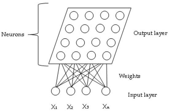
Figure 1.
Structure of a self-organising map.
This model of neural networks learns to group in clusters by using the similarity of the data presented in the inputs, that is, the database used in the training process, even presenting non-linear and high-dimensional characteristics [41]. The pattern of SOM topology entries is defined by Equations (6) and (7) [34]:
where:
- X is the input vector;
- W is the vector of synaptic weights;
- n is the number of entries;
- 1 is the neuron number.
The winning neuron or best matching unit (BMU) is defined by calculating the Euclidean distance, and it is the most used unit with this clustering technique, that is, the neuron that presents the lowest cost or shortest distance, according to Equation (8) [41].
where:
- x is the input vector;
- w is the vector of synaptic weights;
- is the value of the synaptic weight of neuron i;
- n is the number of entries;
- 1 is the neuron number.
Unsupervised training uses the database and iteratively adjusts the synaptic weights to each input sample. The updating of synaptic weights during training is achieved using Equation (9) [49].
where:
- x is the input vector;
- is the value of the synaptic weight of neuron i;
- t is the iteration number;
- is the learning rate defined between 0 and 1;
- describes the neighborhood.
3. Materials and Methods
3.1. Characteristics of the Studied Process
The WTP Alto Cotia has a nominal production capacity of 1.25 m³/s and is located in the metropolitan region of São Paulo. The source of this production system is composed of two dams, known as Cachoeira da Graça and Pedro Beicht. Raw water is captured at the smaller Cachoeira da Graça, and the volume of water is transferred from Pedro Beicht to Cachoeira da Graça using gravity. This WTP has two coagulant dosing application points due to an expansion made to increase the production capacity, which are known as gravity system dosing and pumping system dosing, respectively. Data were collected from SABESP’s laboratory management system for the period ranging from 2010 to 2017, totalling 29,292 records. The data were collected approximately every 2 h during the 12 months, which meant that rainy and dry periods have been contemplated. These data are the result of the ETA operation. Table 1 displays the maximum and minimum values for each physical-chemical parameter.

Table 1.
Maximum and minimum values of physical-chemical parameters.
The physical-chemical parameters that refer to the quality of raw water were the turbidity and colour of the raw water. The efficiency of the coagulation process was measured using the physical-chemical parameters, i.e., the turbidity and colour of the decanted water and the turbidity of the filtered water. The coagulant dosing references were the coagulant dosage system using gravity and the coagulant dosage system using pumping. These variables were considered as outputs, that is, they were the values used in the water treatment process.
3.2. Test Platform and Database
The collected database was submitted to EM and SOM clustering techniques in order to identify scenarios without any preliminary dealings, with the exception of the elimination of outliers. WEKA software [50] version 3.8.6 × 64 was used to process the 29,292 records and 7 attributes related to the process parameters of the WTP under study. The automatic cluster generation option was enabled for this processing, and the heap size increased to 16,394 MB. The study was completed in four parts, as shown in Figure 2 and explained below.
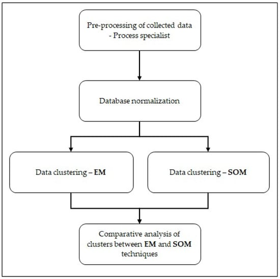
Figure 2.
Steps of the experiments.
- Data pre-processing: manual elimination of values considered inconsistent and null from the raw database (e.g., negative values);
- Normalization of the database with the interval, according to Equation (10);
- Data clustering: use of EM in the pre-processed database;
- Data clustering: use of SOM in the pre-processed database;
- Comparative analysis of the results of the techniques: the analysis and evaluation of clusters generated by EM and SOM in order to identify existing scenarios in the database.
The normalization of attributes was performed according to Equation (10), converting the database to range from 0 to 1 [10].
where:
- is the normalized record value;
- is the record value;
- is the minimum attribute valuer;
- is the maximum attribute value.
Some of the configuration parameters of the EM and SOM techniques were changed as described below, while the others remained with the default values:
EM clustering technique:
- Debug has been changed to true;
- MaxIterations was set to 1000;
- numClusters was set to −1, that is, automatic generation of clusters quantity;
- numKMeansRuns has been changed to 100;
- numExecutionSlots has been changed to 8.
SOM clustering technique:
- calcStats has been changed to true;
- Height and width changed to match the quantity of clusters generated by the EM technique.
The same number of clusters was assigned to make the comparison between the techniques more consistent. The WEKA software used in this work has the option of automatically generating clusters for the EM technique, which obtained 6 clusters between the processing (tests) carried out and were replicated to the tests using the SOM technique. Finally, there is no restriction on the number of clusters for both techniques, that is, the methodology conducted automatic generation using the EM technique, and the number was maintained for subsequent experiments.
4. Results
The processing of the EM algorithm generated six clusters for the database processed with the seven attributes. In this way, the topology using the SOM technique had a height equal to three and width equal to two. The processing time of the EM technique, with the automatic cluster generation option enabled, was 502.94 s, while the SOM technique took 83.8 s. However, when determining the amount of clusters in the EM technique, the time drops to 148.54 s. The results of clustering using the EM and SOM techniques are shown in Table 2 and Table 3, respectively.
Table 2.
Clustering using expectation maximisation.
Table 3.
Clustering using self-organising maps.
The clusters that correspond to the rainy periods were characterized by the highest values of turbidity and colour of the raw water, as well as coagulant dosages. The dry periods were within the clusters with the lowest values of turbidity and raw water colour, as well as the lowest dosage values. The clusters with these intermediate values determine the transition periods, specifically in the autumn and spring seasons.
Table 4 and Table 5 show the results of the EM and SOM processing techniques, respectively, informing the averages of each physical-chemical parameter and coagulant dosage reference. These values show each scenario identified by the techniques used, which have some characteristics that are different among each other.
Table 4.
Clustering using expectation maximisation.
Table 5.
Clustering using self-organising maps.
The EM clustering technique generated three similar scenarios that allowed the identification of different values of physical-chemical parameters of raw water and coagulant dosage. Clusters 0, 1, and 2 represented the lowest values of the turbidity and colour of the raw water and the dosages of the pumping and gravity systems. The biggest difference between these clusters was the colour of the raw water, which had a 15% difference between clusters 0 and 1; the turbidity of the raw water had an approximately 1.5% difference between clusters 0 and 2. The coagulant dosage values had a less than 8% difference between clusters 0 and 1. The next scenario is represented by clusters 3 and 4, which had the values of turbidity and colour of raw water as higher than the first scenario identified. Although the values of turbidity and colour of the raw water remained close, the reference values of the coagulant dosages had a difference of approximately 30%, showing a differential even with the physical-chemical parameters of the raw water, with a differential of less than 5%. The number of classified records for cluster 4 was double compared with cluster 3, showing a longer historical period of the water treatment process. Cluster 4 had lower reference values for coagulant dosages, representing an operational advantage and a possibility of reducing chemical products for the same raw water quality. The third scenario, identified by cluster 5, contained the highest values of the physical-chemical parameters that refer to raw water quality and coagulant dosages. This cluster was characterized by the rainy season, that is, the period with the highest rainfall, resulting in the transfer of the largest amount of suspended materials to the water treatment process.
The SOM clustering technique identified a distinct and additional scenario in relation to the EM clustering technique. Clusters 3 and 5 contained information regarding the dry season scenario, with the lowest values of turbidity and raw water colour. Cluster 3 had turbidity and raw water colour values that were 11.6% and 22.6% lower than cluster 5, respectively. Higher values were also reflected in post-coagulation parameters, such as the colour and turbidity values of the decanted water and the turbidity of the filtered water, in addition to coagulant dosage references. It can be seen that cluster 3 had references for coagulant dosages that were approximately 40% lower, which makes it a favourable cluster with good historical practices for the process.
Clusters 0 and 2 were characterized as another scenario, which have higher raw water turbidity and colour values compared with clusters 3 and 5; consequently, this scenario had higher reference values for the coagulant dosage. Cluster 2 had values of turbidity and colour of raw water that were 3.8% and 1.0% higher than cluster 0, respectively. In this scenario, the values of the colour and turbidity of the decanted water in cluster 2 were 10.7% and 28.5% lower than in cluster 0, respectively, but the dosage values were 3.0% higher. Thus, cluster 0 may be favourable for modelling intelligent models based on process history, as post-coagulation parameters are more adequate and optimized with the operational characteristics of the WTP under study.
Moreover, the coagulant dosage is related to the amount of organic matter and suspended elements present in the raw water. In this way, the destabilization of the electrical charges of the undesirable substances present in the raw water must occur in a way such that the dirt is retained in the subsequent coagulation processes. Increasing the turbidity of the raw water or the colour of the raw water requires the coagulant dosage to be increased so that the turbidity or colour of the settled water is kept within the acceptable limits of the water treatment process. When the turbidity and colour values of the raw water decrease, the dosage references must be reduced so that the process remains within operational limits without wasting chemical products unnecessarily.
The SOM clustering technique identified two distinct scenarios in relation to the EM clustering technique. The references of the turbidity and colour of raw water were the highest, characterizing rainy periods; in other words, cluster 4 showed an intermediate scenario and cluster 1 had the highest values of turbidity and colour of raw water. The differentials were 23.1% and 37.1%, respectively, in relation to raw water quality, whereas the dosages had reference values greater than 30%.
However, the SOM clustering technique identified two scenarios with higher values for raw water parameters (clusters 1 and 4), whereas the EM clustering technique identified a scenario with the lowest values of raw water parameters (cluster 0), characterizing a scenario of a period of little rain or drought. In this way, the techniques showed a distinction in relation to the historical data. That is, the EM showed that a quantity of data can be highlighted because the cluster 0 data do not show more optimized values in relation to the other identified scenarios, while the SOM identified a favourable scenario to be considered for the rainy season, i.e., the data selected by cluster 4, as the coagulant dosage references were reduced in relation to cluster 1.
Figure 3 and Figure 4 show the physical-chemical parameters and coagulant dosage references of each cluster, showing the dispersion contained in each cluster through the boxplots. This information provides the details of the groups of techniques that are presented in a consolidated form in Table 2 and Table 3, which refer to the EM and SOM techniques, respectively.
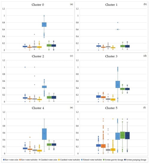
Figure 3.
Boxplot graph (EM).
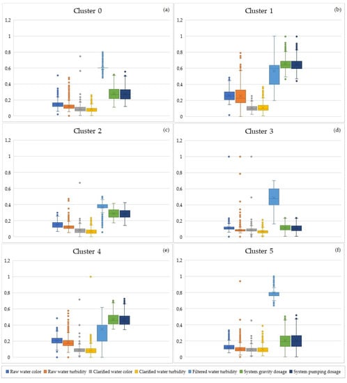
Figure 4.
Boxplot graph (SOM).
Figure 3a shows the results of cluster 0 with the physical-chemical parameters relating to the raw water quality with the lowest interquartile dispersion in relation to the other clusters. The results show that there were outliers in all parameters, with most being concentrated in the parameters of the colour and turbidity of the decanted water and the turbidity of the filtered water. The dispersion of the filtered water parameter was the highest among the scenarios that had low raw water colour and turbidity values. The other parameters, post-coagulation and dosages, also showed greater dispersion in relation to clusters 1 and 2.
Figure 3b shows the result of cluster 1, highlighting the behaviour of the turbidity parameter of the filtered water, which had a value fixed at 0.4 NTU and presented an outlier after the upper limit. The physical-chemical parameters and dosages had the lowest dispersions in relation to clusters 0 and 2; however, this characteristic did not extend to the parameters of the colour and turbidity of the raw water.
Figure 3c shows the result of cluster 2, highlighting that the coagulant dosages do not have outliers. In addition, the physical-chemical parameters of the colour of raw and decanted water have the most distant outliers in relation to the maximum limit. The dispersion of raw water colour was equal to that of cluster 0, but smaller compared with cluster 1. The scenario with the closest results to cluster 2 was cluster 1. With the exception of raw water colour, the other cluster parameters in cluster 2 have larger dispersions compared with cluster 1.
Figure 3d shows the result of cluster 3, which had higher raw water colour and turbidity values compared with cluster 0 to 2; that is, it was characterized by the highest rainfall in this grouping. All parameters had outliers; however, the turbidity of the filtered water contained the most points beyond the lower and upper limits.
Figure 3e shows the result of cluster 4, which had a scenario similar to the scenario of cluster 3. The main differences were the smaller dispersions of raw water parameters and the colour and turbidity of the decanted water. The parameters of the turbidity of the filtered water and dosages had greater dispersions in relation to cluster 3. It can be observed that the turbidity of the filtered water did not have outliers; however, it had the greatest dispersion among the other clusters obtained after using the EM technique.
Figure 3f shows the scenario in relation to the highest rainfall index, that is, the scenario with the highest values of colour and turbidity of raw water and, consequently, the highest values of coagulant dosages. It can be seen that cluster 5 had the highest dispersions in all parameters, in addition to the existence of outliers in all parameters, when focusing on the turbidity parameters of the raw and decanted water. The possible reason for having only one scenario representing the rainy season is the reduced amount of data, as these situations occur less frequently in the water treatment process.
Table 6 shows the minimum, maximum, first and third quartiles, mean, median, and interquartile range values of the parameters of each cluster resulting from the application of the EM technique. Through Figure 3a–f and Table 6, it can be seen that clusters 2, 4, and 5 are appropriate to be selected for training intelligent models for predicting coagulant dosage based on the history of the water treatment process. The exclusion of outliers from these clusters is mandatory in order to avoid scenarios that could compromise the learning of the computational model.
Table 6.
Boxplot values of the parameters and cluster of the EM technique.
Figure 4a shows the result referring to cluster 0 of the SOM technique. This scenario presented an intermediate rainfall index and was similar to cluster 2. The raw water colour and turbidity values were higher in relation to clusters 3 and 5, which showed scenarios with better raw water quality; that is, cluster 0 is characterized as the dry season.
The filtered water parameter behaved similarly to cluster 1 of the EM technique, keeping the value fixed at 0.4 NTU. Another difference was found in the values of raw water parameters, which differed between the EM and SOM techniques, that is, the SOM technique resulted in higher values.
Figure 4b presents cluster 1, which is characterized as the scenario with the highest rainfall, showing the rainy season of the database that was submitted to processing. It is observed that the turbidity of the filtered water did not have outliers; however the other parameters did. The dispersion of the turbidity of the filtered water was the greatest in relation to the other clusters, which may be caused by the low amount of data that related to the rainy season. In the same way as cluster 0, the colour and turbidity of the decanted water did not have outliers at the lower limit.
Figure 4c shows cluster 2, which represented the intermediate scenario and was similar to that presented in cluster 0. With the exception of the turbidity of the filtered water, the other parameters did not show outliers at the lower limit. The raw water parameters were close, as well as the coagulant dosage values; however, they significantly differ.
The colour dispersions of the raw water and the turbidity of the decanted water were higher in relation to cluster 0. The other parameters had smaller dispersions, with the exception of the turbidity of the filtered water in cluster 0, which had a value of 0.
Figure 4d is related to the scenario with the best quality of raw water, that is, the scenario with the lowest values of colour and turbidity of raw water. A similar scenario was found in cluster 5. The turbidity parameter of the filtered water had no outlier, unlike the other parameters. The coagulant dosages had only one reference that was considered as an outlier in consideration that little information could be discarded.
The colour and turbidity of the raw water and the colour of the decanted water had several outliers far from the upper limit, whereas the turbidity outliers of the decanted water were close to the upper limit, which shows the importance of this resource for the evaluation of clustering.
Figure 4e shows a scenario not identified by the EM technique that was classified within a rainy period, but with lower rainfall rates. The coagulant dosage values and raw water parameters were lower compared with cluster 1; four different scenarios were identified with the SOM technique, while the EM technique identified three.
It can be considered that this scenario was merged with the rainy season scenario in the EM technique; however, cluster 4 allows for the exploration of an intermediate scenario, which increases the complexity from an operational point of view. The parameters had outliers with the exception of the turbidity of the filtered water, showing that undesired data always occur in all clusters.
Figure 4f shows cluster 5, which represented a scenario similar to that presented in cluster 3. However, cluster 5 presented values for colour and turbidity of raw water and coagulant dosages that were higher than cluster 3.
The dispersions of colour and turbidity of the raw water, colour and turbidity of the decanted water, and coagulant dosages were also superior in relation to cluster 3, only maintaining the turbidity of the filtered water with less dispersion.
Table 7 shows the minimum, maximum, first and third quartile values, mean, median, and interquartile range of the parameters of each cluster resulting from the application of the SOM technique. By observing Figure 4a–f and Table 7, it is verified that clusters 0, 1, 3, and 4 are appropriate to be selected for training intelligent models for predicting coagulant dosage based on historical water treatment process. As with the EM technique, the exclusion of outliers from these clusters were also mandatory.
Table 7.
Boxplot values of the parameters and cluster of the SOM.
5. Discussion
The coagulation process is characterized as a non-linear and multi-parameter step when considering raw water parameters. The values of the turbidity and colour of raw water vary according to the rainy and dry season with respect to the highest and lowest values, respectively. The coagulant dosage should consider these changes, not in a linear way, but according to historical tests or jar tests to determine the most adequate dosage for the present scenario. In addition, the post-coagulation parameters must also be considered with the aim of optimizing the dosages because for the same value of turbidity and colour of raw water, the dosage values can change depending on the efficiency of the coagulation and flocculation. In this way, the parameters of the decantation and filtration steps may be relevant for decision making for a possible reduction or increase in coagulant dosages when the raw water quality remains stable.
The EM and SOM clustering techniques have been applied in several studies in the area of water resources to identify operational scenarios or unforeseen conditions. However, specifically, no reference was found that used the EM technique in the selection of data for the construction of intelligent models for the prediction of coagulant dosage references. This limitation forced the comparison to be made with other studies that focused on water resources, which obtained satisfactory results with the application of both techniques.
In [38], the SOM technique resulted in five different scenarios of a water treatment plant, covering the most common scenarios and the situations that did not require greater attention in order to avoid damage to the process. It can be observed that the identification of scenarios allows for a more accurate decision-making process in relation to possible operational conditions.
According to [30], the EM technique enabled the identification of scenarios of 21 sites through the examination of physical-chemical parameters in relation to the water quality of the hydrographic basins. The results show that five clusters were used to identify the classes.
In this study, we used six clusters to classify the historical database and focused on the coagulation process of a water treatment plant. The number of clusters was determined by the EM technique itself and the WEKA data mining tool; from then on, the number was replicated using the SOM technique. The number of clusters was smaller by one; however, the database used in the proposed study is 7 years old and has approximately 29,300 records, which may be a possible reason for the greater number of clusters.
Another important point to be observed is the use of physical-chemical parameters that were submitted to clustering processes with the common purpose of identifying or classifying operational scenarios, which helps during decision making or data selection for intelligent models that use algorithms of supervised training.
The results of the EM and SOM techniques showed that a database can provide different scenarios of water quality and operational practices. The EM technique presented scenarios with lower raw water colour and turbidity values compared with the SOM technique, showing that the results must be carefully evaluated and aimed at choosing the most appropriate data possible. An important point in both techniques was the low dispersion of the turbidity parameter of the filtered water, with the other parameters showing different values. In this way, it can be considered that the techniques identified the pattern in the turbidity of the filtered water, but in different scenarios.
The clusters with the smallest dispersions show that the technique identified scenarios with less variation in the parameters related to raw water quality, such as turbidity and colour, which can be considered an adequate selection of data for later use in training intelligent models. The clusters with smaller dispersions can be considered as good options.
In the boxplot graphs, it was possible to identify the outliers that should be discarded if the respective scenarios were considered for later stages of model construction, such as the modelling of intelligent systems based on supervised training. Although both techniques can be used alone or in combination, the EM technique resulted in a smaller number of scenarios compared with the SOM technique, which can lead to more efficient systems.
6. Conclusions
This study addressed the use of two clustering techniques to identify quality scenarios and operational practices in a water treatment plant, which was performed to select data for training intelligent models for predicting coagulant reference dosages with the aim of obtaining economic, social, and environmental gains.
The results showed that both techniques are viable for the purpose; however, the EM technique identified a lower number of scenarios, which is considered to be preferable for modelling using algorithms that use supervised training.
The clustering techniques used have different processing and convergence contexts, as can be seen in the theoretical framework. The results show that some differences were proposed by both and can facilitate the evaluation and decision making of data selection processes. The difference that can be highlighted is the intermediate scenario of the SOM technique, which represents a specific rainy season but with lower rainfall rates, as the raw water quality parameters were not the highest in relation to all clusters. Another important point that can be highlighted is the lack of the use of the EM technique to perform clustering for data selection for training intelligent models, as proposed in this study. In this way, the EM technique proves to be viable for this purpose, as well as in the classification of scenarios in the field of water resources.
Moreover, the good operational practices identified in the evaluated clusters can bring benefits to the process, such as a reduction of expenses using chemical products, specifically for the coagulant, which requires the extraction from nature to be manufactured for later use in the water treatment process; in addition, more benefits can be gained by significantly reducing the generation of waste that is sent for a final destination at wastewater treatment plants or sludge treatment facilities, as such waste cannot be discharged into the environment, thus reducing environmental problems.
Author Contributions
Conceptualisation, A.F.H.L. and F.C.R.d.S.; methodology, A.F.H.L. and F.C.R.d.S.; software, F.C.R.d.S.; validation, A.F.H.L. and F.C.R.d.S.; formal analysis, A.F.H.L. and F.C.R.d.S.; investigation, A.F.H.L. and F.C.R.d.S.; resources, A.F.H.L. and F.C.R.d.S.; data curation, F.C.R.d.S.; writing—original draft preparation, A.F.H.L. and F.C.R.d.S.; writing—review and editing, A.F.H.L. and F.C.R.d.S.; visualisation, A.F.H.L. and F.C.R.d.S.; supervision, A.F.H.L.; project administration, A.F.H.L. All authors have read and agreed to the published version of the manuscript.
Funding
This research received no external funding.
Institutional Review Board Statement
Not applicable.
Informed Consent Statement
Not applicable.
Data Availability Statement
All data are contained in the article.
Acknowledgments
The authors would like to thank the Universidade Nove de Julho—UNINOVE for supporting this work.
Conflicts of Interest
The authors declare no conflict of interest.
Abbreviations
The following abbreviations are used in this manuscript:
| ANN | Artificial neural networks |
| MDPI | Multidisciplinary Digital Publishing Institute |
| mg/L | Milligrams per litre |
| MLP | Multilayer perceptron |
| m/s | Cubic metre per second |
| NTU | Nephelometric turbidity unit |
| EM | Expectation maximisation |
| SOM | Self-organising maps |
| PCA | Principal component analysis |
| Probability density function | |
| Pt-Co | Platinum-Cobalt scale |
| WTP | Water treatment plants |
| WWTP | Wastewater treatment plants |
References
- Gomes, M.G.; da Silva, V.H.C.; Pinto, L.F.R.; Centoamore, P.; Digiesi, S.; Facchini, F.; Neto, G.C.d.O. Economic, Environmental and Social Gains of the Implementation of Artificial Intelligence at Dam Operations toward Industry 4.0 Principles. Sustainability 2020, 12, 3604. [Google Scholar] [CrossRef]
- O’Reilly, G.; Bezuidenhout, C.C.; Bezuidenhout, J.J. Artificial neural networks: Applications in the drinking water sector. Water Supply 2018, 18, 1869–1887. [Google Scholar] [CrossRef]
- Olanweraju, R.F.; Muyibi, S.A.; Salawudeen, T.O.; Aibinu, A.M. An intelligent modeling of coagulant dosing system for water treatment plants based on artificial neural network. Aust. J. Basic Appl. Sci. 2012, 6, 93–99. [Google Scholar]
- Fkirin, M.A.; Zedan, R. Identification of water treatment plant based on feedforward neural network. Control Cybern. 2017, 46, 247–258. [Google Scholar]
- Librantz, A.F.; dos Santos, F.C.R.; Dias, C.G. Artificial neural networks to control chlorine dosing in a water treatment plant. Acta Scientiarum. Technol. 2018, 40, 37275. [Google Scholar] [CrossRef]
- Naceradska, J.; Pivokonska, L.; Pivokonsky, M. On the importance of pH value in coagulation. J. Water Supply Res. Technol.-Aqua 2019, 68, 222–230. [Google Scholar] [CrossRef]
- Lamrini, B.; Lakhal, E.K.; Lann, M.V.L. A decision support tool for technical processes optimization in drinking water treatment. Desalin. Water Treat. 2013, 52, 4079–4088. [Google Scholar] [CrossRef]
- Gamiz, J.; Vilanova, R.; Martinez-Garcia, H.; Bolea, Y.; Grau, A. Fuzzy Gain Scheduling and Feed-Forward Control for Drinking Water Treatment Plants (DWTP) Chlorination Process. IEEE Access 2020, 8, 110018–110032. [Google Scholar] [CrossRef]
- Leite, R.; Amorim, M.; Rodrigues, M.; Oliveira Neto, G. Overcoming Barriers for Adopting Cleaner Production: A Case Study in Brazilian Small Metal-Mechanic Companies. Sustainability 2019, 11, 4808. [Google Scholar] [CrossRef]
- Bobadilla, M.C.; Lorza, R.; García, R.E.; Gómez, F.S.; González, E.V. Coagulation: Determination of Key Operating Parameters by Multi-Response Surface Methodology Using Desirability Functions. Water 2019, 11, 398. [Google Scholar] [CrossRef]
- Lin, J.L.; Ika, A.R. Enhanced Coagulation of Low Turbid Water for Drinking Water Treatment: Dosing Approach on Floc Formation and Residuals Minimization. Environ. Eng. Sci. 2019, 36, 732–738. [Google Scholar] [CrossRef]
- Liu, W.; Ratnaweera, H. Improvement of multi-parameter-based feed-forward coagulant dosing control systems with feed-back functionalities. Water Sci. Technol. 2016, 74, 491–499. [Google Scholar] [CrossRef]
- Heddam, S.; Dechemi, N. A new approach based on the dynamic evolving neural-fuzzy inference system (DENFIS) for modelling coagulant dosage (Dos): Case study of water treatment plant of Algeria. Desalin. Water Treat. 2015, 53, 1045–1053. [Google Scholar] [CrossRef]
- Ratnaweera, H.; Fettig, J. State of the Art of Online Monitoring and Control of the Coagulation Process. Water 2015, 7, 6574–6597. [Google Scholar] [CrossRef]
- Wang, K.J.; Wang, P.S.; Nguyen, H.P. A data-driven optimization model for coagulant dosage decision in industrial wastewater treatment. Comput. Chem. Eng. 2021, 152, 107383. [Google Scholar] [CrossRef]
- Jayaweera, C.D.; Aziz, N. An efficient neural network model for aiding the coagulation process of water treatment plants. Environ. Dev. Sustain. 2021, 24, 1069–1085. [Google Scholar] [CrossRef]
- Liu, Y.; He, Y.; Li, S.; Dong, Z.; Zhang, J.; Kruger, U. An Auto-Adjustable and Time-Consistent Model for Determining Coagulant Dosage Based on Operators’ Experience. IEEE Trans. Syst. Man Cybern. Syst. 2021, 51, 5614–5625. [Google Scholar] [CrossRef]
- Maleki, A.; Nasseri, S.; Aminabad, M.S.; Hadi, M. Comparison of ARIMA and NNAR Models for Forecasting Water Treatment Plant’s Influent Characteristics. KSCE J. Civ. Eng. 2018, 22, 3233–3245. [Google Scholar] [CrossRef]
- Menkiti, M.C.; Ejimofor, M.I. Experimental and artificial neural network application on the optimization of paint effluent (PE) coagulation using novel Achatinoidea shell extract (ASE). J. Water Process Eng. 2016, 10, 172–187. [Google Scholar] [CrossRef]
- Al-Adhaileh, M.H.; Alsaade, F.W. Modelling and Prediction of Water Quality by Using Artificial Intelligence. Sustainability 2021, 13, 4259. [Google Scholar] [CrossRef]
- dos Santos, F.C.R.; Librantz, A.F.H.; Dias, C.G.; Rodrigues, S.G. Intelligent system for improving dosage control. Acta Scientiarum. Technol. 2017, 39, 33. [Google Scholar] [CrossRef]
- Wadkar, D.V.; Karale, R.S.; Wagh, M.P. Application of cascade feed forward neural network to predict coagulant dose. J. Appl. Water Eng. Res. 2021, 1–14. [Google Scholar] [CrossRef]
- Liu, W.; Ratnaweera, H.; Kvaal, K. Model-based measurement error detection of a coagulant dosage control system. Int. J. Environ. Sci. Technol. 2018, 16, 3135–3144. [Google Scholar] [CrossRef]
- Castillo, E.; Corrales, D.C.; Lasso, E.; Ledezma, A.; Corrales, J.C. Water quality detection based on a data mining process on the California estuary. Int. J. Bus. Intell. Data Min. 2017, 12, 406. [Google Scholar] [CrossRef]
- Hadi, S.J.; Abba, S.I.; Sammen, S.S.; Salih, S.Q.; Al-Ansari, N.; Yaseen, Z.M. Non-Linear Input Variable Selection Approach Integrated with Non-Tuned Data Intelligence Model for Streamflow Pattern Simulation. IEEE Access 2019, 7, 141533–141548. [Google Scholar] [CrossRef]
- Faraj, F.; Shen, H. Forecasting the Environmental Parameters of Water Resources Using Machine Learning Methods. Ann. Adv. Agric. Sci. 2018, 2. [Google Scholar] [CrossRef]
- Onyutha, C.; Kwio-Tamale, J.C. Modelling chlorine residuals in drinking water: A review. Int. J. Environ. Sci. Technol. 2022, 19, 11613–11630. [Google Scholar] [CrossRef]
- Bui, H.; Duong, H.; Nguyen, C. Applying an Artificial Neural Network to Predict Coagulation Capacity of Reactive Dyeing Wastewater by Chitosan. Pol. J. Environ. Stud. 2016, 25, 545–555. [Google Scholar] [CrossRef]
- dos Santos, F.C.R.; Librantz, A.F.H.; Sassi, R.J. An Approach to Clustering Using the Expectation-Maximization and Selection of Attributes ReliefF Applied to Water Treatment Plants process. In Proceedings of the Progress in Pattern Recognition, Image Analysis, Computer Vision, and Applications; Mendoza, M., Velastín, S., Eds.; Springer International Publishing: Cham, Switzerland, 2018; pp. 558–565. [Google Scholar]
- Di, Z.; Chang, M.; Guo, P. Water Quality Evaluation of the Yangtze River in China Using Machine Learning Techniques and Data Monitoring on Different Time Scales. Water 2019, 11, 339. [Google Scholar] [CrossRef]
- Fahimi, F.; Yaseen, Z.M.; El-shafie, A. Application of soft computing based hybrid models in hydrological variables modeling: A comprehensive review. Theor. Appl. Climatol. 2016, 128, 875–903. [Google Scholar] [CrossRef]
- Chen, Y.; Song, L.; Liu, Y.; Yang, L.; Li, D. A Review of the Artificial Neural Network Models for Water Quality Prediction. Appl. Sci. 2020, 10, 5776. [Google Scholar] [CrossRef]
- Zhao, L.; Dai, T.; Qiao, Z.; Sun, P.; Hao, J.; Yang, Y. Application of artificial intelligence to wastewater treatment: A bibliometric analysis and systematic review of technology, economy, management, and wastewater reuse. Process Saf. Environ. Prot. 2020, 133, 169–182. [Google Scholar] [CrossRef]
- Chang, K.; Gao, J.L.; Wu, W.Y.; Yuan, Y.X. Water quality comprehensive evaluation method for large water distribution network based on clustering analysis. J. Hydroinform. 2011, 13, 390–400. [Google Scholar] [CrossRef]
- Astel, A.; Tsakovski, S.; Barbieri, P.; Simeonov, V. Comparison of self-organizing maps classification approach with cluster and principal components analysis for large environmental data sets. Water Res. 2007, 41, 4566–4578. [Google Scholar] [CrossRef]
- Bieroza, M.; Baker, A.; Bridgeman, J. New data mining and calibration approaches to the assessment of water treatment efficiency. Adv. Eng. Softw. 2012, 44, 126–135. [Google Scholar] [CrossRef]
- Haghiri, S.; Daghighi, A.; Moharramzadeh, S. Optimum coagulant forecasting by modeling jar test experiments using ANNs. Drink. Water Eng. Sci. 2018, 11, 1–8. [Google Scholar] [CrossRef]
- Juntunen, P.; Liukkonen, M.; Lehtola, M.; Hiltunen, Y. Cluster analysis by self-organizing maps: An application to the modelling of water quality in a treatment process. Appl. Soft Comput. 2013, 13, 3191–3196. [Google Scholar] [CrossRef]
- Olawoyin, R.; Nieto, A.; Grayson, R.L.; Hardisty, F.; Oyewole, S. Application of artificial neural network (ANN)–self-organizing map (SOM) for the categorization of water, soil and sediment quality in petrochemical regions. Expert Syst. Appl. 2013, 40, 3634–3648. [Google Scholar] [CrossRef]
- Kalteh, A.; Hjorth, P.; Berndtsson, R. Review of the self-organizing map (SOM) approach in water resources: Analysis, modelling and application. Environ. Model. Softw. 2008, 23, 835–845. [Google Scholar] [CrossRef]
- Nourani, V.; Baghanam, A.H.; Adamowski, J.; Gebremichael, M. Using self-organizing maps and wavelet transforms for space–time pre-processing of satellite precipitation and runoff data in neural network based rainfall–runoff modeling. J. Hydrol. 2013, 476, 228–243. [Google Scholar] [CrossRef]
- Borzooei, S.; Miranda, G.H.B.; Abolfathi, S.; Scibilia, G.; Meucci, L.; Zanetti, M.C. Application of unsupervised learning and process simulation for energy optimization of a WWTP under various weather conditions. Water Sci. Technol. 2020, 81, 1541–1551. [Google Scholar] [CrossRef]
- Keshavarz, M.; Huang, B. Expectation Maximization method for multivariate change point detection in presence of unknown and changing covariance. Comput. Chem. Eng. 2014, 69, 128–146. [Google Scholar] [CrossRef]
- Dempster, A.P.; Laird, N.M.; Rubin, D.B. Maximum Likelihood from Incomplete Data via the EM Algorithm. J. R. Stat. Soc. Ser. B 1977, 39, 1–38. [Google Scholar]
- North, B.; Blake, A. Using expectation-maximisation to learn dynamical models from visual data. Image Vis. Comput. 1999, 17, 611–616. [Google Scholar] [CrossRef]
- McLachlan, G.J.; Krishnan, T. The EM Algorithm and Extensions, 2nd ed.; John Wiley & Sons, Inc.: Hoboken, NJ, USA, 2008. [Google Scholar]
- Witten, I.H.; Eibe Frank, M.A.H.; Pal, C.J. Data Mining: Practical Machine Learning Tools and Techniques, 4th ed.; Elsevier: Amsterdam, The Netherlands, 2017. [Google Scholar] [CrossRef]
- Kohonen, T. The self-organizing map. Proc. IEEE 1990, 78, 1464–1480. [Google Scholar] [CrossRef]
- Lamrini, B.; Lakhal, E.K.; Lann, M.V.L.; Wehenkel, L. Data validation and missing data reconstruction using self-organizing map for water treatment. Neural Comput. Appl. 2011, 20, 575–588. [Google Scholar] [CrossRef]
- Hall, M.; Frank, E.; Holmes, G.; Pfahringer, B.; Reutemann, P.; Witten, I.H. The WEKA data mining software: An update. SIGKDD Explor. Newsl. 2009, 11, 10–18. [Google Scholar] [CrossRef]


Disclaimer/Publisher’s Note: The statements, opinions and data contained in all publications are solely those of the individual author(s) and contributor(s) and not of MDPI and/or the editor(s). MDPI and/or the editor(s) disclaim responsibility for any injury to people or property resulting from any ideas, methods, instructions or products referred to in the content. |
© 2023 by the authors. Licensee MDPI, Basel, Switzerland. This article is an open access article distributed under the terms and conditions of the Creative Commons Attribution (CC BY) license (https://creativecommons.org/licenses/by/4.0/).