
Model-Based Reinforcement Learning Method for Microgrid Optimization Scheduling


Abstract
:1. Introduction
- This study converts the microgrid optimization scheduling issue into reinforcement learning tasks by identifying the observation space, state space, and reward functions within the microgrid model.
- This paper introduces model-based reinforcement learning to address the optimal scheduling problem in microgrid systems, which adopts the MuZero algorithm’s excellent performance in discrete action spaces into the application of Monte Carlo Tree Search for the determination of the optimal strategy.
- This paper builds a joint training model for three major networks to enable the algorithm to learn and optimize simultaneously for environmental dynamic and optimal strategy determination without prior professional knowledge.
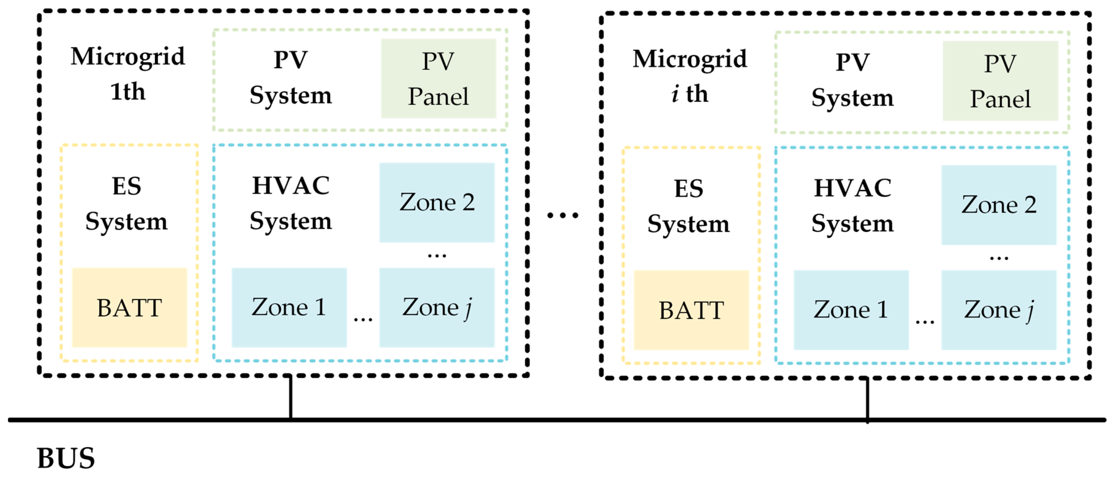
2. Microgrid Scheduling Model
2.1. HVAC System
2.1.1. Discomfort Reward
2.1.2. Energy Consumption Reward
2.1.3. HVAC System Reward
2.2. PV System
2.3. ES System
2.4. System Reward
2.5. Model Reward
3. Algorithm Design
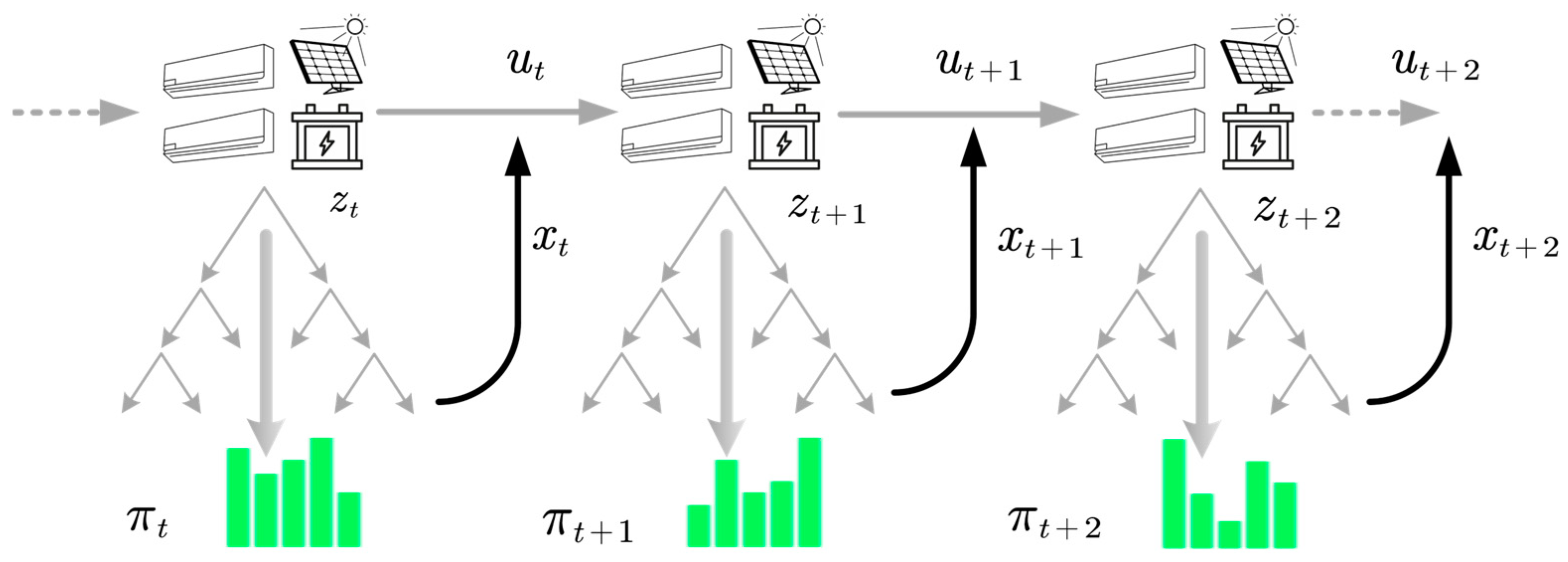
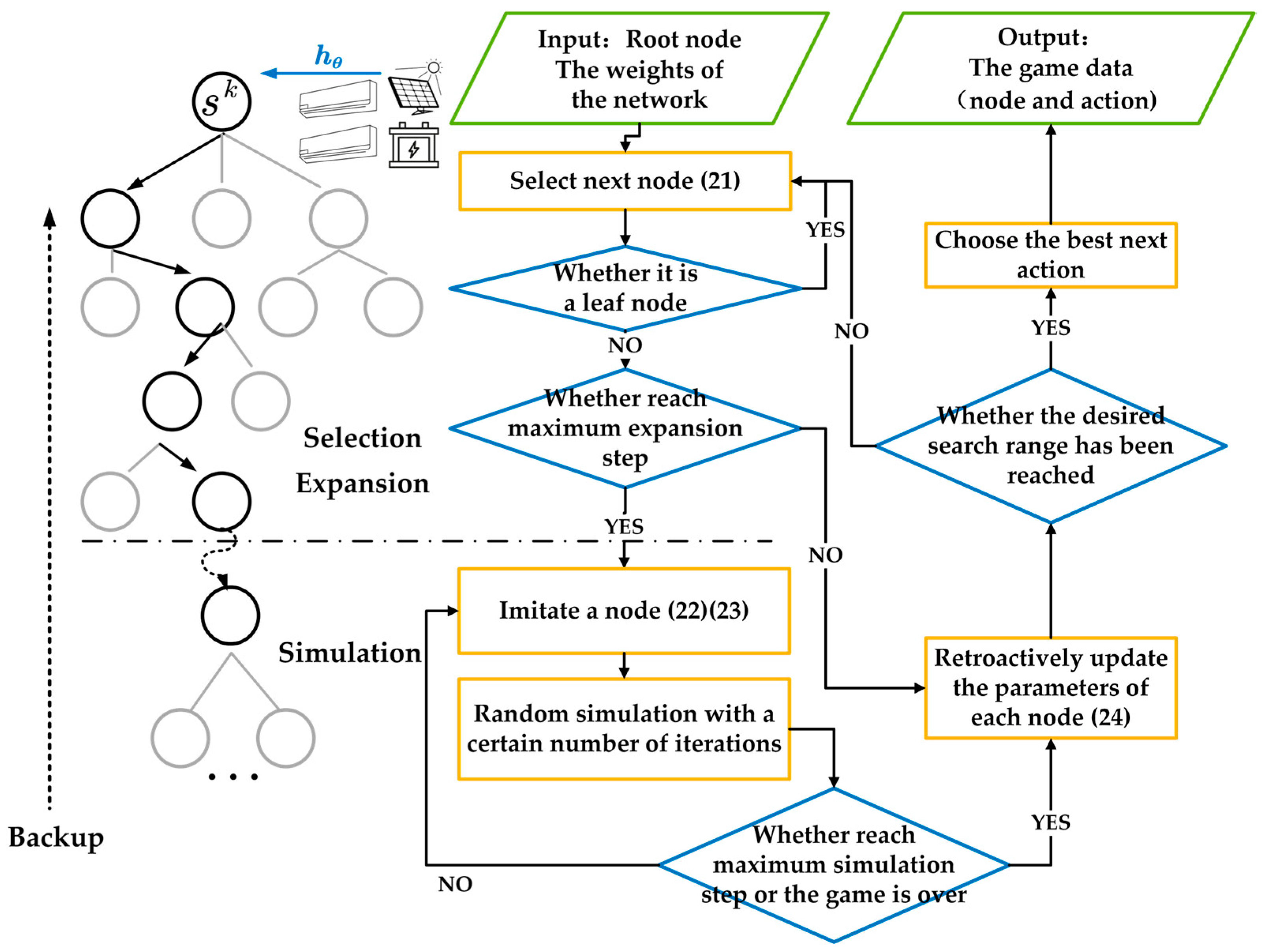
3.1. Self-Play
3.1.1. Selection
3.1.2. Expansion
3.1.3. Backup
3.2. Trainer
3.2.1. Representation Function
3.2.2. Prediction Function
3.2.3. Dynamic Function
3.2.4. Training Process
| Algorithm 1: The Pseudocode of Trainer |
| Input: Game data from the self-play process, the current parameters of the Representation, Prediction and Dynamic model. Output: The updated weight parameters of the model. 1 start 2 (25) representation function to transform the observation into hiden state 3 repeat 4 (26) prediction function to choose the action and estimate the value 5 (27) dynamic function to use the environmental dynamics and reward function to calculate the next state and corresponding reward 6 (28) to update 7 until complete a game training batch 4 end |
4. Simulation Results
4.1. Model and Neural Network Parameter Design
4.1.1. Microgrid Scheduling Model Parameters
4.1.2. Reinforcement Learning Algorithm Parameters
4.1.3. Neural Network Parameters
4.2. Result
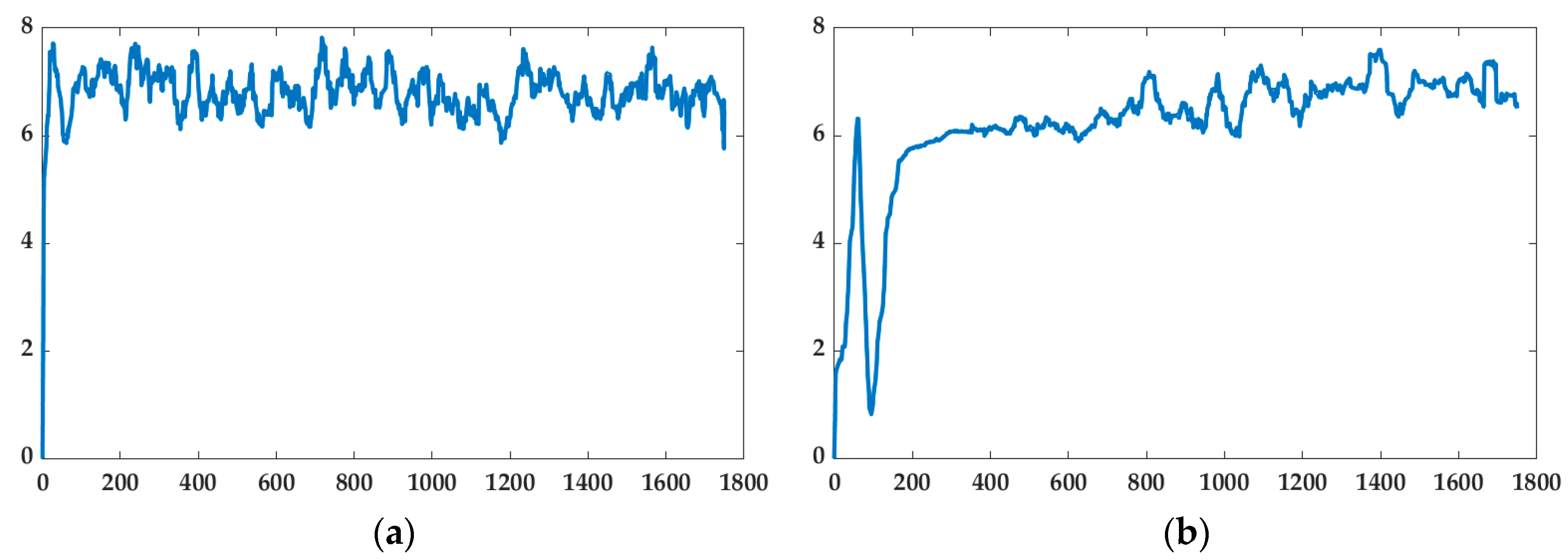
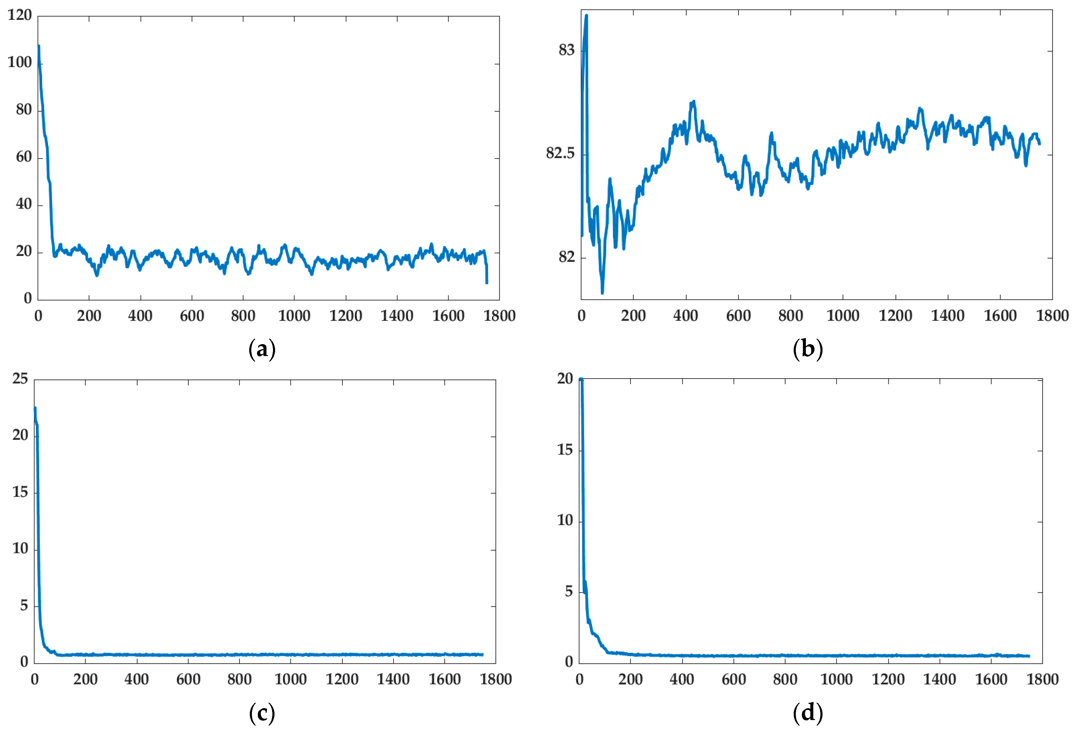
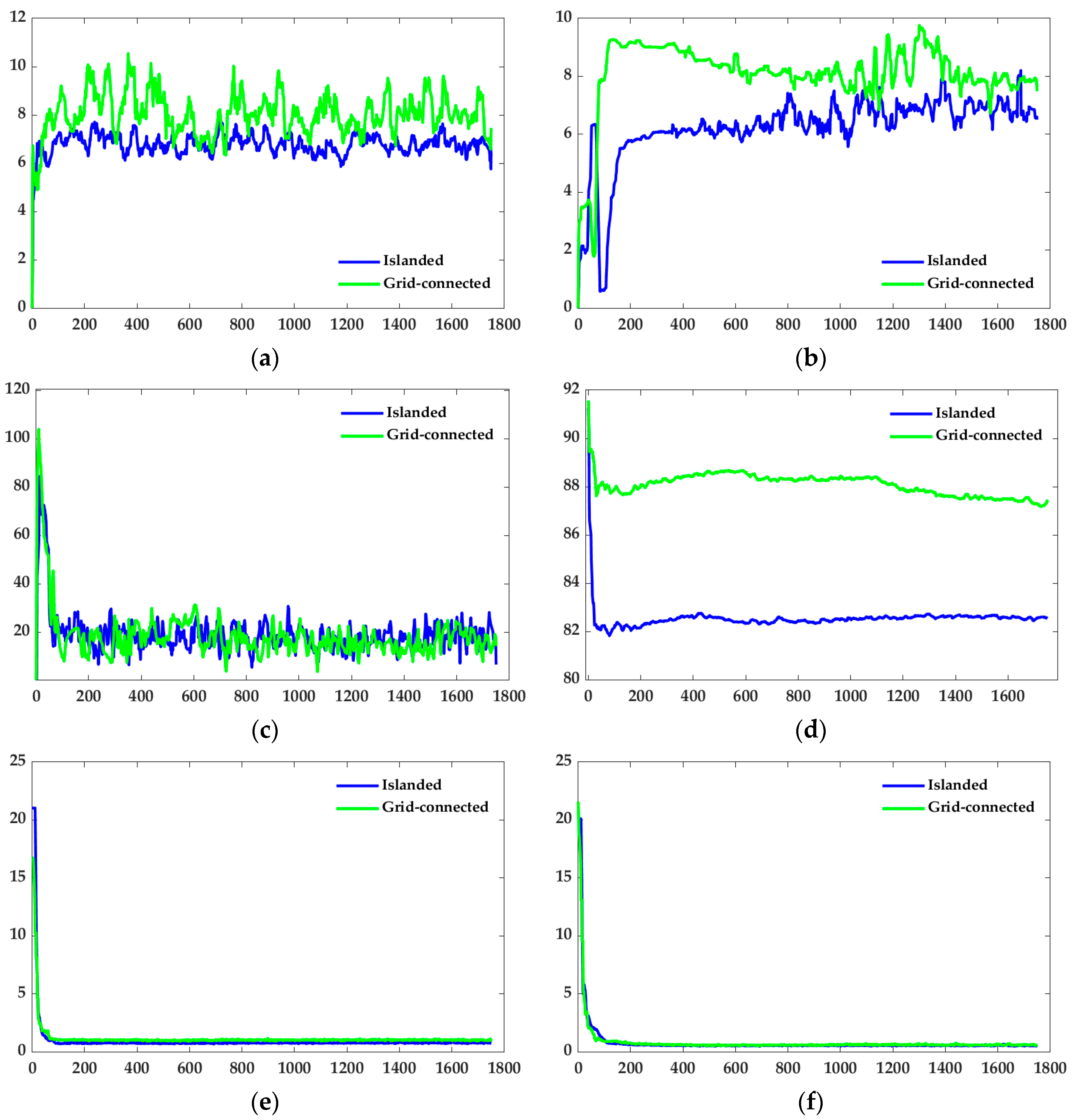
4.2.1. Islanded Operation
4.2.2. Grid-Connected Operation
5. Conclusions
Author Contributions
Funding
Data Availability Statement
Conflicts of Interest
References
- Alanne, K.; Saari, A. Distributed energy generation and sustainable development. Renew. Sustain. Energy Rev. 2006, 10, 539–558. [Google Scholar] [CrossRef]
- Song, Z.; Wang, X.; Wei, B.; Shan, Z.; Guan, P. Distributed Finite-Time Cooperative Economic Dispatch Strategy for Smart Grid under DOS Attack. Mathematics 2023, 11, 2103. [Google Scholar] [CrossRef]
- Li, Y.; Gao, D.W.; Gao, W.; Zhang, H.; Zhou, J. A Distributed Double-Newton Descent Algorithm for Cooperative Energy Management of Multiple Energy Bodies in Energy Internet. IEEE Trans. Ind. Inform. 2021, 17, 5993–6003. [Google Scholar] [CrossRef]
- Zhang, H.; Li, Y.; Gao, D.W.; Zhou, J. Distributed Optimal Energy Management for Energy Internet. IEEE Trans. Ind. Inform. 2017, 13, 3081–3097. [Google Scholar] [CrossRef]
- Parhizi, S.; Lotfi, H.; Khodaei, A.; Bahramirad, S. State of the art in research on microgrids: A review. IEEE Access 2015, 3, 890–925. [Google Scholar] [CrossRef]
- Li, T.; Huang, R.; Chen, L.; Jensen, C.S.; Pedersen, T.B. Compression of Uncertain Trajectories in Road Networks. In Proceedings of the 46th International Conference on Very Large Data Bases, Online, 31 August–4 September 2020; Volume 13, pp. 1050–1063. [Google Scholar]
- Rezvani, A.; Gandomkar, M.; Izadbakhsh, M.; Ahmadi, A. Environmental/economic scheduling of a micro-grid with renewable energy resources. J. Clean. Prod. 2015, 87, 216–226. [Google Scholar] [CrossRef]
- Li, Y.; Zhang, H.; Liang, X.; Huang, B. Event-triggered based distributed cooperative energy management for multienergy systems. IEEE Trans. Ind. Inf. 2019, 15, 2008–2022. [Google Scholar] [CrossRef]
- Liu, C.; Wang, D.; Yin, Y. Two-Stage Optimal Economic Scheduling for Commercial Building Multi-Energy System through Internet of Things. IEEE Access 2019, 7, 174562–174572. [Google Scholar] [CrossRef]
- Li, Y.; Gao, D.W.; Gao, W.; Zhang, H.; Zhou, J. Double-Mode Energy Management for Multi-Energy System via Distributed Dynamic Event-Triggered Newton-Raphson Algorithm. IEEE Trans. Smart Grid 2020, 11, 5339–5356. [Google Scholar] [CrossRef]
- Eseye, A.T.; Zheng, D.; Zhang, J.; Wei, D. Optimal energy management strategy for an isolated industrial microgrid using a modified particle swarm optimization. In Proceedings of the 2016 IEEE International Conference on Power and Renewable Energy (ICPRE), Shanghai, China, 21–23 October 2016; pp. 494–498. [Google Scholar]
- Zeng, Y.; Zhao, H.; Liu, C.; Chen, S.; Hao, X.; Sun, X.; Zhang, J. Multi objective optimization of microgrid based on Improved Multi-objective Particle Swarm Optimization. In Proceedings of the 2022 International Seminar on Computer Science and Engineering Technology (SCSET), Indianapolis, IN, USA, 8–9 January 2022; pp. 80–83. [Google Scholar]
- Elsayed, W.T.; Hegazy, Y.G.; Bendary, F.M.; El-Bages, M.S. Energy management of residential microgrids using random drift particle swarm optimization. In Proceedings of the 2018 19th IEEE Mediterranean Electrotechnical Conference (MELECON), Marrakech, Morocco, 2–7 May 2018; pp. 166–171. [Google Scholar]
- Zaree, N.; Vahidinasab, V. An MILP formulation for centralized energy management strategy of microgrids. In Proceedings of the 2016 Smart Grids Conference (SGC), Kerman, Iran, 20–21 December 2016; pp. 1–8. [Google Scholar] [CrossRef]
- Picioroaga, I.I.; Tudose, A.; Sidea, D.O.; Bulac, C.; Eremia, M. Two-level scheduling optimization of multi-microgrids operation in smart distribution networks. In Proceedings of the 2020 International Conference and Exposition on Electrical and Power Engineering (EPE), Iasi, Romania, 22–23 October 2020; pp. 407–412. [Google Scholar]
- Ma, W.J.; Wang, J.; Gupta, V.; Chen, C. Distributed energy management for networked microgrids using online ADMM with regret. IEEE Trans. Smart Grid 2016, 9, 847–856. [Google Scholar] [CrossRef]
- Fossati, J.P.; Galarza, A.; Martín-Villate, A.; Echeverría, J.M.; Fontán, L. Optimal scheduling of a microgrid with a fuzzy logic controlled storage system. Int. J. Electr. Power Energy Syst. 2015, 68, 61–70. [Google Scholar] [CrossRef]
- Banaei, M.; Rezaee, B. Fuzzy scheduling of a non-isolated micro-grid with renewable resources. Renew. Energy 2018, 123, 67–78. [Google Scholar] [CrossRef]
- Lyu, L.; Shen, Y.; Zhang, S. The Advance of Reinforcement Learning and Deep Reinforcement Learning. In Proceedings of the 2022 IEEE International Conference on Electrical Engineering, Big Data and Algorithms (EEBDA), Changchun, China, 25–27 February 2022; pp. 644–648. [Google Scholar] [CrossRef]
- Leo, R.; Milton, R.S.; Kaviya, A. Multi agent reinforcement learning based distributed optimization of solar microgrid. In Proceedings of the 2014 IEEE International Conference on Computational Intelligence and Computing Research, Coimbatore, India, 18–20 December 2014; pp. 1–7. [Google Scholar]
- Li, T.; Chen, L.; Jensen, C.S.; Pedersen, T.B. TRACE: Real-time Compression of Streaming Trajectories in Road Networks. In Proceedings of the 47th International Conference on Very Large Data Bases, Copenhagen, Denmark, 16–20 August 2021; Volume 13, pp. 1175–1187. [Google Scholar]
- Singh, N.; Elamvazuthi, I.; Nallagownden, P.; Badruddin, N.; Ousta, F.; Jangra, A. Smart Microgrid QoS and Network Reliability Performance Improvement using Reinforcement Learning. In Proceedings of the 2020 8th International Conference on Intelligent and Advanced Systems (ICIAS), Kuching, Malaysia, 13–15 July 2021; pp. 1–6. [Google Scholar]
- Shu, Y.; Bi, W.; Dong, W.; Yang, Q. Dueling double q-learning based real-time energy dispatch in grid-connected microgrids. In Proceedings of the 2020 19th International Symposium on Distributed Computing and Applications for Business Engineering and Science (DCABES), Xuzhou, China, 16–19 October 2020; pp. 42–45. [Google Scholar]
- Xie, L.; Li, Y.; Xiao, J.; Yang, J.; Xu, B.; Ye, Y. Research on Autonomous Operation Control of Microgrid Based on Deep Reinforcement Learning. In Proceedings of the 2021 IEEE 5th Conference on Energy Internet and Energy System Integration (EI2), Taiyuan, China, 22–24 October 2021; pp. 2503–2507. [Google Scholar]
- Skiparev, V.; Belikov, J.; Petlenkov, E. Reinforcement learning based approach for virtual inertia control in microgrids with renewable energy sources. In Proceedings of the 2020 IEEE PES Innovative Smart Grid Technologies Europe (ISGT-Europe), The Hague, The Netherlands, 26–28 October 2020; pp. 1020–1024. [Google Scholar]
- Garrido, C.; Marín, L.G.; Jiménez-Estévez, G.; Lozano, F.; Higuera, C. Energy Management System for Microgrids based on Deep Reinforcement Learning. In Proceedings of the 2021 IEEE CHILEAN Conference on Electrical, Electronics Engineering, Information and Communication Technologies (CHILECON), Valparaíso, Chile, 6–9 December 2021; pp. 1–7. [Google Scholar]
- Schulman, J.; Wolski, F.; Dhariwal, P.; Radford, A.; Klimov, O. Proximal policy optimization algorithms. arXiv 2017, arXiv:1707.06347. [Google Scholar]
- Weiss, X.; Xu, Q.; Nordström, L. Energy Management of Smart Homes with Electric Vehicles Using Deep Reinforcement Learning. In Proceedings of the 2022 24th European Conference on Power Electronics and Applications (EPE’22 ECCE Europe), Hanover, Germany, 5–9 September 2022; pp. 1–9. [Google Scholar]
- Sutton, R.S.; Barto, A.G. Adaptive Computation and Machine Learning. In Reinforcement Learning: An Introduction, 2nd ed.; MIT Press: Cambridge, MA, USA, 2018. [Google Scholar]
- Deisenroth, M.; Rasmussen, C.E. PILCO: A model-based and data-efficient approach to policy search. In Proceedings of the 28th International Conference on Machine Learning (ICML-11), Bellevue, WA, USA, 28 June–2 July 2011; pp. 465–472. [Google Scholar]
- Li, T.; Chen, L.; Jensen, C.S.; Pedersen, T.B.; Gao, Y.; Hu, J. Evolutionary Clustering of Moving Objects. In Proceedings of the IEEE 38th International Conference on Data Engineering, Virtual, 9–12 May 2022; pp. 2399–2411. [Google Scholar]
- Heess, N.; Wayne, G.; Silver, D.; Lillicrap, T.; Erez, T.; Tassa, Y. Learning continuous control policies by stochastic value gradients. Adv. Neural Inf. Process. Syst. 2015, 28. [Google Scholar]
- Graepel, T. AlphaGo-Mastering the game of go with deep neural networks and tree search. Lect. Notes Comput. Sci. 2016, 9852. [Google Scholar]
- JLi, J.; Ma, X.-Y.; Liu, C.-C.; Schneider, K.P. Distribution System Restoration with Microgrids Using Spanning Tree Search. IEEE Trans. Power Syst. 2014, 29, 3021–3029. [Google Scholar] [CrossRef]
- Biagioni, D.; Zhang, X.; Wald, D.; Vaidhynathan, D.; Chintala, R.; King, J.; Zamzam, A.S. Powergridworld: A framework for multi-agent reinforcement learning in power systems. In Proceedings of the Thirteenth ACM International Conference on Future Energy Systems, Online, 28 June–2 July 2022; pp. 565–570. [Google Scholar]
- Schrittwieser, J.; Antonoglou, I.; Hubert, T.; Simonyan, K.; Sifre, L.; Schmitt, S.; Guez, A.; Lockhart, E.; Hassabis, D.; Graepel, T.; et al. Mastering atari, go, chess and shogi by planning with a learned model. Nature 2020, 588, 604–609. [Google Scholar] [CrossRef] [PubMed]
- Coulom, R. Efficient selectivity and backup operators in Monte-Carlo tree search. In Proceedings of the Computers and Games: 5th International Conference, CG 2006, Turin, Italy, 29–31 May 2006; Revised Papers 5. Springer: Berlin/Heidelberg, Germany, 2007; pp. 72–83. [Google Scholar]
- Sinclair, S.; Wang, T.; Jain, G.; Banerjee, S.; Yu, C. Adaptive discretization for model-based reinforcement learning. Adv. Neural Inf. Process. Syst. 2020, 33, 3858–3871. [Google Scholar]


| Reference | Explicability of Results | Require Prior Knowledge or not | Computational Complexity | Generalization for Optimization Task | Feature of the Paper |
|---|---|---|---|---|---|
| [13] | Low | Yes | Low | Low | Used random drift particle swarm optimization to Solving the energy management problem of residential microgrids |
| [17] | Low | Yes | Low | Low | Built a fuzzy expert system to control the power output of the storage system and determined the day-ahead microgrid scheduling |
| [28] | High | No | High | Low | Proposed a safe implementation of Proximal Policy Optimization for EV scheduling problem |
| [34] | High | Yes | High | Low | Applies the tree search algorithms to solve problem of restoring load after a fault in a power system. |
| Parameters | Value | Parameters | Value |
|---|---|---|---|
| 22 | 0.2 | ||
| 28 | 2 | ||
| 0.22 | 15 | ||
| 2.2 | 0.083 | ||
| 0.32 | 10,000 | ||
| 3.2 | 0.95 | ||
| 10 | 0.9 | ||
| 16 | 3 | ||
| 0.95 | 50 | ||
| 1.05 |
| Parameters | Value | Parameters | Value |
|---|---|---|---|
| 1.25 | Policy channels | 32 | |
| 19,625 | Value channels | 2 | |
| 300 | Reward channels | 2 | |
| 20 | Dynamic layers | 16 | |
| Learning-rate | 0.02 | Policy layers | 128 |
| Encoding size | 8 | Value layers | 16 |
| Learning-decay | 0.9 | Reward layers | 16 |
| Training steps | 1000 | Optimizer | Adam |
| Channels | 32 | Batch size | 128 |
| Model | Network | Layer | Information |
|---|---|---|---|
| Representation | Encode | Linear | Input: observation space Output: encoding size |
| Identity | / | ||
| Prediction | Policy | Linear | Input: encoding size Output: policy channels |
| ELU | |||
| Linear | Input: policy channels Output: action space + encoding size | ||
| Identity | / | ||
| Value | Linear | Input: encoding size Output: 16 | |
| ELU | |||
| Linear | Input: 16 Output: 9 | ||
| Identity | / | ||
| Dynamic | Encode state | Linear | Input: action space + channels Output: 16 |
| ELU | |||
| Linear | Input: 16 Output: 8 | ||
| Identity | / | ||
| Reward | Linear | Input: encoding size Output: 16 | |
| ELU | |||
| Linear | Input: 16 Output: 9 | ||
| Identity | / |
Disclaimer/Publisher’s Note: The statements, opinions and data contained in all publications are solely those of the individual author(s) and contributor(s) and not of MDPI and/or the editor(s). MDPI and/or the editor(s) disclaim responsibility for any injury to people or property resulting from any ideas, methods, instructions or products referred to in the content. |
© 2023 by the authors. Licensee MDPI, Basel, Switzerland. This article is an open access article distributed under the terms and conditions of the Creative Commons Attribution (CC BY) license (https://creativecommons.org/licenses/by/4.0/).
Share and Cite
Yao, J.; Xu, J.; Zhang, N.; Guan, Y. Model-Based Reinforcement Learning Method for Microgrid Optimization Scheduling. Sustainability 2023, 15, 9235. https://doi.org/10.3390/su15129235
Yao J, Xu J, Zhang N, Guan Y. Model-Based Reinforcement Learning Method for Microgrid Optimization Scheduling. Sustainability. 2023; 15(12):9235. https://doi.org/10.3390/su15129235
Chicago/Turabian StyleYao, Jinke, Jiachen Xu, Ning Zhang, and Yajuan Guan. 2023. "Model-Based Reinforcement Learning Method for Microgrid Optimization Scheduling" Sustainability 15, no. 12: 9235. https://doi.org/10.3390/su15129235
APA StyleYao, J., Xu, J., Zhang, N., & Guan, Y. (2023). Model-Based Reinforcement Learning Method for Microgrid Optimization Scheduling. Sustainability, 15(12), 9235. https://doi.org/10.3390/su15129235