Abstract
To evaluate the characteristics of traffic noise under different network structures, an evaluation method is established to clarify the mechanism of traffic noise impacted by variational network structures. First, a stochastic user equilibrium (SUE) model considering intersection delays is developed to allocate traffic flows of different network structures, and a flow-based univariate noise prediction model is used to simulate network noise distribution. Secondly, differentiation indexes including the coefficient of inhomogeneity (COI) and the concept of Lane Area Ratio (LAR) are set to quantify the network structure differences. Finally, a structural equation model (SEM) is developed to investigate the influence mechanism of network structure differentiation on traffic noise. The following conclusions are obtained: (1) The impact of network density differentiation on traffic noise is mainly reflected in the changes of road traffic flow and speed. Traffic noise decreases as the network density increases. In this case, when network density increases by 1 km/km2, traffic noise decreases by 1.6 dB. As network density increases, which means a dispensation of traffic flow, traffic noise is diminished by a reduction in traffic flow and speed. (2) The impact of road spatial location differentiation on traffic noise mainly depends on the number of noise sources. Traffic noise increases with the dense distribution of roads. In this case, when the COI increases by 1, the traffic noise increases by 3.0 dB. A higher COI indicates that the region will be exposed to more noise sources, which leads to traffic noise raises. The study can provide an effective basis for traffic noise control at the initial stage of network planning.
1. Introduction
There are more than 95 million people exposed to a 55 dB or above noise environment in Europe based on the latest report, of which road traffic is the main source of urban noise [1,2,3]. Comparatively, the non-compliance rate of traffic noise at night is as high as 25.6% [4] in China, which means that the traffic noise has seriously affected millions of residents. The WHO [5] classifies traffic noise as an important factor affecting health. Research [6,7,8,9] also shows that traffic noise has negative impacts on human health and even leads to premature mortality and many psychological or physiological diseases, such as sleep disorders, depression, coronary heart disease, or hypertension. Numerous actions have been taken to reduce traffic noise, including construction of low-noise highways and green belts [10,11], and the installation of noise barriers [12]. These measures caused huge economic costs, and cannot solve the problem of traffic noise pollution completely. Therefore, from the perspective of network planning, how to effectively control urban traffic noise has become the focus of current research. Evaluating the impact of network structure differentiation on traffic noise can provide an effective reference for the control of noise from the initial stage of network design.
The structure of the network affects the distribution of road traffic flow and speed, which are the main influencing factors of traffic noise. Therefore, a series of studies on the effects of single variables on traffic noise was conducted, including traffic noise prediction models considering the speed and flow [13,14,15], as well as improved models for specific scenarios that consider road surface material and acceleration [16,17]. Furthermore, some studies have done detailed research at the micro level, and various noise prediction models have been developed to accurately predict traffic noise at different types of intersections [17,18,19]. For example, Khajehvand et al. [20] simulated the traffic noise by establishing a multiple linear regression model and found that the noise impact of traffic flow on roundabout intersections was significantly higher than that of other types of intersections. Jonathan et al. [21] found that road intersections can have a strong impact on traffic and can also affect traffic pollution emissions, especially at signalized intersections. Li [17] established a dynamic vehicle noise emission model that considered the effect of acceleration and found that the traffic noise level at the exit lane of intersections was higher than that at the entrance lane due to the difference in vehicle speed. Lu et al. [22] found that frequent acceleration and deceleration of vehicles at traffic signals would aggravate intersection noise pollution. In addition, scholars [20,22,23,24,25] have studied the effects of lane width and road length on traffic noise through macro and micro traffic simulations from the geometric characteristics of the network. The conclusion includes that wider lanes will generate more traffic noise, road length has an uncertain effect on traffic noise, and road surface conditions also have effects on traffic noise [20,22,23]. However, some scholars have come to the opposite conclusion, and found that increasing road width is an effective means of reducing traffic noise [24,25]. However, the limitation of the aforementioned studies is that they only analyzed at the micro level with a single feature of the road and, in turn, the studies cannot reflect the impact of changes in network structure on traffic noise at the macro level.
Further, scholars have explored the relationship between urban layout, urban morphology, and traffic noise from the urban macro level. For example, Wang and Kang [26] and Salomons and Berghauser [27] compared the traffic noise characteristics of different cities in terms of urban structure, road density, and noise source distribution, and Sheng and Tang [28] and Tang and Wang [29] investigated the interaction between urban morphology, traffic flow, and traffic noise in Macau, China. Those studies concluded that urban morphology and road coverage have significant effects on traffic noise, and urban morphology with complex networks and high-density intersections can limit traffic flow and thus reduce traffic noise pollution. Li et al. [30] and Lu [31] et al. studied the effects of different urban planning concepts on traffic noise through dynamic traffic noise simulation and data comparison. They found that the dense network will increase the overall average noise level of the space, and the correlation between noise and traffic flow in the urban network is stronger than that of vehicle speed. In addition, the urban landscape and the layout of buildings can also have an impact on traffic noise. Studies have shown that cities with higher green space coverage have lower noise levels [32,33], and the layout and construction of buildings also play an important role in the distribution of traffic noise [34,35]. Moreover, some scholars have also assessed traffic noise using noise maps [36,37], urban network data [38,39], network points of interest [40], and crowd distribution characteristics [41,42].
The control of traffic noise is a complex project with many influencing factors. Most previous studies have focused on the evaluation and analysis of the existing urban network noise, which is limited to the direct influence of network characteristics on traffic noise. Few studies have systematically explored the internal influence mechanism of network structure on traffic noise from the perspective of urban network planning. The lack of interaction between urban network planning and traffic noise control makes it difficult to eliminate noise pollution from its origin. Therefore, this article fully explores the influence mechanism of network structure on traffic noise from the perspective of network planning.
In this paper, the impact of network structure differentiation on traffic noise is presented by taking the coefficient of inhomogeneity (COI) and the concept of Lane Area Ratio (LAR) into consideration. Meanwhile, a stochastic user equilibrium (SUE) model with intersection delays is established to allocate traffic flows to different network structures, and a traffic noise prediction model is used to simulate noise distribution based on the flow allocation results. The method is applied to a typical case, and the trend of traffic noise is analyzed. Moreover, the influence mechanisms of network structure differentiation on traffic noise are illuminated through a Structural Equation Model (SEM) with differentiation indexes as independent variables, traffic flow data as mediators, and traffic noise as dependent variables. The direct effects (DE), total indirect effects (TIE), and specific indirect effects (SIE) of network structure on traffic noise were evaluated.
2. Methods
2.1. Overview of the Methods
The detailed procedure of the study is shown in Figure 1. First, the large number of intersections in the urban network, especially signalized intersections, can affect the route choice of travelers. Therefore, a stochastic user equilibrium model (SUE) considering intersection delays is established to make the traffic flow allocation more realistic. Second, to reduce the noise prediction model data input for the planned network, the flow-based univariate traffic noise prediction model that is appropriate for the design network is used to simulate traffic noise and obtain noise spatial distribution data. Subsequently, differentiation indexes are set by adjusting the network density and road spatial location to reflect the network structure differentiation. Finally, a Structural Equation Model (SEM) is established to explore the influence mechanism of various network structures on traffic noise.
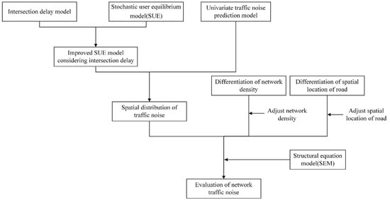
Figure 1.
The flow chart of the study.
2.2. Improved SUE Model Considering Intersection Delay
The US Highway Administration BPR function [43] in the traditional SUE model shown in Equation (1) is adopted.
In the process of traffic flow allocation, only the travel time of vehicles is considered on the road segment in the SUE model. However, the route selection behavior of travelers will be affected by traffic signal control and traffic yield rules, which encounter turning delays or idle delays at intersections. Therefore, to make the traffic allocation results more precise, the delay generated at the intersection is added to the impedance function to construct an improved SUE model.
The intersection delay is composed of the acceleration delay caused by the upstream intersection and the deceleration delay or idle delay caused by the downstream intersection, as shown in Equation (2).
where is the intersection delay of section t, (s); is the upstream intersection delay of section t, (s); is the downstream intersection delay of section t, (s).
Therefore, the expression of the road impedance function considering intersection delay is shown in Equation (3).
In this paper, the intersection delay refers to the control delay corresponding to the service level classification of signal intersections in the Code for the design of urban road engineering CJJ37-2012 [44]. The delay of the arterial road, collector road, and branch intersection are 20 s, 40 s, and 30 s, respectively.
The SUE model proposed by Fisk [45] is improved to establish the SUE model considering the delay, shown in Equation (4).
where is the road impedance function considering intersection delay; is the flow of the kth path of ; is the connection coefficient: when the kth path contains the link , take the value 1, otherwise take the value 0; is the traffic flow on road section ; is the correction factor; is the set of the OD in the network, indicates the starting point and indicates the destination.
2.3. Traffic Noise Simulation
For any receiving point P in the network, its noise will be affected by the line sources of multiple roads within the receiving radius R, as shown in Figure 2. According to the principle of energy superposition, the equivalent sound level of the receiving point is equal to the sum of the noise contribution of all road segments, shown in Equation (6).
where is the equivalent sound level of the i-th road line source, whose value is calculated by the flow-based univariate traffic noise prediction model, as shown in Equation (7); the accuracy and applicability of the model have been proved [38,39].
where is the relationship between traffic flow and speed established by the Van Aerde macro traffic flow model, and the purpose is to replace the speed variable with the flow to reduce the input parameters in the prediction model.
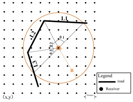
Figure 2.
Receiving point noise calculation.
Where
is the average radiated noise level at the reference point of traffic flow; is the distance from the reference point to the lane; is the distance from the calculation point to the lane; is the angle between the road segment and the line segment consisting of the noise receiver and the road segment’s endpoints (see Figure 2). is free flow speed, is the fixed space headway constant, is the first variable space headway constant, is the second variable space headway constant, is the constant for handling the relationship between and , is the maximum road traffic capacity, is the speed when the flow is the maximum road traffic capacity.
The network is divided into a grid to set noise-receiving points at the nodes. The noise at each node is calculated and displayed as a spatial distribution using the interpolation approach.
2.4. Network Structure Differentiation and Noise Evaluation Indexes
Previous studies on the influence of network characteristics on traffic noise, which mostly used data comparison methods to analyze the noise distribution differences from a qualitative perspective [28,29]. Moreover, there is no quantitative description of network characteristics [30,31]. It is difficult to quantify the effect of network characteristics on traffic noise, nor to clarify the influence mechanism. Therefore, in this paper, the influence of network density and road spatial location on traffic noise is studied by setting indicators to quantitative descriptions of the differentiation of network characteristics.
2.4.1. Network Density Considering Capacity
The network density only reflects the length of the road, which, in turn, ignores the road space width and road capacity information [46]. Therefore, the concept of Lane Area Ratio (LAR) is set to constrain the road capacity, which refers to the ratio of the actual road area to the area of the network, as shown in Equation (13). With the same LAR, the trend of traffic noise under different network density conditions is studied.
where is the sum of the actual lane areas; is the sum of the area of the region.
2.4.2. Coefficient of Spatial Inhomogeneity
The number of roads in the sub-region reflects the differentiation of the road spatial location. The network is divided into n square sub-regions, and the number of roads in each sub-region is calculated respectively. The inhomogeneity of road spatial distribution is expressed by the standard deviation of the number of roads in each sub-region, shown in Equation (14).
where N is the number of sub-regions, is the average number of roads in each sub-region, the number of roads in the i-th sub-region.
The spatial inhomogeneity coefficient of the sub-region is expressed as the ratio of the road number in the sub-region to the average of the road number, shown in Equation (15). The closer is to 1, the more uniform the distribution of roads in the sub-region.
2.4.3. Noise Evaluation Index
The evaluation index for traffic noise is proposed. Regional noise excessive rate () denotes the ratio of the area where the noise value exceeds the standard value, as shown in Equation (16).
where is the area of the i-th sound functional area; is the area lower than the noise standard value of i-th sound functional area; is the number of the sound functional area.
2.5. Structural Equation Model (SEM)
The influence of network characteristics on traffic noise is well recognized and regression models are commonly used to investigate the relationship between network characteristics and traffic noise. However, a simple regression model can only consider the direct impacts of network characteristics on traffic noise, while a structural equation model can be expressed as a path model, allowing the estimation of direct and indirect impacts of network characteristics on traffic noise through various mediating variables [47,48]. Therefore, SEM is a more powerful alternative to multiple regression analysis. In this way, it explores the influence mechanisms of network characteristics on traffic noise.
In this study, IBM SPSS is used to construct a structural equation model, which allows simultaneous testing of the total effect (TE), direct effect (DE), total indirect effect (TIE), and specific indirect effect (SIE). The TIE is the aggregate mediated effect of each SIE involved. Each SIE is associated with network characteristic indicators, traffic status indicators, and traffic noise indicators. Preacher and Hayes [49] suggested that DE, TIE, and SIE are calculated for a bootstrap sample of 5000. The impact is significant if the 95% bias-corrected confidence interval for the indirect effect parameter did not contain 0.
3. Case Study
To study the influence of network structure differentiation on traffic noise, this paper takes the network density and road spatial location differentiation as the research object. The traffic noise is simulated under the same traffic demand for different network structures. The analyses of the noise datasets for different network structures are performed using a structural equation model to clarify: (1) the extent to which the network structure differentiation influences traffic noise; (2) the mechanism and pathway to which the network structure differentiation influences traffic noise.
3.1. Case Network
3.1.1. Network Structure
To study the effect of network structure differentiation on traffic noise, a regional network in Jiading District, Shanghai, China, which belongs to the Class II sound environment functional area, was selected as the case network, as shown in Figure 3a. For further study, the network is simplified into line segments with structural parameters, and the intersections are simplified into road nodes. There are 82 nodes and 143 roads in the simplified network. Through the map software, the road structure and road length in the network are determined, as shown in Figure 3b; the label format of the information of each road is road number, road structure number, and road length. In addition, according to the code for the design of urban road engineering CJJ37-2012 [44], the grade of each road, design speed, number of lanes, road capacity, and other attributes are calibrated, as shown in Table 1.
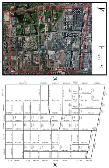
Figure 3.
Description of case network. (a) Aerial view of the network. (b) Simplified network structure.

Table 1.
Structure and number of roads.
3.1.2. Case Network Noise Data
The traffic flow on each road was obtained based on the improved SUE model. After that, the noise-receiving points are positioned in 5 m steps. The noise value at each noise-receiving point was calculated according to Equation (7) and Figure 2, and a total of 257,180 receiving point noise data were obtained. Traffic noise was displayed as a spatial distribution using the interpolation approach, as shown in Figure 4a.
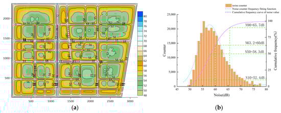
Figure 4.
Case network noise data. (a) Noise spatial distribution. (b) Noise frequency.
The frequency of noise distribution is shown in Figure 4b. The network noise conforms to the normal distribution. According to the Sound Environment Quality Standard (GB 3096-2008) [50], the environmental noise limit value of a Class II sound functional area is 60 dB in the daytime. The frequency of less than the noise limit value of 60 dB is about 63.2%, which means that there are still some areas where the noise value does not meet the standard. As can be seen from Figure 4a, these areas are concentrated on both sides of the road, especially beside the arterial road, whose traffic flow is high and speed is fast. Therefore, there is still space for optimization of the network under the consideration of traffic noise factors.
3.2. Impact of Network Density on Traffic Noise
3.2.1. Network Settings and Noise Data
In this paper, the width of the single lane is taken to be 3.5 m. The network density (ND) and Lane Area Ratio (LAR) are 6.5 km/km2 and 8.4%, respectively, in the case network. With the same LAR, the total traffic capacity of different networks remains approximately stable to meet normal traffic demands. In addition, the road distance for different network densities is determined based on the Standard for Urban Residential Area Planning and Design GB50180-2018. To keep the LAR constant, four groups of comparative networks are set by adding or removing roads in the network, and the densities of the four networks are 4.5 km/km2, 5.5 km/km2, 7.5 km/km2, and 8.5 km/km2, respectively. The network structures are shown in Figure 5.
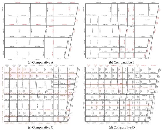
Figure 5.
Comparative network structures. (a) ND is 4.5 km/km2; (b) ND is 5.5 km/km2; (c) ND is 7.5 km/km2; (d) ND is 8.5 km/km2. ND indicates network density.
After adjusting the network structure, the improved SUE model is used to rearrange the traffic flow of the network, while controlling the total traffic volume of the network remains constant. The traffic flow of each road under different networks is obtained. Based on the road traffic flow and Equation (7), different network noise data are simulated. The traffic noise distributions of different networks are shown in Figure 6. It can be clearly shown that as the network density increases, the light green area in the noise spatial distribution map gradually increases, which means that the network noise spatial distribution is a decreasing trend. The closer to the road, the greater the noise value, especially on the arterial roads, which matches the law of the spatial distribution of noise.
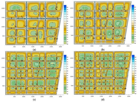
Figure 6.
Network noise distribution of four comparative networks. (a) Comparative A noise distribution. (b) Comparative B noise distribution. (c) Comparative C noise distribution. (d) Comparative D noise distribution.
According to the Sound Environment Quality Standard (GB 3096-2008) [50] and the actual situation of the network, the network region is a mixed commercial, residential, and industrial area, in which the noise daytime limit is 60 dB. The average value of traffic noise and Noise Exceedance Rate (NER) under different network densities are calculated, as shown in Figure 7.
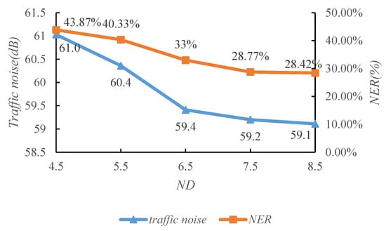
Figure 7.
Trends in traffic noise and NER.
It is clear that as the network density increases, the regional traffic noise and the NER show a significant decreasing trend. The impact of changes in network density on traffic noise is greater when the network density is low. In turn, the impact decreases as the network density increases. When the network density increases from 4.5 km/km2 to 6.5 km/km2, the decreases in traffic noise and NER are 1.6 dB and 10.87%, respectively. However, when the network density increases from 6.5 km/km2 to 8.5 km/km2, the decreases in traffic noise and NER are 0.3 dB and 4.58%, respectively.
3.2.2. Structural Equation Model (SEM) Analysis
Noise data collection points are selected at a distance of 7.5 m from the midpoint of each road. Noise and corresponding traffic parameters were obtained for 699 roads in five different density networks, such as road length, capacity (), traffic flow, and speed on the road segment. There are 699 datasets; the mean, standard deviation, and correlation matrix of each variable are shown in Table 2.
Table 2.
Means, standard deviations, and correlation matrices for all variables (N = 699).
The structural equation model is established with network density as the independent variable, traffic noise data as the dependent variable, and road characteristics and traffic parameters as the intermediate variables, as shown in Figure 8.
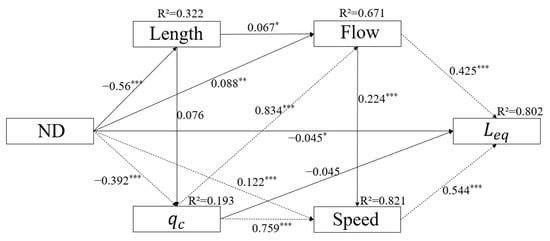
Figure 8.
Structural equation model with ND as the independent. Numbers in the figure represent standardized regression coefficients derived from the bootstrapping procedure. Dotted lines represent the important indirect pathways (p * < 0.05, p ** < 0.01, p *** < 0.001).
The fitting indexes of the model are shown in Table 3. According to the fitting indexes recommended by Hair, Mulaik, and Jackson et al. [51,52,53], all fitting indexes meet the recommended values. Therefore, the theoretical model has a good fit with the simulated data, which can be analyzed in the next step.
Table 3.
Goodness-of-fit of structural equation modelling (SEM). N = 699.
There are 14 pathways for the influence of network density on traffic noise. The parameter estimates and confidence intervals of TE, DE, TIE, and SIE are shown in Table 4, and three important indirect impact pathways are listed.
Table 4.
DE, TIE, TE, SIE of ND on .
The TE, DE, and TIE of ND on traffic noise are negative and significant; when ND increases by 1 km/km2, traffic noise decreases by 1.6 dB, 0.2 dB, and 1.4 dB, respectively. It should be noted that the DE represents the influence that ND has on noise concerning the assumption that there are no changes in the , Speed, Flow, and Length. Comparing the TIE with the DE, it is found that the TIE is far greater than the DE (86–14%), which indicates that the direct effect of changes in the physical space of the network on traffic noise is weak. On the contrary, the indirect effect on noise through changes in flow and speed is dominant.
Among the SIEs, eight pathways are significant, and the number of positive and negative significant pathways are three and five, respectively. This indicates that the IE of network density on traffic noise is uncertain. The TIE is the aggregate effect of each SIE involved. Therefore, the SIEs should be examined even when the TIE is not significant, because the mutual suppression effect between SIEs may weaken the TIE [49].
The greatest SIE S1 (ND→→Speed→): when ND increases by 1 km/km2, the decreases by 1009 (pcu/h), which then causes a reduction in speed of 3 km/h. Ultimately, also decreases by 0.8 dB (BC 95% CI [−1.067, −0.650]). The second greatest SIE S2 (ND→→Flow→): when ND increases by 1 km/km2, the decreases by 1009 (pcu/h), resulting in the reduction of flow by 507 (pcu/h), and finally the decrease in by 0.7 dB (BC 95% CI [−0.897, −0.556]).
For S1 and S2, because the network traffic demand and LAR remain constant, the decreases as the ND increases. The result is a decrease in road flow and speed. According to the noise prediction model, the noise at a certain point is positively correlated with road flow and speed. Therefore, the reduction in road flow and speed will inevitably lead to a decrease in traffic noise.
For the third greatest SIE S3 (ND→Speed→), the result is diametrically opposite to that of S1 and S2, which is positive and significant. When ND increases by 1 km/km2, the speed increases by 1 km/h, and the final increases traffic noise by 0.3 dB (BC 95% CI [0.244, 0.459]). This may be because as the network density increases, more alternative paths for vehicles are allowed, which means the traffic flow on the network is more easily dispersed and vehicles have the potential to obtain greater speeds, thus causing an increase in . In addition, all other SIEs have a weaker effect on traffic noise, with the absolute values of the estimates being less than 0.3.
In summary, network density differentiation affects traffic noise by changing the spatial distribution of traffic flow and speed, which are the key elements affecting traffic noise. The increase in the number of roads in the network gives travelers more routes to choose from, thus the additional roads relieve the traffic pressure on the network. The decrease in road traffic flow and speed caused by the increase in network density reduces traffic noise. Traffic flow can be dispersed by increasing network density to control traffic noise.
3.3. Impact of Road Spatial Location on Traffic Noise
3.3.1. Network Settings and Noise Data
The spatial location of the roads is adjusted to represent the spatial differentiation of the network. Four block-type road networks are set up to investigate the effect of spatial differentiation on traffic noise. Each network has unique road distribution forms. Network A is uniformly distributed, while B, C, and D are sparsely distributed in the center and around, respectively, as shown in Figure 9.
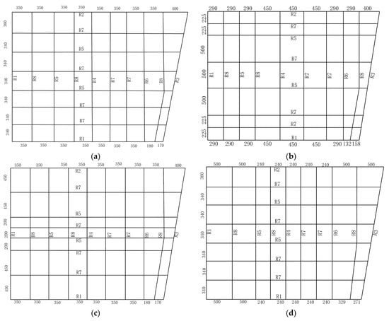
Figure 9.
Network structure settings for the impact of road spatial location. (a) Network A. (b) Network B. (c) Network C. (d) Network D.
An improved SUE model and univariate traffic noise prediction model were used to obtain noise data. The traffic noise distributions of different network structures are shown in Figure 10:
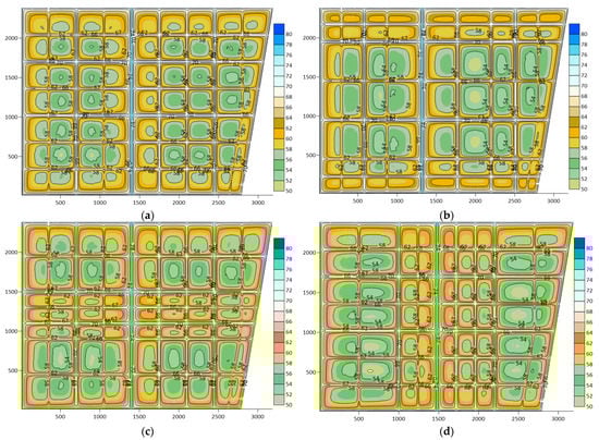
Figure 10.
Network noise distributions of different road spatial location. (a) Network A. (b) Network B. (c) Network C. (d) Network D.
In this study, the network is divided into 12 sub-regions according to 800 m steps, and the sub-regions are numbered as shown in Figure 11.
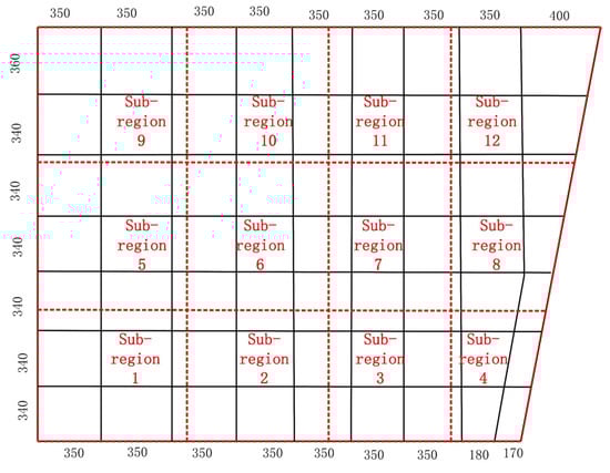
Figure 11.
Sub-regional divisions.
The four networks are divided into a total of 48 sub-regions; the COI, traffic noise, and NER of each sub-region are calculated separately, as shown in Figure 12.
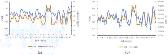
Figure 12.
COI in relation to traffic noise and NER. (a) traffic noise. (b) NER.
It is clear from the figures that the COI is significantly correlated to traffic noise and NER. The flow through the region increases because the road distribution becomes denser as the COI increases. Moreover, the region will be affected by more road noise sources, which will increase traffic noise and NER.
3.3.2. Structural Equation Model (SEM) Analysis
The network structure parameters (number of roads, COI) of each sub-region are calculated separately. Noise-receiving points are selected at 50-m spacing, and noise and traffic flow data on the roads with the greatest impact on the receiving point are acquired. A total of 9729 datasets are collected from the four networks. The mean, standard deviation, and correlation matrix of each variable are obtained, as shown in Table 5.
Table 5.
Means, standard deviations, and correlation matrices for all variables (N = 9729).
The structural equation model is established with COI as the independent variable, traffic noise data as the dependent variable, and road characteristics and traffic flow parameters as the intermediate variables, as shown in Figure 13.
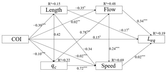
Figure 13.
Structural equation model with COI as the independent variable. Numbers in the figure represent standardized regression coefficients derived from the bootstrapping procedure. (p * < 0.05, p ** < 0.01, p *** < 0.001).
The fitting indexes of the model are listed in Table 6, and all fitting indexes meet the recommended values. Therefore, the theoretical model has a good fit with the simulated data, which can be analyzed in the next step.
Table 6.
Goodness-of-fit of structural equation modelling (SEM). N = 9729.
There are 14 pathways for the influence of COI on traffic noise. The parameter estimates and confidence intervals of TE, DE, TIE, and SIE are shown in Table 7, and three important indirect impact pathways are listed.
Table 7.
DE, TIE, TE, SIE of COI on .
The TE of COI on traffic noise is positive and significant. When the COI increases by 1, the traffic noise increases by 3.0 dB. The DE and TIE cause the traffic noise to increase by 2.3 dB and 0.7 dB, which account for 77% and 23% of the TE, respectively.
Four networks are set up to investigate the effect of road spatial location differentiation on traffic noise in the case of changing only the spatial location of roads in the network. Therefore, the traffic noise is mainly affected by the spatial location of the roads—that is, the direct effect of the COI on traffic noise dominates. This conclusion can also be verified from the results in Table 7, where the direct effect of COI on traffic noise accounts for 77% of the total effect. The traffic noise is the sum of the noise contribution of all road noise sources according to Equation (5). Thus, the receiving point is affected by more noise sources due to the denser distribution of roads, which increases traffic noise with the highest COI.
Among the SIEs, six pathways are significant, and the number of positive and negative significant pathways are four and two, respectively. The greatest SIE S1 (COI→Length→) significantly and positively effects traffic noise. When COI increases by 1, the road length decreases by 121 m, and also increases by 1.0 dB (BC 95% CI [0.900, 1.176]). The second greatest SIE S2 (COI→Length→Flow→) significantly and positively effects traffic noise. When COI increases by 1, the road length decreases by 121 m, resulting in an increase in road traffic flow of 1207 (pcu/h), which ultimately leads to an increase in of 0.7 dB (BC 95% CI [0.659, 0.808]). For the third greatest SIE S3 (COI→Length→→Flow→), the result is diametrically opposite to that of S1 and S2, which is negative. When the COI increases by 1, the road length decreases by 121 m, resulting in a decrease in road by 862 (pcu/h) and a decrease in road traffic flow by 1139 (pcu/h), which ultimately leads to a reduction in by 0.7 dB (BC 95% CI [−0.762, −0.620]).
For S1 and S2, the effects on regional traffic noise are significantly positive. When the COI increases, the number of roads in the region increases and the length of roads decreases. The essence is the same as the DE because the number of roads in the region increases, hence the traffic flow and noise sources also increase, which will increase traffic noise. However, the SIE of S1 and S2 are 1.0 dB and 0.7 dB, respectively, both of which exceed the TIE of 0.7 dB because some negative SIEs can have a suppressive effect on TIE; S3 is a typical representative of this.
For S3, when the COI increases, the road length decreases, causing a reduction in road . In addition, traffic dispersion leads to a reduction in road traffic flow as the number of roads increases, thus reducing traffic noise.
In summary, the number of regional roads determines the impact of road spatial location differentiation on traffic noise. The number of regional roads directly affects the number of noise sources and traffic flow, which determines traffic noise. Therefore, it is necessary to reasonably design the network structure in the planning stage to avoid noise pollution caused by the overconcentration of roads.
4. Discussion
The influence factors of traffic noise are attributed to road traffic flow and speed, and the urban network as a carrier determines the distribution of traffic flow and speed. Therefore, the characteristics of the urban network indirectly determine the distribution of traffic noise. The current urban planning is mainly to meet the traffic demand, and the impact on traffic noise is less considered, with minimal interaction between urban planning and noise control. This causes urban traffic noise to become a pattern of “pollution first, control later”, which not only involves huge economic costs, but also fails to fundamentally solve the traffic noise issue.
To improve network accessibility and reduce traffic congestion, the Chinese government proposed the concept of a “Small Block, Dense Network” to optimize the structure and layout of urban roads, and required that the density of urban networks be increased to 8 km/km2 by 2020. There are few studies on the effect of urban network layout changes on traffic noise. Therefore, this article focuses on the traffic noise results and influence mechanism under different network characteristics after the layout change. This study can help urban planners to understand the relationship between network characteristics and traffic noise. For example, according to our case results, when the density of the urban network is increased by 1 km/km2, the traffic noise on each road is reduced by approximately 1.5 dB. It provides a theoretical basis for traffic noise control in the planning stage.
Section 3.2 and Section 3.3 study the effect of network density and road spatial location as independent variables on traffic noise. In fact, the road spatial layout may also be diversified for different network densities due to the influence of multiple factors such as topography and population. It is also worthwhile to consider both the network density and the spatial layout of the roads. Based on our study, we can guess that the noise value is greatest when the network density is smaller and the road distribution is denser.
In addition, the urban landscape and the layout of buildings can also have an impact on traffic noise. In this study, the influences of urban landscape and building layout were not considered in order to ensure the network characteristics as the only variable, which is the direction we need to improve in our subsequent research.
5. Conclusions
Evaluate the impact of network structure differentiation on traffic noise from the perspective of network planning on the basis of typical networks in China. Traffic noise with different network structures is simulated based on an improved SUE model and a univariate traffic noise prediction model. Traffic flow is used as a mediator to study the influence mechanism of network structure on traffic noise. The study indicates that:
(1) The impact pathway of network density on traffic noise is through the changes of road traffic flow and speed caused by changes in the physical space of the network. Traffic noise decreases as the network density increases. In this case, when network density increases by 1 km/km2, traffic noise decreases by 1.6 dB. Greater network density indicates more alternative routes for travelers and dispersion of road traffic flows, which leads to the reduction of traffic noise.
(2) The impact pathway of road spatial locations on traffic noise is through the changes in the number of noise sources. Traffic noise increases alongside the dense distribution of roads. In this case, when the coefficient of inhomogeneity (COI) increases by 1, the traffic noise increases by 3.0 dB. A higher COI indicates a denser distribution of roads, which indicates that the region will be exposed to more noise sources and greater traffic flow, which leads to an increase in traffic noise.
The results show that an appropriate increase in network density and a reasonable layout of network structure can effectively alleviate traffic noise pollution. This study can provide the scientific basis for network planners to effectively control traffic noise during network design.
Author Contributions
Conceptualization, H.W.; methodology, H.W. and Z.W.; software, Z.W. and X.Y.; validation, Z.W., X.Y.; investigation, Z.W.; data curation, H.W. and J.C.; writing—original draft preparation, Z.W.; writing—review and editing, H.W., X.Y. and J.C.; visualization, X.Y.; supervision, J.C.; funding acquisition, H.W. All authors have read and agreed to the published version of the manuscript.
Funding
This work was supported by the Guangdong Basic and Applied Basic Research Foundation (2023A1515012482) and the Guangzhou Basic and Applied Basic Research Foundation (202102020670).
Institutional Review Board Statement
Not applicable.
Informed Consent Statement
Not applicable.
Data Availability Statement
The datasets used and/or analyzed during the current study are available from the corresponding author upon reasonable request.
Conflicts of Interest
The authors declare no conflict of interest.
References
- European Environment Agency. Exposure of Europe’s Population to Environmental Noise. Available online: https://www.eea.europa.eu/ims/exposure-of-europe2019s-population-to (accessed on 14 February 2023).
- Alina, P.; Jose, L. Dynamic evaluation of traffic noise through standard and multifractal models. Symmetry 2020, 12, 1857. [Google Scholar]
- European Environmental Agency. Country Fact Sheets: Romania. In Noise in Europe 2017 Overview of Policy-Related Data; European Environmental Agency: Bruxelles, Belgium, 2017. [Google Scholar]
- Ministry of Ecology and Environment of the People’s Republic of China. China Environmental Noise Prevention and Control Annual Report 2020; Ministry of Ecology and Environment of the People’s Republic of China: Beijing, China, 2020.
- World Health Organization. Environment Noise Guidelines for the European Region. Available online: https://www.who.int/europe/publications/i/item/9789289053563 (accessed on 14 February 2023).
- Guski, R.; Schreckenberg, D.; Schuemer, R. WHO environmental noise guidelines for the european region: A systematic review on environmental noise and annoyance. Int. J. Environ. Res. Public Health 2017, 14, 1539. [Google Scholar] [CrossRef] [PubMed]
- Kempen, E.; Casas, M.; Pershagen, G.; Foraster, M. WHO environmental noise guidelines for the european region: A systematic review on environmental noise and cardiovascular and metabolic effects: A summary. Int. J. Environ. Res. Public Health 2018, 15, 397. [Google Scholar] [CrossRef] [PubMed]
- Basaner, M.; Mcguire, S. WHO environmental noise guidelines for the european region: A systematic review on environmental noise and effects on sleep. Int. J. Environ. Res. Public Health 2018, 15, 591. [Google Scholar] [CrossRef]
- Tom, C.; Rina, S.; Heresh, A.; Claus, B.; Zorana, J.A. Long-term exposure to road traffic noise and all-cause and cause-specific mortality: A Danish Nurse Cohort study. Sci. Total Environ. 2022, 820, 153057. [Google Scholar]
- Karbalaei, S.; Karimi, E.; Naji, H.; Ghasempoori, S.; Hosseini, S.; Abdollahi, M. Investigation of the traffic noise attenuation provided by roadside green belts. Fluct. Noise. Lett. 2015, 14, 1550036. [Google Scholar] [CrossRef]
- Ow, L.; Ghosh, S. Urban cities and road traffic noise: Reduction through vegetation. Appl. Acoust. 2017, 120, 15–20. [Google Scholar] [CrossRef]
- Ilgurel, N.; Akdag, N.; Akdag, A. Evaluation of noise exposure before and after noise barriers, a simulation study in Istanbul. Environ. Eng. Manag. J. 2016, 24, 293–302. [Google Scholar] [CrossRef]
- Rochat, J.; Fleming, G. Validation of FHWA’s Traffic Noise Model (TNM): Phase 1; Department of Transportation: Washington, DC, USA, 2002.
- Givargisa, S.; Mahmoodi, M. Converting the UK calculation of road traffic noise (CORTN) to a model capable of calculating LAeq,-1h for the Tehran’s roads. Appl. Acoust. 2008, 69, 1108–1113. [Google Scholar] [CrossRef]
- Sakamoto, S. Road traffic noise prediction model ‘ASJ RTN-Model 2018’: Report of the research committee on road traffic noise. Acoust. Sci. Technol. 2020, 41, 529–589. [Google Scholar] [CrossRef]
- Cai, M.; Zhong, S.; Wang, H.; Chen, Y.; Zeng, W. Study of the traffic noise source intensity emission model and the frequency characteristics for a wet asphalt road. Appl. Acoust. 2017, 123, 55–63. [Google Scholar] [CrossRef]
- Li, F.; Lin, Y.; Cai, M.; Du, C. Dynamic simulation and characteristics analysis of traffic noise at roundabout and signalized intersections. Appl. Acoust. 2017, 121, 14–24. [Google Scholar] [CrossRef]
- Abdur-Rouf, K.; Shaaban, K. Development of prediction models of transportation noise for roundabouts and signalized intersections. Transp. Res. Transp. Environ. 2022, 103, 103174. [Google Scholar] [CrossRef]
- Mot, M.; Gar, W. Statistical model for traffic noise prediction in signalised roundabouts. Bull. Pol. Acad. Sci. Technol. Sci. 2020, 68, 937–948. [Google Scholar]
- Khajehvand, M.; Rassafi, A.A.; Mirbaha, B. Modeling traffic noise level near at-grade junctions: Roundabouts, T and cross intersections. Transp. Res. Transp. Environ. 2021, 93, 102752. [Google Scholar] [CrossRef]
- Jonathan, R.; Peter, W.; Theresa, Z. The Effect of Speed Limits and Traffic Signal Control on Emissions. In Proceedings of the 11th International Workshop on Agent-based Mobility, Traffic and Transportation Models, Methodologies and Applications, Porto, Portugal, 22–25 March 2022. [Google Scholar]
- Lu, X.; Kang, J.; Zhu, P.; Cai, J.; Guo, F.; Zhang, Y. Influence of urban road characteristics on traffic noise. Transp. Res. Transp. Environ. 2019, 75, 136–155. [Google Scholar] [CrossRef]
- Wang, S.; Lo, E.; Liang, C.; Chao, K.; Bao, B.; Chang, T. Temporal and spatial variations in road traffic noise for different frequency components in metropolitan Taichung, Taiwan. Environ. Pollut. 2016, 219, 174–181. [Google Scholar] [CrossRef]
- Ritesh, V.; Chandan, K.; Manoj, K. Assessment of Traffic Noise on Highway Passing from Urban Agglomeration. Fluct. Noise Lett. 2014, 13, 1450031. [Google Scholar]
- Liu, T. The Urban Road Traffic Noise Impact Factor and Spreading Regularity Analysis. Master’s Thesis, Chang’an Unversity, Xi’an, China, 2009. [Google Scholar]
- Wang, B.; Kang, J. Effects of urban morphology on the traffic noise distribution through noise mapping: A comparative study between UK and China. Appl. Acoust. 2011, 72, 556–568. [Google Scholar] [CrossRef]
- Salomons, E.M.; Berghauser, P.M. Urban traffic noise and the relation to urban density, form, and traffic elasticity. Landsc. Urban Plan. 2012, 108, 2–16. [Google Scholar] [CrossRef]
- Sheng, N.; Tang, U.W. Spatial analysis of urban form and pedestrian exposure to traffic noise. Int. J. Environ. Res. Public Health 2011, 8, 1977–1990. [Google Scholar] [CrossRef] [PubMed]
- Tang, U.W.; Wang, Z.S. Influences of urban forms on traffic-induced noise and air pollution: Results from a modelling system. Environ. Model. Softw. 2007, 22, 1750–1764. [Google Scholar] [CrossRef]
- Li, M.; Lu, X.; Liu, J. Comparative study on spatial changes of traffic noise under different planning concepts. Audio Eng. 2021, 45, 5–9. [Google Scholar]
- Lu, X.; Cai, J.; Zhu, P. Comparison of the Influences of Urban Road Networks on Traffic Noises—A Case Study of the Typical Area in Dalian. Noise Vib. Control. 2019, 39, 147–151. [Google Scholar]
- Shahla, T.; Atefeh, C.; Mozhgan, A.; Minoo, M. Acoustics in urban parks: Does the structure of narrow urban parks matter in designing a calmer urban landscape? Front. Earth Sci. 2020, 14, 512–521. [Google Scholar]
- Efstathios, M.; Jian, K. Relationship between green space-related morphology and noise pollution. Ecol. Indic. 2017, 72, 921–933. [Google Scholar]
- Ligia, T.; Marta, O.; Jose, F. Urban form indicators as proxy on the noise exposure of buildings. Appl. Acoust. 2014, 76, 366–376. [Google Scholar]
- Wang, H.; Gao, H.; Cai, M. Simulation of traffic noise both indoors and outdoors based on an integrated geometric acoustics method. Build Environ. 2019, 160, 106201. [Google Scholar] [CrossRef]
- Cai, M.; Zou, J.F.; Xie, J.M.; Ma, X.L. Road traffic noise mapping in Guangzhou using GIS and GPS. Appl. Acoust. 2015, 87, 94–102. [Google Scholar] [CrossRef]
- Lan, Z.Q.; Cai, M. Dynamic traffic noise maps based on noise monitoring and traffic speed data. Transp. Res. Transp. Environ. 2021, 94, 102796. [Google Scholar] [CrossRef]
- Chen, L.; Sun, B.; Wang, H.B.; Li, Q.R.; Hu, L.; Chen, Z. Forecast and control of traffic noise based on improved UE model during road network design. Appl. Acoust. 2020, 170, 107529. [Google Scholar] [CrossRef]
- Wang, H.B.; Sun, B.; Chen, L. An optimization model for planning road networks that considers traffic noise impact. Appl. Acoust. 2022, 192, 108693. [Google Scholar] [CrossRef]
- Wang, H.B.; Chen, H.J.; Cai, M. Evaluation of an urban traffic noise-exposed population based on points of interest and noise maps: The case of Guangzhou. Environ. Pollut. 2018, 239, 741–750. [Google Scholar] [CrossRef] [PubMed]
- Wang, H.B.; Wu, Z.Y.; Chen, J.C.; Chen, L. Evaluation of road traffic noise exposure considering differential crowd characteristics. Transp. Res. Transp. Environ. 2022, 105, 103250. [Google Scholar] [CrossRef]
- Cai, M.; Lan, Z.Q.; Zhang, Z.W.; Wang, H.B. Evaluation of road traffic noise exposure based on high-resolution population distribution and grid-level noise data. Build. Environ. 2019, 147, 211–220. [Google Scholar] [CrossRef]
- Federal Highway Administration. FHWA Highway Traffic Noise Prediction Model; Federal Highway Administration: Washington, DC, USA, 1978.
- Ministry of Housing and Urban-Rural Construction of the People’s Republic of China. CJJ37-2012 Code for Design of Urban Road Engineering; Ministry of Housing and Urban-Rural Construction of the People’s Republic of China: Beijing, China, 2012.
- Fisk, C. Some developments in equilibrium traffic assignment. Transp. Res. Methodol. 1980, 14, 243–255. [Google Scholar] [CrossRef]
- Cheng, P.T. The Study on Grade Proportion of Urban Road Network under the Concept of Narrow Road with Dense Network. Master’s Thesis, Huazhong University of Science and Technology, Wuhan, China, 2018. [Google Scholar]
- Fyhri, A.; Klaeboe, R. Road traffic noise, sensitivity, annoyance and self-reported health-a structural equation model exercise. Environ. Int. 2009, 35, 91–97. [Google Scholar] [CrossRef]
- Hong, J.Y.; Jeon, J.Y. Influence of urban contexts on soundscape perceptions: A structural equation modeling approach. Landsc. Urban Plan. 2015, 141, 78–87. [Google Scholar] [CrossRef]
- Preacher, K.J.; Hayes, A.F. Asymptotic and resampling strategies for assessing and comparing indirect effects in multiple mediator models. Behav. Res. Methods 2008, 40, 879–891. [Google Scholar] [CrossRef]
- GB 3096–2008; Environmental Quality Standard for Noise. China’s State Environmental Protection Administration: Beijing, China, 2008.
- Hair, J.; Black, W.; Babin, B.J. Multivariate Data Analysis, 7th ed.; Prentice Hall: Englewood Cliffs, NJ, USA, 2009. [Google Scholar]
- Mulai, S.; James, L. Evaluation of goodness-of-fit indices for structural equation models. Psychol. Bull. 1989, 105, 430–445. [Google Scholar] [CrossRef]
- Jackson, D.L.; Gillaspy, J.A.; Purc-Stephenson, R. Reporting practices in confirmatory factor analysis: An overview and some recommendations. Psychol. Methods 2009, 14, 6–23. [Google Scholar] [CrossRef] [PubMed]
Disclaimer/Publisher’s Note: The statements, opinions and data contained in all publications are solely those of the individual author(s) and contributor(s) and not of MDPI and/or the editor(s). MDPI and/or the editor(s) disclaim responsibility for any injury to people or property resulting from any ideas, methods, instructions or products referred to in the content. |
© 2023 by the authors. Licensee MDPI, Basel, Switzerland. This article is an open access article distributed under the terms and conditions of the Creative Commons Attribution (CC BY) license (https://creativecommons.org/licenses/by/4.0/).