Optimized Deep Learning with Learning without Forgetting (LwF) for Weather Classification for Sustainable Transportation and Traffic Safety

Abstract

Unfortunately, accidents caused by bad weather have regularly made headlines throughout history. Some of the more catastrophic events to recently make news include a plane crash, ship collision, railway derailment, and several vehicle accidents. The public’s attention has been directed to the severe issue of safety and security under extreme weather conditions, and many studies have been conducted to highlight the susceptibility of transportation services to environmental factors. An automated method of determining the weather’s state has gained importance with the development of new technologies and the rise of a new industry: intelligent transportation. Humans are well-suited for determining the temperature from a single photograph. Nevertheless, this is a more challenging problem for a fully autonomous system. The objective of this research is developing a good weather classifier that uses only a single image as input. To resolve quality-of-life challenges, we propose a modified deep-learning method to classify the weather condition. The proposed model is based on the Yolov5 model, which has been hyperparameter tuned with the Learning-without-Forgetting (LwF) approach. We took 1499 images from the Roboflow data repository and divided them into training, validation, and testing sets (70%, 20%, and 10%, respectively). The proposed model has gained 99.19% accuracy. The results demonstrated that the proposed model gained a much higher accuracy level in comparison with existing approaches. In the future, this proposed model may be implemented in real-time.

1. Introduction

Weather phenomenon analysis plays a critical role in environmental monitoring, weather forecasting, and ecological quality evaluation [1], not to mention that various weather events have multiple impacts on farming. Hence, it is beneficial to agricultural planning if meteorological events are correctly differentiated [2]. In addition, weather phenomena dramatically affect car-assisted driving systems and our day-to-day lives, impacting things such as the technology we wear, use to travel, and rely on for energy [3,4,5]. Many visual designs, including outdoor video surveillance, are similarly vulnerable to the effects of weather on their functioning [6]. As a result, it is easy to deduce that establishing clear categories for weather occurrences is crucial for gaining insight into climate conditions and making more accurate weather predictions [7].

Making a weather forecast involves observation, analysis, and prediction. Weather conditions, such as barometric pressure, temperature, humidity, wind speed, and cloud cover, are all considered throughout these times [8]. The number of clouds in the sky, also known as cloud coverage, cloudage, cloud amount, or cloudiness, is a significant influence [9]. Traditional meteorology typically employs cloud coverage during the observation phase by dispatching personnel to the field to take pictures, during the analysis phase by stationing expert personnel to analyze the images taken during the observation phase, and during the prediction phase by calculating the desired outcome of a weather forecast using all of the data mentioned above, including cloudage [10]. It is generally accepted that a conventional weather service can make predictions with an accuracy of around 90% for five days, 80% for seven days, and 50% for ten days. Advanced technologies and techniques are used in the apparatus and methods of analysis and prediction [11]. However, the result is still far from near-zero mistakes, especially over extended periods. When humans are impacted by extraordinary conditions, such as the current COVID-19 pandemic, human-based systems become much more error-prone than typical. During the pandemic, meteorology mistakes increased since field workers and specialists at meteorology stations did not show up to work consistently, causing difficulties in making accurate weather forecasts.

Meteorological agencies worldwide use various methods to calculate cloud cover manually, but in Turkey, the process goes as follows. The first step is for field observers to send cloud photos to the stations from the ground, which can be observation towers or balloons. The gathered images are then divided into eight sections, each of which is reviewed separately by human specialists. Each component might end up in one of three ways: To determine whether or not it is cloudy, experts look at the percentage of cloud cover in the sky; if it is more than 50%, the weather forecasters consider the day dirty; if it is less than 50%, the weather forecasters consider the day clear [12]. The image is discarded as noisy if the picture contains no sky parts and only data unrelated to weather forecasting. Once the cloudiness of each fragment has been established, the non-noise pieces are reassembled into the original picture. The picture is deemed cloudy if cloudy components constitute fifty percent or more of the total or precise otherwise [13].

Instead of collecting picture data daily or weekly and evaluating it with human specialists, training a large dataset with steadily rising volume and processing it via a well-founded deep learning architecture will provide a fresh viewpoint and vastly improve prediction accuracy. With big data and AI technology, a task that previously required specialized human labour may be reduced to a simple computation [14].

Systems trained using deep learning may automatically assign tags to new data based on what it has learnt from previously tagged data sets. The next iteration of ML, called “deep learning”, is built from interconnected layers of computation that learn to make predictions and processes using the data they have been given. While deep learning, machine learning, and artificial intelligence (AI) each have distinct meanings, they may all be understood as subsets of each other thanks to their shared methodology and architecture [15].

Conventional techniques of meteorological phenomenon categorization often rely on human observation. However, the time-consuming and error-prone process of using artificial visual differentiation between meteorological occurrences is a problem. Therefore, it is critical to advance accurate, effective, and automated methods of categorizing meteorological events. In recent years, a collaborative learning method has been employed for the two-class weather categorization (sunny and cloudy). Not only has that but a straightforward linear classifier has been used to divide scenes into those with and without fog correctly. Recent advances in machine learning have opened up new avenues of inquiry for its potential use by scholars. Through the use of feature extraction and K-Nearest Neighbor, it has accomplished weather condition detection, a necessary step in the process of identifying meteorological occurrences. However, traditional machine learning approaches to weather phenomenon detection cannot successfully learn the specifics of weather events. The research question that arises here is, “Can the modified Yolov5 model classify the weather for the sake of avoiding road accidents in improving quality of life?” The critical contribution of this research is as follows:

• This research aims to suggest an automated workflow that can automatically accurately identify and classify weather. The proposed Model’s initial training images were compiled using the autoargumention, which can determine the textural connection among an image’s pixels. This research utilizes the online weather dataset.
• The modified Yolov5 Model distinguishes the different classifications of weather.
• The proposed technique and existing methods, i.e., Yolov5 model and SDG optimizer, hybrid Learning without forgetting, were implemented over Google Cololab and compared based on comparison parameters, i.e., Sensitivity, precision, Accuracy, and similarity index values.
• The proposed Model achieves better precision, Accuracy, and Sensitivity than existing methods.

The complete research is organized as follows: Section 2 covers the related work, Section 3.1 covers the details of the Dataset, Section 3.2 explains the proposed method, Section 3.3 explains Proposed Methodology, Section 4.1 covers the experimental settings, Section 4.2 covers Weather-specific Features and Section 4.3 describe Classification Measures, and Section 5 covers the conclusion and future works.

2. Review of Literature

Wang et al. [16] described and assessed a nonlinear Support Vector Machine-based model for predicting atmospheric visibility based on continuous data from the unique autonomous weather stations ROSA along the Beijing airport expressway in 2006 and 2007. According to the evaluation, the Support Vector Machine-based forecast model performed admirably. More than 90% of forecast categorization errors are within one level, while predictions of air visibility are only 40% accurate based on actual data (including equality). In addition, future 3–48 h projected atmospheric visibility functioned consistently. These flawless predictions prove that the Support Vector Machine approach is well-suited to handling the nonlinear connection between atmospheric transparency and climatic variables.

Hongwei et al. [17] offer a new categorization learning system that employs multi-objective GA. Machine learning is first made more generalizable and interpretable by using a supervised segmentation approach to make judgments about the continuous properties of samples. As a bonus, multi-objective GA incorporates a comparison and selection process derived from partial order in set theory. They improve one’s capacity to choose favourable chromosomes. The novel method is employed for microthermal weather forecasting in northern Zhejiang province. Based on the results of the experiments, it possesses superior intelligence and precision.

It is proposed by Hongwei et al. [18] that algorithms be developed to predict the power production of PV systems using weather categorization and support vector machines (SVM). Implementation at a 20 kW capacity PV station in China demonstrates the efficacy and promise of the suggested forecasting model for grid-connected PV systems.

Zhang et al. [19] describe a technique for multi-class weather classification in every circumstance. Their methods can extract many meteorological characteristics and require enough processing time. They use multiple kernel learning to train an adaptable classifier to combine these characteristics into high-dimensional vectors. The MWI (Multi-class Weather Image) set is a collection of 20,000 photographs taken in various weather conditions. The suggested technique has been shown to successfully recognize weather conditions on the MWI dataset.

Four examples from forthcoming films with lousier weather circumstances were included in their newly developed railway transportation dataset to increase the safety of railway transportation in real-world weather situations. Considering the nature of railway transportation photos, which consist primarily of a single item against a uniform background, the available options for identifying the weather are restricted. Wang et al. [20] also gathered a multi-class meteorological dataset to enhance the classification model’s generalization capability. For the purpose of avoiding enlisting complex pre-processing processes and collecting a discriminating characteristic for each weather scenario, they showed on publicly available meteorological datasets and their dataset that the proposed framework outperformed the current gold standard approaches.

To render their method immune to global intensity transfer, Lu et al. [21] suggest a new data augmentation scheme to significantly enhance the training data, which is then utilized for training a latent SVM framework. Extensive experimental work has been done to prove the efficacy of their approach. This article enhances accuracy by up to 7–8% compared to their earlier work, which relied solely on a CNN classifier. The classifier’s executable may be downloaded alongside the weather picture dataset.

Li et al. [22] propose utilizing generative adversarial networks (GAN) to supplement existing data. It may complement and complete a wide variety of visual data. To address this problem, they developed a system that uses deep convolution generative adversarial networks (DCGANs) to produce pictures distributed evenly over the dataset and a Convolutional Neural Network (CNN) model to check the accuracy of the generated classifications. They also provide an assessment approach on three benchmark datasets to test DCGAN’s accuracy. The empirical findings show that high-quality weather images may be created using DCGAN on weather data sets. Classification accuracy also increased when we implemented the DCGAN-based data augmentation technique.

Zhang et al. [23]’s multimodal adaptive regression spline (MARS) model accounted for complex weather conditions over the year. Its excellent computing efficiency and ability to be updated progressively make it suitable for EIM activities. The outcomes of the tests and analysis show that the innovative model is more accurate, flexible, and efficient.

According to Wang et al. [24], it is crucial to industry and human survival to quickly and accurately identify different types of weather. The dataset used in this paper consists of nine different categories of ground-level weather photographs, each of which was gathered and categorized. It has been shown experimentally that the strategy outperforms state-of-the-art methods in weather recognition.

Five types of meteorological elements were identified in the photographs by Bai et al. [25]. We propose a novel satellite image classification framework called a multimodal auxiliary network that takes advantage of these different modalities for detecting clouds and weather systems (MANET). MANET’s three components are a convolutional neural network for extracting features from images, a perceptron for extracting features from weather data, and a layer-level multimodal fusion module. Meteorological components and satellite photos are only two examples of multimodal data that MANET effectively combines. Based on the findings of the experiments, it is clear that MANET can improve the categorization of satellite photos of weather systems, clouds, and land cover.

Alem et al. [26] recommended constructing a convolutional neural network feature extractor (CNN-FE) for the LCLU classification system from scratch, transferring knowledge from other models, and then fine-tuning it using remotely sensed pictures for evaluation and comparison. This study examines and compares deep learning techniques for distant sensing picture categorization. They created and trained many deep learning models using the UCM dataset and then reached their results using several measures to assess performance.

To forewarn the time duration and specific magnitude of peak load, Deng et al. [27] offer a model based on the Bagging-XGBoost algorithm for identifying extreme weather and making short-term load forecasts. To begin, they add the concept of Bagging to the Extreme Gradient Boosting (XGBoost) method to lower output variance and increase generalization capacity. After then, the input weight of the model is tweaked by analyzing the mutual information (MI) between weather-influencing components and load to follow weather shifts better. The next step is to develop the extreme weather detection model by considering the load, weather, and timing elements to find the peak load occurrence range. Finally, a very accurate short-term load forecasting model is constructed by selecting a customized training set based on weighted similarity.

Table 1. Summary of existing work.

S. No.	Paper	Method	Dataset	Result
1	Wang et al. [16]	SVM	Weather stations ROSA	90% of forecast classification errors
2	Hongwei et al. [17]	GA	Meteorological data in Northern Zhejiang	75% correct rate
3	Shi et al. [18]	SVM	PV power system in south China	8.64 MREdata (%)
4	Zhang et al. [19]	multiple kernel learning	MWI (Multi-class Weather Image)	Accuracy 0.5944
5	Wang et al. [20]	Multitask learning	multi-class weather dataset	MSE 0.79167
6	Lu et al. [21]	CNN	weather dataset having 10,000 images	Accuracy 91.4%
7	Li et al. [22]	Generative adversarial networks (GAN)	MWI, MWD datasets	Accuracy 0.9809
8	Zhang et al. [23]	multivariate adaptive regression spline	China radiation date dataset	MAE 0.689
9	Wang et al. [24]	ResNet and DenseNet	12,000 pictures dataset	Accuracy 72.25%
10	Bai et al. [26]	Multimodal Information Fusion	LSCIDMR dataset	Accuracy 98.46%
11	Alem et al. [25]	Convolutional Neural Network	UCM dataset	Precision 0.89
12	Deng et al. [27]	XGBoost algorithm	1120 pictures dataset	MAPE 10%

depicts the summary of existing work.

3. Dataset and Experiment

3.1. Dataset

This dataset includes five weather classes gleaned from the aforementioned diverse sources; nevertheless, given the nature of the data, any weather classification system must be able to process photos with varying degrees of naturalism. Including the validation photos, the dataset has around 1500 labels [28]. Prints range in size because images do not have uniform proportions. Images captured during different types of weather are stored in their respective folders according to the labelled class [29]. The following weather conditions have been assigned numerical values, from 0 (very poor) to 4 (very good), for each of the images:

• 0—Cloudy
• 1—Foggy
• 2—Rainy
• 3—Shine
• 4—Sunrise

3.2. Methods

Neural networks, part of the more significant subject of machine learning, are the foundation of cutting-edge deep learning methods. Input, hidden, and output layers are all components of a node layer [30]. Each network node is correlated with a weight and a threshold. Even while feedforward networks were the primary subject of that article, many other types of neural nets may perform better on specific tasks or with certain inputs. Naturally, recurrent neural networks are more frequently utilized in NLP and voice recognition tasks, whereas CNNs are more commonly used in computer vision and classification applications. Picture object recognition was a time-consuming and arduous process that needed human feature extraction methods before the development of CNNs [31].

This section will compare and contrast convolutional neural networks (CNNs) and neural networks. Traditional neural networks have one major drawback compared to artificial neural networks: they cannot be easily scaled [32]. Regular NNs may be adequate for smaller pictures with fewer colour channels. However, a more extensive and expensive NN is required as the size and complexity of an image raises the requirement for processing power and resources. There’s also the issue of overfitting [33]. NN may pick up on the background noise, which will negatively impact its performance on test data [34]. However, a CNN’s nodes link to one another and are weighted at each layer. Parameter sharing describes this scenario. As a result of this procedure, CNN systems use less processing power than NN systems [35]. Multiple layers in a network can improve accuracy over a single one. Depending on the task at hand, deep learning can employ either RNNs or CNNs [36].

3.2.1. Architecture

As the object data travels through the CNN’s multiple levels, the CNN gradually learns its features. Because of this direct (and deep) learning, feature extraction may be done automatically (feature engineering) [37]. Due to their usage of shared parameters, CNNs are far more efficient computationally than traditional NNs. The models are portable, allowing them to function on anything from desktop computers to mobile phones. The CNN’s last layer is an FC layer, where it learns to identify the picture or object it has been given [38]. By using convolution, a picture is passed through several such filters. Each filter performs its function on the image and then gives the results to the next filter in the chain. As more and more layers are added and trained, the process of identifying characteristics is repeated hundreds, if not thousands, of times. Finally, the CNN can recognize the complete object thanks to all the picture data it has processed through its many layers [39]. When compared to other types of neural networks, convolutional networks excel in processing inputs that are images, voices, or sounds. Their layers come in three distinct varieties:

• Convolutional layer
• Pooling layer
• Fully-connected (FC) layer

The first layer of a convolutional network is the convolutional layer. The fully-connected layer comes last in a neural network architecture, following any number of layers that may or may not be convolutional or pooling layers [40]. Adding more layers to the CNN allows it to recognize more subtle differences in a picture. Initial layers analyze data for essential characteristics, such as colours and edges [41].

3.2.2. Convolutional Layer

The convolutional layer is the first layer. Input data is taken as a 3D pixel matrix with RBG factors, a filter/kernel as a feature detector, and a feature map. Part of the image is represented by a weighted array that takes up two dimensions (2D) in the feature detector [42]. Dot products between the input and filter are convolved to produce the final output.

To further refine the results, we may add a second convolution layer on top of the first one, as discussed before. Because the last layers may now access the information in the earlier layers’ receptive fields, CNN’s structure can take on a hierarchical form [43].

3.2.3. Pooling Layer

Dimensionality reduction is carried out through pooling layers, also known as downsampling, by decreasing the number of input parameters. Instead, the kernel aggregates the values in the receptive field to form the output array. Most forms of pooling fall into one of two categories [44].

Maximum pooling involves choosing the input pixel with the highest value and sending it to the output array when the filter scans the input. As a side note, this method is typically employed more frequently than average pooling [45]. Moving the filter over the information causes it to moderate the values inside the receptive field and transfer those averages to the output array. Despite the fact that the pooling layer causes the CNN to lose a lot of information, it does have certain advantages. They aid in streamlining processes, boosting productivity, and lowering overfitting danger [46].

3.2.4. Fully-Connected Layer

In the fully-connected layer, each node in the output layer directly connects to a node in the layer below it. This layer categorizes using the characteristics of the preceding layers’ various filters [47]. In 2015, Joseph Redmond et al. introduced YOLO to address the issues with object recognition models. The network must be run forward once for the predictions to be made.

3.2.5. Disadvantages of YOLO

• It has comparatively low recall and more localization error compared to faster R_CNN.
• It struggles to detect close objects and detect small objects [27].

Learning-without-Forgetting (LwF) is a combination of distillation networks and fine-tuning. The transfer learning technique is considered a particular case of incremental learning. LwF is a technique in which the old and new tasks are different, whereas, in incremental learning, the old and new jobs can also be the same, popularly called domain adaptation [48]. Learning without forgetting is one of the methods to solve multitasking learning. If a model is trained to solve problem X and then after sometimes we need the model to solve new problem Y without forgetting the problem X, then we use LwF. Transfer learning uses a trained model to solve another task and may ignore the initial charge. For example, we use this model initially used to teach how to classify a cat or dog to a new job that is now used to classify a goat or a cow. There are several approaches for multitasking learning, but LwF seems to be the most appropriate one.

Figure 1 illustrates the working theory of familiar multitask learning methods. Let’s assume a pre-trained model (a) with m old tasks, and we want to add a new job to this pre-trained model. Fine-tuning approach inserts a branch for the new study at the end and then retrains the backbone. Feature Extraction technique adds more layers in the new-task addition and trains only this branch.

Figure 2 illustrates the working theory of the Learning-without-Forgetting (LwF) method. To better understand the working of LwF, a flowchart is illustrated in Figure 3.

The joint Training method inserts a new branch for the novel task and retrains the entire network. In the case of only new-task data, Learning without Forgetting (LwF), as shown in Figure 3, learns a network that can perform well on both old and new tasks. LwF strategy is a kind of continual learning technique that only uses the latest data and assumes that past data (used to pre-train the network) is not available.

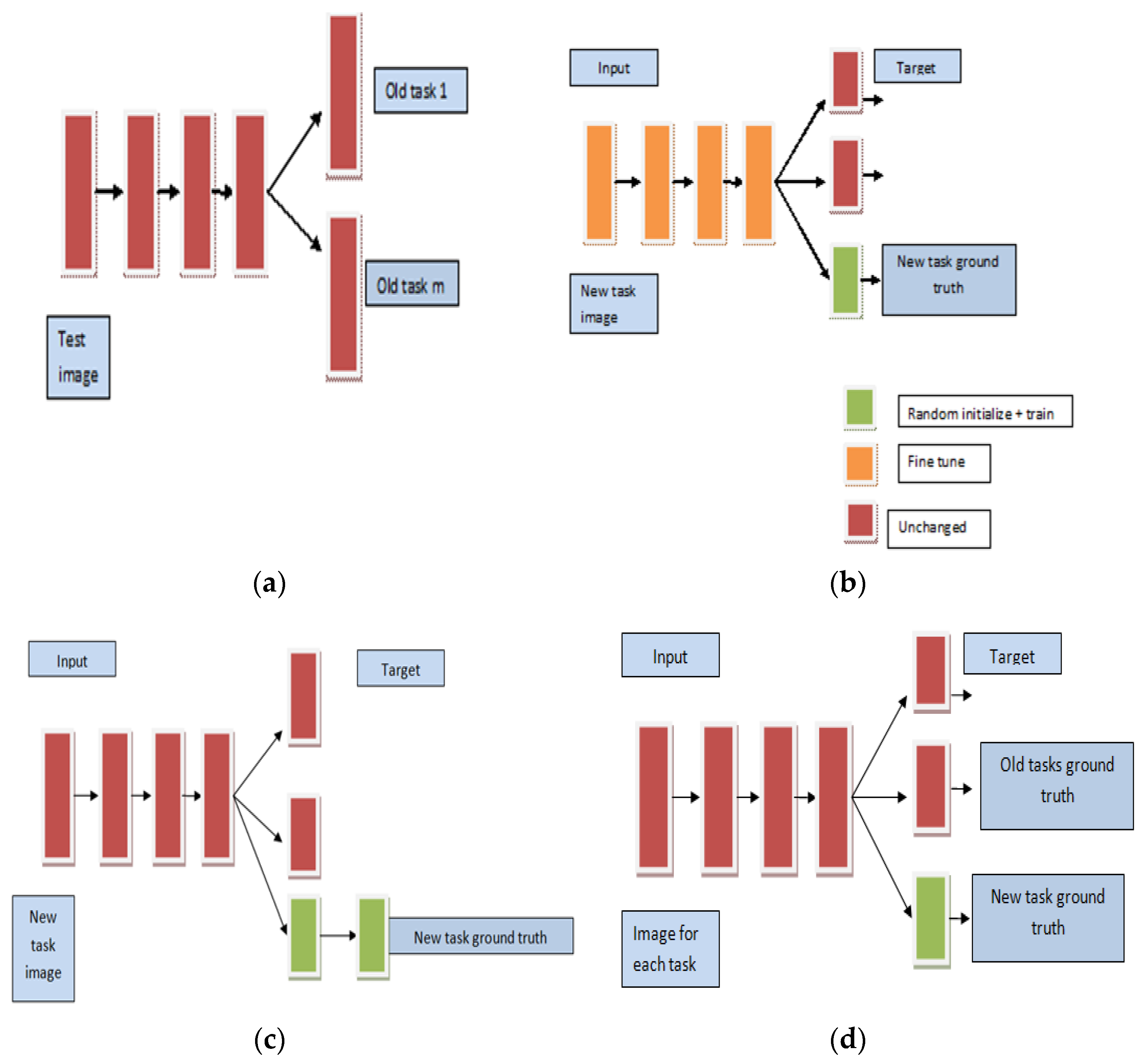
3.3. Proposed Methodology

YOLO recommends using an end-to-end neural network to anticipate both bounding boxes and class probabilities simultaneously. A schematic depicting how YOLO may be used to identify many objects simultaneously is shown in Figure 4.

Compared to other algorithms, YOLO’s predictions are performed entirely by a single, fully linked layer. When running a picture via the YOLO algorithm, it is first divided into N grids, each of which is an SxS square of the same size.

The pseudocode for YOLO is given below.

Step 1.

If many options exist, choose the one where the goal function is the highest.

Step 2.

Next, it should examine this box’s overlap (Intersection over Union, IOU) with others.

$$Intersection of union=\frac{Area of overlap}{Area of union}$$

(1)

Step 3.

Any boxes whose boundaries overlap by more than half (intersection > union) should be discarded.

Step 4.

Follow it up by moving on to the next-highest objectiveness rating.

Step 5.

Finally, do it again from step 4.

Every one of these N grids is in charge of finding and pinpointing whatever happens in it. To that end, these grids provide predictions about the label and presence probability of objects in a given cell and their bounding box coordinates relative to the cell’s own coordinates for weather images.

4. Experimental Results

4.1. Experiment Setting

The Collaboratory’s Tesla K80 GPU was equipped with a laptop with an Intel Core i3-4000M CPU (Intel Corporation, Mountain View, CA, USA) running at 2.40 GHz and 4 GB of RAM for the experiments. For this experiment, we used the Python libraries Keras 2.20.0 and TensorFlow 2.12.0, both of which are open-source DL software packages. In addition, we analysed the performance measures using the scikit-learn statistical program. Training, validation, and testing sets are being partitioned into 70%, 20%, and 10%, respectively.

4.2. Weather-Specific Features

The edges of objects in a picture are often selected as features in the traditional image classification procedure. However, this is impossible when attempting to classify images based on meteorological conditions. Therefore, we must adopt other standards. We accessed the characteristics of photographs taken in various weather circumstances and used that data to compile a set of six carefully selected attributes related to weather.

(1)

Brightness: The level of illumination is a crucial characteristic of pixels. Pictures taken on clear days tend to have a higher luminance than those taken in the presence of clouds or fog. Luma Brightness was introduced by Sergey Bezryadin et al. [19] as an efficient technique to compute brightness replacements, and its corresponding formula is given in Equation (1):

$$B^{\prime }=0.114b+0.587g+0.299r$$

(2)

where B’ is the Luma brightness value, r, g, and b are stimulus RGB coordinates.

(2)

Contrast is the difference between a picture’s brightest and darkest parts or the range of pixel intensities. The greater the disparity between the two, the greater the contrast. Using the encoded contrasts as a percentile in picture saturation, we may determine the contrast. Equations (2)–(5) are a straightforward way to calculate the contrast metric:

$$c^{\prime }\left(n\right)={min}_{x\in \left\{r,g,b\right\}}{l}^x\left(n\right),b^1\left(n\right)={max}_{x\in \left\{r,g,b\right\}}{l}^x\left(n\right)$$

(3)

$$c=\frac{\mathsf{\Sigma }{\mathrm{c}}_{\mathrm{n}\mathsf{ϵ}\mathrm{N}}^{\mathrm{l}\left(\mathrm{n}\right)}}{|S_n\ast S_y|}$$

(4)

$$b=\frac{\mathsf{\Sigma }{\mathrm{b}}_{\mathrm{n}\mathsf{ϵ}\mathrm{N}}^{\mathrm{l}\left(\mathrm{n}\right)}}{|S_n\ast S_y|}$$

(5)

g = c − b

(6)

where $c^{\prime }\left(n\right)$ is the minimum pixel value in pixel r, g, b three channels, $b^{\prime }\left(n\right)$ is the maximum value, c and b are the means of $c^{\prime }\left(n\right)$ and b’$\left(n\right),$ respectively, and $S_n\ast S_y$ is the total pixel count. g is the contrast value.

(3)

Haze: The formula is as follows (Equations (6)–(8)):

$$w=\mathrm{e}\mathrm{x}\mathrm{p}\{-\frac{1}{2}(0.51x_1+2.9x_2)+0.2461\},$$

(7)

$$where{x}_1=\frac{A_0-d}{A_0}and{x}_2=\frac{c}{A_0}(8)$$

(8)

$$A_0=\lambda {max}_{xϵX}{b}^1\left(x\right)+\left(1-\lambda \right)b,0\le \lambda \le 1\left(9\right)$$

(9)

where $\lambda =1/3,w$ is the haze value and $A_0$ is the global atmosphere light.

(4)

Sharpness: It is calculated as:

$$U={\mathsf{\Sigma }}_i\sqrt{S_x^2\left(i\right)+S_y^2\left(i\right)}/{\mathsf{\Sigma }}_{i}1$$

(10)

$$where U is the sharpness value, i=1,2\dots all pixels, S_x and S_y are response of sobel filter$$

Colour Histograms: Histograms of colour data (or “colour histograms”) quantify the relative abundance of each colour in a given image.

Implications of Training and Validation Loss

Training and validation loss are often plotted together in deep learning applications. The goal is to analyse the model’s current state and determine what needs to be adjusted for optimal performance. In this part, we will discuss a few examples where periods (x-axis) and a certain kind of function (y-axis) are discussed.

• Loss: We describe YOLOv5 losses and metrics to help you make sense of the findings. Three components make up the YOLO loss function:
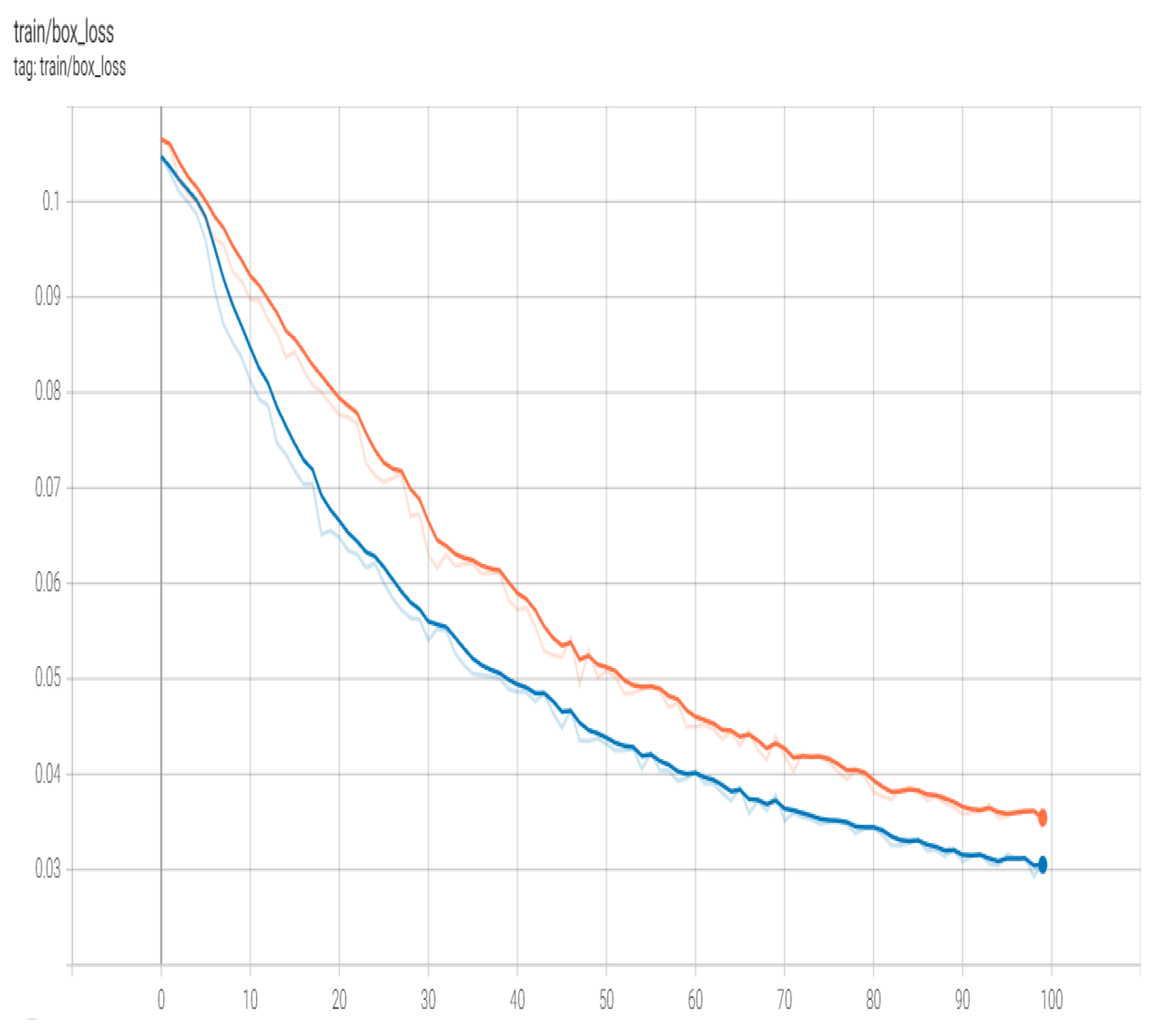
  • box_loss—First, we have box loss, which is the bounding box regression loss (Mean Squared Error).
  • obj_loss—Object loss (or obj loss) is the degree to which one doubts the presence of an object.
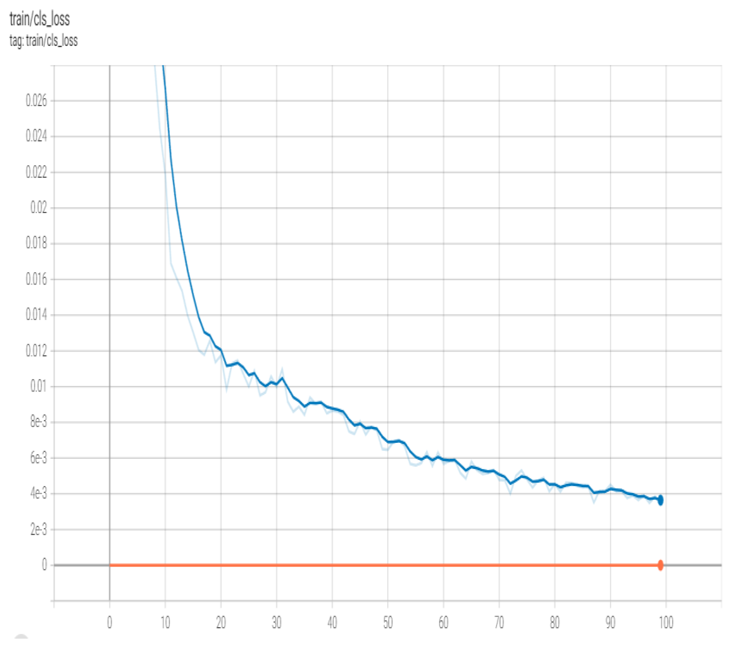
  • cls_loss—The classification loss, or cls loss, is the third variable (Cross-Entropy).

Figure 5 shows training cls_loss of the proposed model and training box_loss has been shown in Figure 6 with respective to existing model and proposed model. Red colour curve represents existing model & Blue colour curve represents proposed model for all figures.

4.3. Classification Measure

The following parameters help better understand and analyze the model and its performance.

a. 

Accuracy: It defines the percentage of accurate forecasts as all forecasts provided. The formula gives it:

$$Accuracy=\frac{TP+TN}{TP+TN+FP+FP}=\frac{Correct predictions}{Total predictions}$$

(11)

b. 

Precision: It may be defined as the fraction of valid positive classes relative to the total number of anticipated actual positive classes. It is calculated as:

$$Precision=\frac{TP}{TP+FP}=\frac{Predictions actually positive}{Total predicted positive}$$

(12)

c. 

Recall (TPR, Sensitivity): It is calculated as:

$$Recall=\frac{TP}{TP+TN}=\frac{Predictions actually positive}{Total actual positive}$$

(13)

Table 2. Classification Measure.

Optimizer	Images	Precision	Recall	[email protected]	[email protected]:.95
SGD Optimizer	1499	0.857	0.816	0.055	0.019
Bayesian Optimizer	1499	0.935	0.830	0.704	0.349
LwF Optimizer	1499	0.988	0.908	0.819	0.569

demonstrates the classification measure for different optimizers (SGD, Bayesian, and LwF optimizers) with the YOLO model in classifying the weather conditions.

Figure 7 and Figure 8 shows precision and recall, respectively, as below.

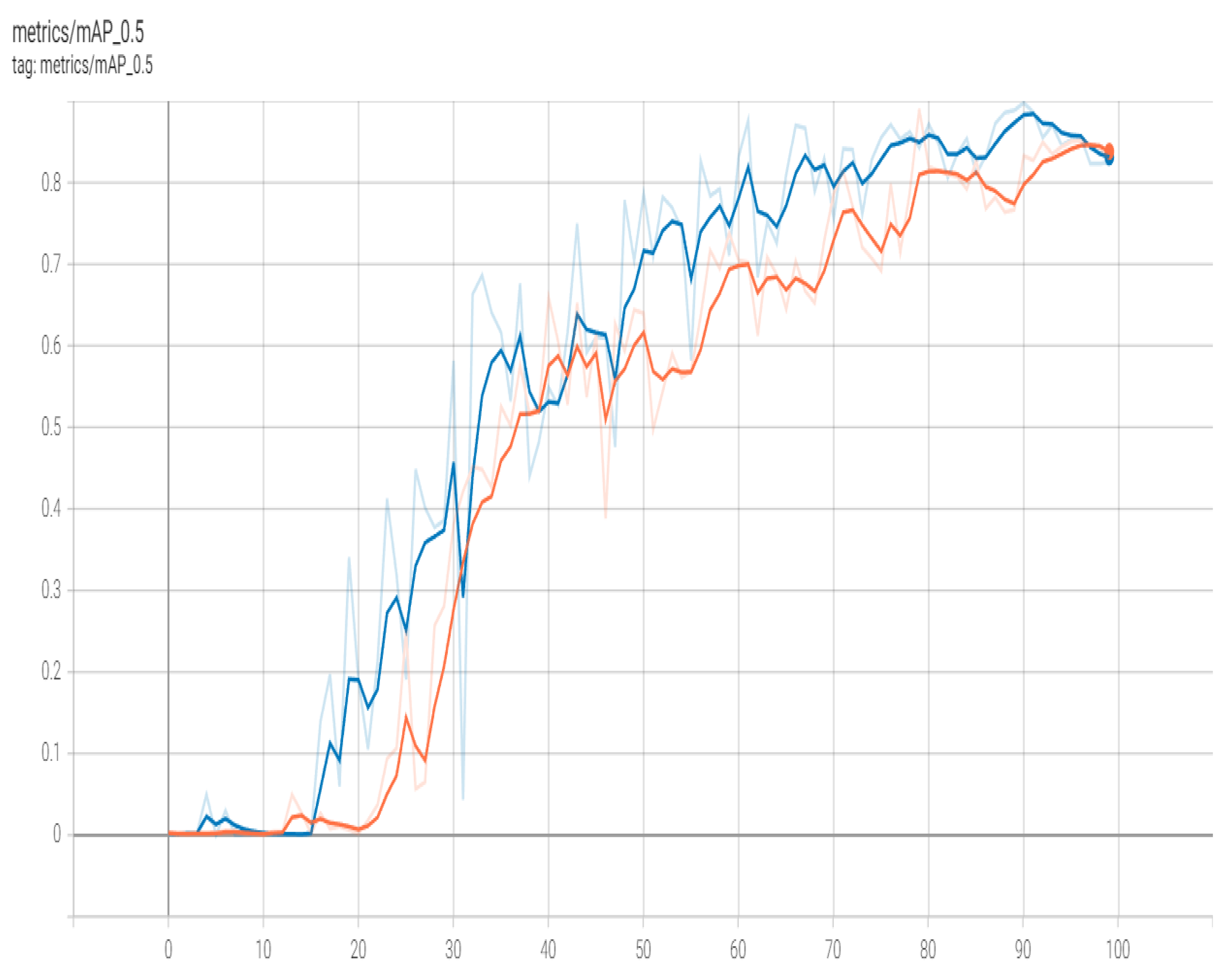
• Object detection accuracy is commonly measured using AP (average precision). The area under the aforementioned precision–recall curve is one way to quantify this.

It is calculated using the formula:

$$AP={\int }_0^{1}p\left(r\right)dr$$

(14)

Figure 9 illustrates mAP_0.95, and Figure 10 illustrates mAP_0.5.

• Training Loss evaluates how well a deep learning model fits the training data by measuring the model’s error on the training set. Figure 11 shows train obj_loss.

Figure 12 depicts the confusion matrix, and Figure 13 shows the confusion matrix for the weather classification chosen.

Table 3. Results comparison.

S. No.	Paper	Methods	Accuracy (%)
1	Wang et al. [16]	SVM	90
2	Hongwei et al. [17]	GA	75
3	Zhang et al. [19]	multiple kernel learning	59.44
4	Lu et al. [21]	CNN	91.4
5	Li et al. [22]	Generative adversarial networks (GAN)	98.09
6	Wang et al. [24]	ResNet and DenseNet	72.25
7	Bai et al. [26]	Multimodal Information Fusion	98.46
8	Proposed Model	Yolo Model with LwF	99.19%

demonstrates the results of various methods, and the proposed method regarding accuracy performance metrics. It has been observed that the proposed model gained higher accuracy than existing models.

5. Conclusions

In this study, we develop a modified Yolo5 model with integration of Learning-without-forgetting (LwF) that can classify weather images with little processing power. This model enhances driving scenarios needed for weather picture categorization while assuring accuracy, and proposed model has the reasoning power equivalent to deep CNN, and it helps in minimizing road accidents. As part of our ongoing commitment to improving people’s quality of life via research, we plan to continue to enhance CNN’s target feature extraction capability, boost accuracy, and cut down on traffic accidents. The proposed model gained the accuracy level of 99.19%. The proposed model gained a 0.988 precision value, a 0.908 recall value, a 0.819 [email protected] value, and a 0.569 [email protected]:.95, respectively. The dataset consists of various weather classifications i.e., “Cloud”, “Fog”, “Rain”, “Snow”, etc. The performance metric depicts the enhanced and improved performance level of the proposed model.

Based on the findings of this model, the dataset might be increased to enable better weather categorization in the future, acquire more valuable features, and boost the model’s capacity for learning. Accurately recognizing weather types is the foundation for estimating rain amounts.

References

1. Momma, E.; Ono, T.; Ishii, H. Rock classification by types and degrees of weathering. In Proceedings of the 2006 SICE-ICASE International Joint Conference, Busan, Republic of Korea, 18–21 October 2006; pp. 149–156. [Google Scholar] [CrossRef]
2. Yusoff, I.N.; Mohamad Ismail, M.A.; Tobe, H.; Date, K.; Yokota, Y. Quantitative granitic weathering assessment for rock mass classification optimization of tunnel face using image analysis technique. Ain Shams Eng. J. 2023, 14, 101814. [Google Scholar] [CrossRef]
3. Zhang, H.; Xu, J.; Zou, S. A classification learning system based on multi-objective GA and microthermal weather forecast. In Proceedings of the 2nd International Conference on Digital Manufacturing and Automation, ICDMA 2011, Zhangjiajie, China, 5–7 August 2011; pp. 301–304. [Google Scholar] [CrossRef]
4. Solis-Aulestia, M.; Pineda, I.; Piispa, E.J.; Williams, S.L. Evaluation of Evapotranspiration Classification Using Self-Organizing Maps and Weather Research and Forecasting Variables. In Proceedings of the International Geoscience and Remote Sensing Symposium (IGARSS), Kuala Lumpur, Malaysia, 17–22 July 2022; pp. 3195–3198. [Google Scholar] [CrossRef]
5. Vasiliev, O.V.; Boyarenko, E.S.; Galaeva, K.I.; Zyabkin, S.A. Concerning the Issue of Classification of Hazardous Weather Events. In Proceedings of the 19th Technical Scientific Conference on Aviation Dedicated to the Memory of N.E. Zhukovsky, TSCZh 2022, Moscow, Russia, 14–15 April 2022; pp. 76–78. [Google Scholar] [CrossRef]
6. Huang CM, T.; Huang, Y.C.; Huang, K.Y. A hybrid method for one-day ahead hourly forecasting of PV power output. In Proceedings of the 9th IEEE Conference on Industrial Electronics and Applications, ICIEA 2014, Hangzhou, China, 9–11 June 2014; pp. 526–531. [Google Scholar] [CrossRef]
7. Trombe, P.J.; Pinson, P.; Madsen, H. Automatic classification of offshore wind regimes with weather radar observations. IEEE J. Sel. Top. Appl. Earth Obs. Remote Sens. 2014, 7, 116–125. [Google Scholar] [CrossRef] [Green Version]
8. Zhang, Z.; Ma, H. Multi-class weather classification on single images. In Proceedings of the 2015 IEEE International Conference on Image Processing (ICIP), Quebec City, QC, Canada, 27–30 September 2015; pp. 4396–4400. [Google Scholar]
9. Mohapatra, A.G.; Lenka, S.K. Neural Network Pattern Classification and Weather Dependent Fuzzy Logic Model for Irrigation Control in WSN Based Precision Agriculture. Phys. Procedia 2016, 78, 499–506. [Google Scholar] [CrossRef] [Green Version]
10. Roberto, N.; Baldini, L.; Adirosi, E.; Lischi, S.; Lupidi, A.; Cuccoli, F.; Barcaroli, E.; Facheris, L. Test and validation of particle classification based on meteorological model and weather radar simulator. In Proceedings of the 13th European Radar Conference, EuRAD 2016, London, UK, 5–7 October 2016; pp. 201–204. [Google Scholar]
11. Lin, D.; Lu, C.; Huang, H.; Jia, J. RSCM: Region Selection and Concurrency Model for Multi-Class Weather Recognition. IEEE Trans. Image Process. 2017, 26, 4154–4167. [Google Scholar] [CrossRef] [PubMed]
12. Lu, C.; Lin, D.; Jia, J.; Tang, C.K. Two-Class Weather Classification. IEEE Trans. Pattern Anal. Mach. Intell. 2017, 39, 2510–2524. [Google Scholar] [CrossRef] [PubMed] [Green Version]
13. Pandey, A.K.; Agrawal, C.P.; Agrawal, M. A hadoop based weather prediction model for classification of weather data. In Proceedings of the 2nd IEEE International Conference on Electrical, Computer and Communication Technologies, ICECCT 2017, Coimbatore, India, 22–24 February 2017; pp. 1–5. [Google Scholar] [CrossRef]
14. Kunjumon, C.; Nair, S.S.; Deepa Rajan, S.; Padma Suresh, L.; Preetha, S.L. Survey on Weather Forecasting Using Data Mining. In Proceedings of the IEEE Conference on Emerging Devices and Smart Systems, ICEDSS 2018, Tiruchengode, India, 2–3 March 2018; pp. 262–264. [Google Scholar] [CrossRef]
15. Peng, X.; Fan, W.; Yang, F.; Che, J.; Wang, B. A short-term wind power prediction approach based on the dynamic classification of the weather types of wind farms. In Proceedings of the CIEEC 2017—Proceedings of 2017 China International Electrical and Energy Conference, Beijing, China, 25–27 October 2017; pp. 612–615. [Google Scholar] [CrossRef]
16. Wang, S.; Li, Y.; Feng, S. A Multitask Learning Approach for Weather Classification on Railway Transportation. In Proceedings of the International Conference on Intelligent Rail Transportation, ICIRT 2018, Singapore, 12–14 December 2018. [Google Scholar] [CrossRef]
17. Hongwei, X.; Fang, F.; Liu, J. Weather-Classification-MARS-Based Photovoltaic Power Forecasting for Energy Imbalance Market. IEEE Trans. Ind. Electron. 2019, 66, 8692–8702. [Google Scholar] [CrossRef]
18. Shi, J.; Lee, W.J.; Liu, Y.; Yang, Y.; Wang, P. Forecasting power output of photovoltaic systems based on weather classification and support vector machines. IEEE Trans. Ind. Appl. 2012, 48, 1064–1069. [Google Scholar] [CrossRef]
19. Zhang, Z.; Jin, Y.; Li, Y.; Lin, Z.; Wang, S. Imbalanced adversarial learning for weather image generation and classification. In Proceedings of the 14th IEEE International Conference on Signal Processing (ICSP), Beijing, China, 12–16 August 2018; pp. 1093–1097. [Google Scholar] [CrossRef]
20. Wang, Y.; Li, Y.X. Research on Multi-class Weather Classification Algorithm Based on Multi-model Fusion. In Proceedings of 4th IEEE Information Technology, Networking, Electronic and Automation Control Conference, ITNEC 2020, Chongqing, China, 12–14 June 2020; pp. 2251–2255. [Google Scholar] [CrossRef]
21. Lu, Z.; Ding, X.; Ren, Y.; Sun, X. Multi-Classification of Rainfall Weather Based on Deep Learning-Mod. In Proceedings of the 2020 39th Chinese Control Conference (CCC), Shenyang, China, 27–29 July 2020; pp. 6374–6379. [Google Scholar] [CrossRef]
22. Li, L.W.; Chou, K.L.; Fu, R.H. Deep learning-based weather image recognition. In Proceedings of the 2018 International Symposium on Computer, Consumer and Control (IS3C), Taichung, Taiwan, 6–8 December 2018; pp. 384–387. [Google Scholar] [CrossRef]
23. Zhang, H.; Zhao, X.; Zou, S. Neuron classification algorithm and megathermal weather forecast. In Proceedings of the 2011 3rd International Workshop on Intelligent Systems and Applications, Wuhan, China, 28–29 May 2011; pp. 24–27. [Google Scholar] [CrossRef]
24. Wang, Z.W.; Zhang, C.L.; Su, C.; Cheng, C.L. On the modeling of atmospheric visibility classification forecast with nonlinear support vector machine. In Proceedings of the 5th International Conference on Natural Computation, ICNC 2009, Tianjian, China, 14–16 August 2009; pp. 240–244. [Google Scholar] [CrossRef]
25. Bai, C.; Zhao, D.; Zhang, M.; Zhang, J. Multimodal Information Fusion for Weather Systems and Clouds Identification from Satellite Images. IEEE J. Sel. Top. Appl. Earth Obs. Remote Sens. 2022, 15, 7333–7345. [Google Scholar] [CrossRef]
26. Alem, S.; Duan, L.; Zhang, Z.; Cao, X. Hierarchical Multimodal Fusion for Ground-Based Cloud Classification in Weather Station Networks. IEEE Access 2019, 7, 85688–85695. [Google Scholar] [CrossRef]
27. Deng, X.; Ye, A.; Zhong, J.; Xu, D.; Yang, W.; Song, Z.; Zhang, Z.; Guo, J.; Wang, T.; Tian, Y.; et al. Bagging–XGBoost algorithm based extreme weather identification and short-term load forecasting model. Energy Rep. 2022, 8, 8661–8674. [Google Scholar] [CrossRef]
28. Fang, C.; Lv, C.; Cai, F.; Liu, H.; Wang, J.; Shuai, M. Weather Classification for Outdoor Power Monitoring based on Improved SqueezeNet. In Proceedings of the 5th International Conference on Information Science, Computer Technology and Transportation, ISCTT 2020, Shenyang, China, 13–15 November 2020; pp. 11–15. [Google Scholar] [CrossRef]
29. Yang, F.; Watson, P.; Koukoula, M.; Anagnostou, E.N. Enhancing Weather-Related Power Outage Prediction by Event Severity Classification. IEEE Access 2020, 8, 60029–60042. [Google Scholar] [CrossRef]
30. Dalal, S.; Goel, P.; Onyema, E.M.; Alharbi, A.; Mahmoud, A.; Algarni, M.A.; Awal, H. Application of Machine Learning for Cardiovascular Disease Risk Prediction. Comput. Intell. Neurosci. 2023, 9418666. [Google Scholar] [CrossRef]
31. Dalal, S.; Onyema, E.M.; Malik, A. Hybrid XGBoost model with hyperparameter tuning for prediction of liver disease with better accuracy. World J. Gastroenterol. 2022, 28, 6551–6563. [Google Scholar] [CrossRef] [PubMed]
32. Huang, Y.; Jin, Y.; Li, Y.; Lin, Z. Towards Imbalanced Image Classification: A Generative Adversarial Network Ensemble Learning Method. IEEE Access 2020, 8, 88399–88409. [Google Scholar] [CrossRef]
33. Goswami, S. Towards Effective Categorization of Weather Images using Deep Convolutional Architecture. In Proceedings of the 2020 International Conference on Industry 4.0 Technology, I4Tech 2020, Pune, India, 13–15 February 2020; pp. 76–79. [Google Scholar] [CrossRef]
34. Baig, H.A.; Arshad, A.; Raza, A. Two class weather classification with bagging technique. In Proceedings of the 4th International Conference on Innovative Computing, ICIC 2021, Lahore, Pakistan, 9–10 November 2021; pp. 21–26. [Google Scholar] [CrossRef]
35. Stepchenko, A.M. Land-Use Classification Using Convolutional Neural Networks. Autom. Control. Comput. Sci. 2021, 55, 358–367. [Google Scholar] [CrossRef]
36. Gikunda, P.; Jouandeau, N. Homogeneous Transfer Active Learning for Time Series Classification. In Proceedings of the 20th IEEE International Conference on Machine Learning and Applications, ICMLA 2021, Pasadena, CA, USA, 13–16 December 2021; pp. 778–784. [Google Scholar] [CrossRef]
37. Dalal, S.; Onyema, E.M.; Kumar, P.; Maryann, D.C.; Roselyn, A.O.; Obichili, M.I. A hybrid machine learning model for timely prediction of breast cancer. Int. J. Model. Simul. Sci. Comput. 2022, 2023, 410234. [Google Scholar] [CrossRef]
38. Zhao, X.; Wu, C. Weather Classification Based on Convolutional Neural Networks. In Proceedings of the 2021 International Conference on Wireless Communications and Smart Grid, ICWCSG 2021, Hangzhou, China, 13–15 August 2021; pp. 293–296. [Google Scholar] [CrossRef]
39. Shankarnarayan, V.K.; Ramakrishna, H. Comparative study of three stochastic future weather forecast approaches: A case study. J. Inf. Technol. Data Manag. 2021, 3, 3–12. [Google Scholar] [CrossRef]
40. Malik, M.; Nandal, R.; Dalal, S.; Jalglan, V.; Le, D.-N. Deriving Driver Behavioral Pattern Analysis and Performance Using Neural Network Approaches. Intell. Autom. Soft Comput. 2022, 32, 87–99. [Google Scholar] [CrossRef]
41. Purwandari, K.; Sigalingging, J.W.; Cenggoro, T.W.; Pardamean, B. Multi-class Weather Forecasting from Twitter Using Machine Learning Aprroaches. Procedia Comput. Sci. 2021, 179, 47–54. [Google Scholar] [CrossRef]
42. Dash, R.; Dash, D.K.; Biswal, G. Classification of crop based on macronutrients and weather data using machine learning techniques. Results Eng. 2021, 9, 100203. [Google Scholar] [CrossRef]
43. Tian, M.; Chen, X.; Zhang, H.; Zhang, P.; Cao, K.; Wang, R. Weather classification method based on spiking neural network. In Proceedings of the 2021 International Conference on Digital Society and Intelligent Systems, DSInS 2021, Chengdu, China, 3–4 December 2021; pp. 134–137. [Google Scholar] [CrossRef]
44. Cheng, Q.; Wu, Z.; Min, J. Foggy Weather Monitoring Method Based on Improved Deep Residual Shrinkage Network and Radio Signal. In Proceedings of the 3rd International Conference on Geology, Mapping and Remote Sensing, ICGMRS 2022, Zhoushan, China, 22–24 April 2022; pp. 495–499. [Google Scholar] [CrossRef]
45. Abu-Abdoun, D.I.; Al-Shihabi, S. Weather Conditions and COVID-19 Cases: Insights from the GCC Countries. Intell. Syst. Appl. 2022, 200093. [Google Scholar] [CrossRef]
46. Ali, E.M.; Ahmed, M.M. Employment of instrumented vehicles to identify real-time snowy weather conditions on freeways using supervised machine learning techniques—A naturalistic driving study. IATSS Res. 2022, 46, 525–536. [Google Scholar] [CrossRef]
47. Malik, M.; Nandal, R.; Dalal, S.; Maan, U.; Le, D.-N. An efficient driver behavioral pattern analysis based on fuzzy logical feature selection and classification in big data analysis. J. Intell. Fuzzy Syst. 2022, 43, 3283–3292. [Google Scholar] [CrossRef]
48. Chen, B.; Wang, Y.; Huang, J.; Zhao, L.; Chen, R.; Song, Z.; Hu, J. Estimation of near-surface ozone concentration and analysis of main weather situation in China based on machine learning model and Himawari-8 TOAR data. Sci. Total. Environ. 2023, 864, 160928. [Google Scholar] [CrossRef]
Figure 1. Multitask learning methods. (a) Fine Tuning. (b) Original model. (c) Feature extraction. (d) Joint training.
Sustainability 15 06070 g001
Figure 2. Learning without Forgetting (LwF).
Sustainability 15 06070 g002
Figure 3. Flowchart of LwF.
Sustainability 15 06070 g003
Figure 4. Multiple object detection mechanism using YOLO.
Sustainability 15 06070 g004
Figure 5. Training Cls_loss. Red colour curve represents existing model & Blue colour curve represents proposed model.
Sustainability 15 06070 g005
Figure 6. Training box_loss. Red colour curve represents existing model & Blue colour curve represents proposed model.
Sustainability 15 06070 g006
Figure 7. Precision. Red colour curve represents existing model & Blue colour curve represents proposed model.
Sustainability 15 06070 g007
Figure 8. Recall. Red colour curve represents existing model & Blue colour curve represents proposed model.
Sustainability 15 06070 g008
Figure 9. mAP_0.95. Red colour curve represents existing model & Blue colour curve represents proposed model.
Sustainability 15 06070 g009
Figure 10. mAP_0.5. Red colour curve represents existing model & Blue colour curve represents proposed model.
Sustainability 15 06070 g010
Figure 11. Train obj_loss. Red colour curve represents existing model & Blue colour curve represents proposed model.
Sustainability 15 06070 g011
Figure 12. Confusion matrix.
Sustainability 15 06070 g012
Figure 13. Confusion matrix for weather.
Sustainability 15 06070 g013