An Empirical Approach to Integrating Climate Reputational Risk in Long-Term Scenario Analysis

Abstract

We propose an empirical approach to estimate the impact of climate transition risk on corporate revenues that specifically accounts for reputational risk. We employ the information on disclosed Scope 3 emissions to proxy companies’ carbon footprint along the value chain. A threshold regression is employed to identify the emission level above which reputational risk impacts revenues, and we link this impact to a climate policy stringency indicator. We estimate the threshold regression on a sample of companies within the European Union (EU), and find the threshold at around the 70th percentile of the Scope 3 emissions distribution. We find that companies with Scope 3 emissions beyond the threshold experienced substantially lower revenue growth as climate policies have become more stringent, compared to other companies.

1. Introduction

The climate is an influential driver of global economic and social development [1]. Climate change, and a temperature increase above 2° compared to pre-industrial levels in particular, could have devastating consequences on the environment and biodiversity [2], human health [3], and migration [4], in addition to increased frequency and severity of extreme weather events [5]. In 2015, 195 countries signed the Paris Agreement, but progress on keeping the temperature rise below 2° has been too slow, urging more decisive climate action to prevent far higher costs in the next decades [6].

Climate action, however, does come at a price. This is undoubtedly the cost of investment in low-emission and climate-resilient energy infrastructure and reforming policies to improve resource allocation [7], which is mainly sustained through public expenditure and adds to the cost of stranded asset replacement and investment in low-carbon production technologies to be paid for by the private sector. It must be added that climate policies themselves will be a source of indirect costs for the business sector, especially for some industries. For instance, transition pathways imply a high carbon price and high fossil energy prices, translating into higher operative expenses for companies in carbon-intensive industries.

For this reason, climate risk is commonly understood and assessed referring to its dual nature: physical and transition risk. Physical risk emerges due to chronic changes in temperature and precipitation levels that threaten the economy and, in particular, the agricultural sector [8,9,10,11,12,13,14,15], as well as the increased frequency and intensity of extreme events, such as flash floods and river floods [16], wildfires [17], and coastal flooding [18] that could damage production assets. Physical risk exposure is expected to increase significantly in the absence of actions to limit global warming, but its economic consequences are expected to become severe in the long run. Transition risk, in contrast, represents the risk resulting from the implementation of stringent climate policies, which would prevent the long-term damages of global warming but generate a cost to be paid in the short term [19]. Not surprisingly, the trade-off between physical and transition risks has become a key issue in climate risk assessment, as the evidence on the use of the Network for Greening the Financial System (NGFS) scenarios [20] seems to suggest.

The extent to which transition risk exposure affects the financial and economic values of companies has been the object of an increasing number of studies. Many of these studies focused on the financial effects, trying to understand how such risk is capitalized on in stock market prices. Among others, ref. [21] provided general evidence that stock markets react negatively to transition shocks and browner companies are more heavily penalized than their greener counterparts. One paper [22] looked at the behavior of financial operators in relation to the Paris Agreement and found that stock markets have rewarded low-carbon indices and penalized carbon-intensive ones. More specifically, ref. [23] found that carbon-intensive firms pay a higher stock market premium not explained by other risk factors, while [24] found that the cost of option protection against downside tail risks is larger for firms with more carbon-intensive business models. Another paper [25] investigated the EU stock market and found the presence of a negative green premium, i.e., lower stock market returns for green and transparent companies, suggesting that investors are willing to accept lower returns from less climate-risky companies. Another paper [26] looked more specifically at a sample of companies covered by the EU ETS (European Trading Scheme) regulation and found more heterogeneous results, yet ones that suggested the pricing of transition risk in stock markets.

There are three primary drawbacks related to the assessment of transition risk impact on the financial value of companies. The first is that the risk transmission channel is not always clear. Transition risk may impact the company’s balance sheet and, as a consequence, its stock market performance in multiple ways, stemming from the increased cost of operations to the increased capital expenditure required for decarbonization and lower returns due to market and reputational risk [27]. The second is that the proxy used for transition risk exposure is the level of Scope 1 emissions. Hence, only the emissions directly produced by the company in its operations are considered. This approach inevitably excludes the transition risk related to the company’s energy mix (Scope 2 emissions) and its value chain (Scope 3 emissions). The third is that the approaches are backward-looking because they build the statistical models on past observations. A more stringent climate policy, instead, implies changes that have not been experienced so far and for which it is difficult to understand how markets may respond based on past observation.

Climate scenario analysis (CSA) represents a solution to these drawbacks, and for this reason, TCFD recommends it, especially to large companies in highly exposed industries, for their mandatory and voluntary disclosure of climate-related risks and opportunities. A recent joint report of the Financial Stability Board and the Network for Greening the Financial System investigated the use of scenario analysis among financial institutions [28]: quite unsurprisingly, 53 institutions from 36 jurisdictions had already conducted or were conducting similar exercises, testifying to the relevance that this tool is gaining in the scientific and institutional communities. More interestingly, the report suggests that the main reason for conducting CSA is to assess how climate risk could impact financial stability (the macroprudential reason). Next comes the need to develop climate scenario analysis capabilities within the organization, showing that the scope of CSA falls not only in the interest of financial authorities but also financial institutions willing to assess their counterpart’s exposure to climate-related risks.

The structure of a CSA is rather complex when it comes to measuring asset-level physical risk exposure and expected damages on assets. Still, it is relatively straightforward concerning the transition risk. Revenues are directly or indirectly related to the gross domestic product, whose projections change across scenarios. Operating expenses (OpEx) are projected to change according to carbon and energy prices. A higher carbon price resulting from more stringent climate policies in a 1.5/2° scenario will result in higher OpEx because of the higher cost the company has to pay to guarantee business continuity. The expected OpEx impact depends on the company’s exposure: the higher the company’s greenhouse gas (GHG) emissions, the higher the impact. The mechanism is nearly the same for the energy prices, but the impact depends on the company’s energy mix. A more balanced energy mix toward fossil fuels implies higher future OpEx in a Paris-aligned scenario in which relatively high fossil fuel prices discourage their use. Capital expenditures (CapEx) are also expected to increase if the company decides to invest in decarbonizing its production or in changing the energy mix to reduce its balance sheet exposure to transition risk.

Carbon and energy prices, being associated with direct (Scope 1) and indirect (Scope 2) emissions, respectively, cover a significant share of climate risk exposure for many companies, but do not account for the reputational risk related to changes in consumer preferences [27]. This risk is instead associated with Scope 3 emissions [29,30,31], since they are produced along the value chain and hence represent the bulk of corporate emissions. In a Paris-aligned scenario, companies with higher Scope 3 emissions will be penalized by consumers with a downshift in demand for carbon-intensive products.

In the CSA application performed by the European Central Bank [30], for instance, a value added tax (VAT) rate increase is assumed for companies with high Scope 3 emissions. Although the VAT rate is not a typical climate policy instrument, because it is not going to be used to influence customers’ decisions in reality, it hypothetically delivers, using standard econometric methods, the desired effect in the CSA framework: companies with high Scope 3 emissions level will experience a decrease in market share and, hence, revenues. To the best of the authors’ knowledge, the ECB approach is the first to incorporate reputational risk in a CSA framework, as similar CSA applications do not include reputational risk among their transmission channels. For instance, the Bank of England framework considers only disruptive technological advances and the government’s climate policies among transition risk channels [32]. The Netherlands Central Bank uses a very similar approach, with a more pronounced focus on energy transition [33]. Likewise, reputational risk is not considered in the European Systemic Risk Board framework [34] as well as in the Banque de France application [35]. Similarly to institutional CSA exercises, academic attention on climate reputational risk in the context of CSA has also been limited. For instance, the study by [36] focuses mainly on the implications for companies of technology and policy shocks in response to climate change. Considerations about reputational risk are not included in the work of [37], an essential reference in climate scenario analysis. Certainly, the field is evolving rapidly and much remains to be done to understand climate risk transition channels [38].

However, climate reputational risk has been largely investigated in the scientific literature. Ref. [39] explore the connection between sustainability reporting and reputational risk, suggesting the former may serve as a driver for the latter. Even though their analysis is not strictly related to climate reputational risk, this hypothesis may well explain the increasing number of companies reporting climate performance, especially after the Paris Agreement [40]. Studies reporting on empirical evidence about climate transition risk exposure and impacts on companies use policy and technology change events. For instance, ref. [41] found evidence of stock value changes of largest polluting companies after climate-related events that attracted media attention, such as the Paris Agreement and Greta Thunberg’s speech at the United Nations. Another paper [42] studied the financial impacts for US companies in the Oil and Gas sector from Trump’s announcement of the Paris Agreement withdrawal. Both of these studies measure climate reputational risk indirectly, hence in relation to a climate-relevant event, and do not link the risk to any company-level measure of climate performance. The paper by [31] is the only empirical study, to the best of the authors’ knowledge, that attempts to link reputational risk to climate performance. They employ a standard econometric model and a sample of US firms to investigate whether sources of carbon emissions are linked to firms’ reputational risk, as measured by a score provided by RepRisk, an ESG data provider. They find that Scope 3 emissions only (i.e., not other sources of emissions) are positively associated with climate reputational risk, and interpret this result as investors demanding a higher carbon premium for their exposure to climate risks associated with increasing Scope 3 emissions. They do not, however, investigate the effect of climate reputational risk on firms’ revenues.

Notwithstanding the increasing interest in climate transition risk, extant literature has not yet produced evidence of the economic and financial impacts of directly measured reputational risk. We fill this gap, and hence extend the aforementioned literature, by proposing a novel methodological approach to estimate the relationship between Scope 3 emissions, the most reliable proxy for reputational risk [31], and revenue change, using historical data. The framework we propose builds on a regression of revenues growth (target variable) on Scope 3 emissions (explanatory variable), accounting for standard revenue growth determinants. Our approach departs from the standard linear regression model, adopted by [30,31], in two ways. First, we assume that the main impact of Scope 3 emissions on revenue shows up after a critical level of Scope 3 only. We believe that this assumption better reflects reality, where not all firms are effectively at risk, but only those with the highest carbon footprints. Second, the impact on revenue growth depends on how stringent climate policies have been and will be in the future.

To deliver this non-linear effect, our proposed methodology leverages the threshold regression model, with interaction terms, as seen in [43]. This model is used to estimate the level of Scope 3 emissions above which the main negative effect on revenues shows up. The advantage of [43]’s approach is that it allows the threshold parameter to be estimated from the data alongside the other model parameters, avoiding subjective assumptions about the threshold level, which may be informed by external information. The interaction term allows the estimated effect to vary with the policy stringency parameter which, in our case, is the carbon price, as measured by the European Trading Scheme (ETS) price. In short, the ETS mechanism, based on cap-and-trade, defines the rule for the emission allowances (cap) to be distributed across industries and firms, and lets companies exchange the allowances in excess (trade). The cap (the number of allowances) is periodically redefined and diminished to make the traded part progressively more relevant while reducing overall emissions. As the price is directly related to the overall number of allowances (the climate policy instrument), it indirectly reflects the climate policy stringency.

The threshold regression model is estimated on an unbalanced panel of companies within the EU, using economic, financial, and Scope 3 data from the Refinitiv, Organisation for Economic Co-operation and Development (OECD), and European Commission databases. The overall sample includes 693 companies observed for 10 years, for a total of 3320 data points. The sample is limited only to those companies for which Scope 3 data are available, which is a small number, admittedly. This is a clear limitation, because it is quite possible that we are picking the highest polluting companies, and the interpretation of the results and the scope of conclusions should be limited accordingly. However, the sample selection involves the explanatory and not the target variable, and this allows us to exclude estimation bias due to sample selection [44].

This paper contributes to two strands of empirical literature. On the one hand, it provides novel evidence of the economic and financial impact of transition risk for companies, suggesting that Scope 3 emissions are a good predictor of revenue growth. We deem this contribution relevant because many existing works so far focused on Scope 1 or Scope 2 (or both) emissions, and neglected Scope 3. While this choice was arguably justified by the sample size reduction due to the little information on Scope 3 (as Scope 1 and Scope 2 data are relatively more available), we show that it is relevant as well, and should be considered in empirical analyses. On the other hand, our paper contributes to the growing number of institutional works relying on CSA, by providing a novel framework for the consideration of companies’ reputational risk.

The paper is structured as follows. Section 2 describes in detail the threshold regression model and the data used for its estimation. Section 3 discusses the results of the empirical analysis, and Section 4 concludes the paper.

2. Econometric Methodology and Data Description

This section starts by illustrating the form, variables, and estimation method of the econometric model used to capture companies’ exposure to climate reputational risk. We then conduct a data exploration analysis, which anticipates the estimation results discussed in the next section.

2.1. A Threshold Regression Approach to Model Climate Reputational Risk

The impact of climate reputational risk on corporate revenues is investigated by means of econometric techniques. Specifically, we employ a threshold regression model which takes the following form

$$\begin{array}{cc}\hfill \%\Delta Revenu{e}_{i,t}=& {\beta }_0+{\beta }_1\%\Delta Revenu{e}_{i,t-1}+{\beta }_2\%\Delta TotalAsset{s}_{i,t}\hfill \\ & +{\beta }_{3}log\left(PriceEU{A}_{t}Scope{3}_{i,t}\right)+{\beta }_4{D}_{i,t}+{\beta }_5{D}_{i,t}log\left(PriceEU{A}_{t}Scope{3}_{i,t}\right)\hfill \\ & +{\beta }_{6}Countr{y}_i+{\beta }_{7}Siz{e}_i+{\beta }_{8}Industr{y}_i+{\beta }_{9}VA{T}_{i,t}+{\beta }_{10}t+{\epsilon }_{i,t},\hfill \end{array}$$

(1)

for $i=1,\cdots ,n$ and $t=1,\cdots ,T$, and where i and t are index firms and years, respectively. We are in the case $T<n$, and the first time lag of the dependent variable is among the regressors. Hence, we are dealing with a dynamic threshold regression model for panel data. We assume no individual effects in the error term ${\epsilon }_{i,t}$, as we believe these are mostly captured by the categorical regressors included in the model ($Country$, $Size$, and $Industry$). We further assume cross-sectionally independent observations, and ${\epsilon }_{i,t}$ to have mean zero and to be normally distributed, homoskedastic, and mean independent of all regressors (which is a type of exogeneity assumption on these).

We define the yearly percentage changes of revenues and total assets as $\%\Delta Revenu{e}_{i,t}=\frac{Revenu{e}_{i,t}-Revenu{e}_{i,t-1}}{Revenu{e}_{i,t-1}}100$ and $\%\Delta TotalAsset{s}_{i,t}=\frac{TotalAsset{s}_{i,t}-TotalAsset{s}_{i,t-1}}{TotalAsset{s}_{i,t-1}}100$, respectively.

The choice of regressors is partly inspired by [30], who perform a climate stress-test exercise to evaluate the impact of climate-related risks on firms’ main balance sheet indicators, including revenues. The covariates proposed by [30] are discussed in what follows. The first lag of the dependent variable, as well as a linear and deterministic time trend t, are both supposed to capture time-related features of the dependent variable (serial correlation and trending behavior, respectively). The percentage changes of total assets $\%\Delta TotalAsset{s}_{i,t}$, are assumed to drive $\%\Delta Revenue{s}_{i,t}$ in their same direction. For example, a decrease in total assets due to the loss of a tangible asset comports with a reduction also in revenues. The VAT rate ($VAT$), which varies little across countries and (for some of those) also little over time, is included in the equation since tax increments could decrease firms’ revenues, due to a drop in the demand for products subject to a higher taxation. The categorical regressors, already mentioned above, are defined as follows. The variable $Country$ represents the country of headquarters of a firm, and varies across the 27 EU Member States. The size of a company is determined by the number of its employees. According to the guidelines drawn by [45], we distinguish four size categories:

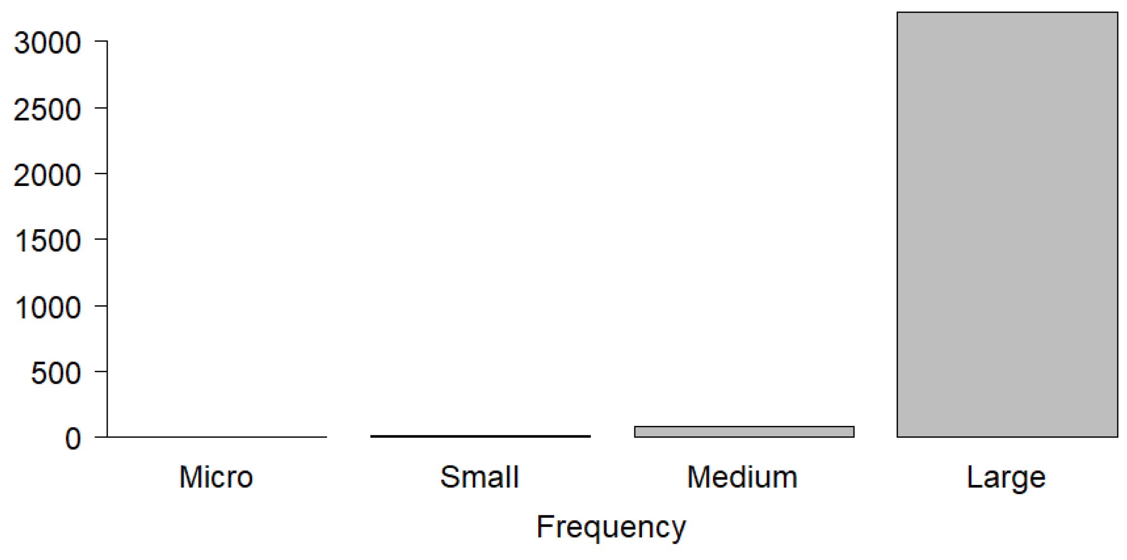
• Micro, with ≤10 employees
• Small, with <50 employees
• Medium, with <250 employees
• Large, with ≥250 employees.

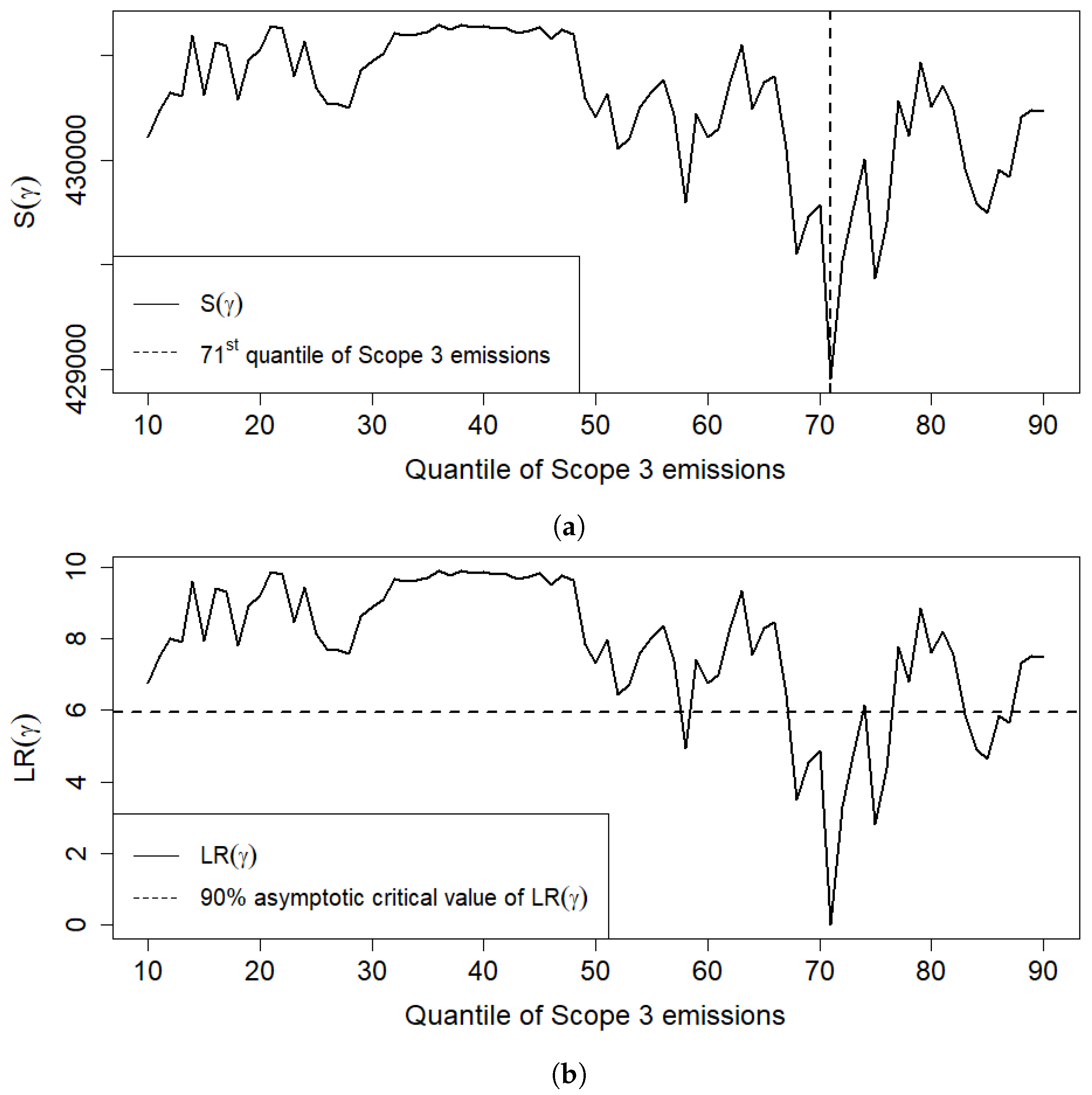
Contrary to the number of employees, $Size$ is a variable that does not change over time, as shown by the indeces in Equation (1). We, therefore, assume that the size of a company is equal, through time, to its latest observed category.(There were no companies that changed country or headquarters, in our sample.) Finally, the industry sectors correspond to level 2 of the Nomenclature of Economic Activities (NACE) Rev. 2 classification, which is made of 88 divisions identified by two-digit numerical codes, from 01 to 99 [46].

Going beyond [30], we also include $log\left(PriceEU{A}_{t}Scope{3}_{i,t}\right)$ among the regressors of model (1), for the purpose of capturing climate reputational risk. Scope 3 emissions are all indirect GHG emissions that occur along the value chain of a company, and are measured in tonnes. They represent a company’s carbon footprint and are by far the majority of firms’ total emissions, especially for large companies [30,47]. For this reason, they are of high concern when it comes to climate change, and we employ them, instead of Scope 1 or Scope 2 emissions, for modelling climate reputational risk.

The variable $PriceEU{A}_t$ represents the price of the European Emission Allowances (EUAs) of the EU ETS. The EU ETS is a cap-and-trade program that sets a limit, or “cap”, to the amount of GHGs that can be emitted each year by power plants, industrial factories, and the aviation sector covered by the system [48]. These entities receive or buy emission allowances, which they can trade with one another as needed. Each allowance gives the holder the right to emit one ton of carbon dioxide (CO₂) equivalent. The cap decreases every year, ensuring a fall in total emissions. The price of the EUAs, $PriceEU{A}_t$, is common among all EU Member States (thus, it is not characterized by a cross-sectional variation) and it is measured in EUR/ton of CO₂. Although it is related only to direct emissions of the entities covered by the EU ETS, and not all firms in our sample are among them, we treat it as a proxy for the carbon price. Consequently, by multiplying $PriceEU{A}_t$ by $Scope{3}_{i,t}$ we obtain a proxy for time and firm-specific cost for Scope 3 emissions, which can be interpreted as a climate policy stringency indicator on carbon-intensive goods: the higher $log\left(PriceEU{A}_{t}Scope{3}_{i,t}\right)$, the greater a firm’s exposure to this climate policy indicator.

A summary of the definition of all variables discussed above is provided in

Table A1. Variable definitions. Most of the descriptions correspond to the ones provided by the corresponding data sources.

Variable	Description	Unit of Measure	Source
$\%\Delta Revenu{e}_{i,t}$	Yearly percentage change of the total revenue of a company. Total revenue includes: revenue from goods and services; revenue from financing-related operations; revenue from business-related activities.	%	Refinitiv
$\%\Delta TotalAsset{s}_{i,t}$	Yearly percentage change of total assets reported by a company.	%	Refinitiv
$PriceEU{A}_t$	Price of the European Emission Allowances of the EU Emissions Trading System	€/ton of CO2	Refinitiv
$Scope{3}_{i,t}$	Emissions from contractor-owned vehicles, employee business travel (by rail or air), waste disposal, outsourced activities, emissions from product use by customers, emission from the production of purchased materials, emissions from electricity purchased for resale.	Tonnes	Refinitiv
$VA{T}_{i,t}$	Value Added Tax rate. The VAT is a consumption tax that is applied to nearly all goods and services that are bought and sold for use or consumption in the EU.	%	OECD & European Commission
$Countr{y}_i$	Country of Headquarters, also known as Country of Domicile.		Refinitiv
$Siz{e}_i$	The size of a company is determined (as described in Section 2.1) by the number of full-time employees, as reported, as of the fiscal period end date (we download data about firms’ number of full-time employees).		Refinitiv
$Industr{y}_i$	NACE (for the French term “Nomenclature statistique des Activités Economiques dans la Communauté Européenne”), is the industry standard classification system used in the European Union.		Refinitiv

. There is, at last, another covariate which enters Equation (1): the dummy variable

$$D_{i,t}=\left\{\begin{array}{cc}1\hfill & \mathrm{if}Scope{3}_{i,t}\ge \gamma \hfill \\ 0\hfill & \mathrm{otherwise},\hfill \end{array}\right.$$

whose role is to create a discontinuity in the intercept and the effect of $log\left(PriceEU{A}_{t}Scope{3}_{i,t}\right)$ on $\%\Delta Revenu{e}_{i,t}$ at $Scope{3}_{i,t}=\gamma$, which is called the threshold parameter, i.e., for those firm-year observations with $Scope{3}_{i,t}<\gamma$, the binary variable $D_{i,t}$ is “switched off” and thus the intercept of model (1) is represented by ${\beta }_0$, and the impact of $log\left(PriceEU{A}_{t}Scope{3}_{i,t}\right)$ on $\%\Delta Revenu{e}_{i,t}$ only by ${\beta }_3$. However, for the remaining firm-year observations, $D_{i,t}$ “turns on”, yielding a new constant for Equation (1), represented by ${\beta }_0+{\beta }_4$, and a new regression parameter for $log\left(PriceEU{A}_{t}Scope{3}_{i,t}\right)$: ${\beta }_3+{\beta }_5$. Hence, ${\beta }_4$ and ${\beta }_5$ capture the difference in the intercept and the effect of $log\left(PriceEU{A}_{t}Scope{3}_{i,t}\right)$ on $\%\Delta Revenu{e}_{i,t}$, respectively, between those firm-year observations whose levels of Scope 3 emissions are “high” (above the threshold parameter) and those with “low” levels of Scope 3 emissions (below the threshold parameter).

The discontinuity design implies that model (1) is linear in the $\beta$ coefficients but nonlinear in $\gamma$, i.e., if a value for $\gamma$ were known, under the above-mentioned assumptions, the $\beta$ parameters of regression (1) could be consistently estimated by pooled ordinary least squares (POLS), which is an estimation method for linear econometric models (in a panel data setting). However, the threshold parameter is, as such, unknown and also needs to be estimated from the data. For this reason, we need a nonlinear least squares (NLLS) type of estimation approach, called concentrated least-squares. It works as follows ([43] and [49] (Chapter 23)):

• Consider a grid of values for $\gamma$ which spans most of the range of Scope 3 emissions’ observations. These values can therefore be equally spaced between the 10th and 90th quantiles of $Scope{3}_{i,t}$.
• For a gridvalue of $\gamma$, Equation (1) becomes linear and its $\beta$ coefficients can be estimated by POLS. The corresponding concentrated sum of squared residuals $S\left(\gamma \right)$, which is a measure of fit, can be calculated.
• Step 2 is repeated for all grid values of $\gamma$. The NLLS estimator $\widehat{\gamma }$ is the gridvalue of $\gamma$ minimizing $S\left(\gamma \right)$, and hence yielding the best fit of model (1).

One paper, [50], shows that under a correct model specification, as well as a consistent estimation of $\gamma$, the POLS estimators of the $\beta$ parameters have conventional asymptotic distributions, and usual standard errors can therefore be used for inference. Moreover, ref. [43] derives a Likelihood-Ratio (LR) test statistic for $\widehat{\gamma }$, which can be used to test for a threshold. Under the assumptions on the error term discussed above, the LR test is built as $LR\left(\gamma \right)=\frac{N(S\left(\gamma \right)-S\left(\widehat{\gamma }\right))}{S\left(\widehat{\gamma }\right))}$, with N being the number of firm-year observations, and which is calculated for every gridvalue of $\gamma$. Its asymptotic critical values are provided by [43].

In practice, we expect ${\beta }_5<0$, and such that $D_{i,t}=1$ comports with an overall reduction of $\%\Delta Revenu{e}_{i,t}$ following a rise in $\log \left(PriceEU{A}_{t}Scope{3}_{i,t}\right)$, i.e., compared to low Scope 3 emitters, companies with high (above the estimated threshold parameter) levels of Scope 3 emissions are subject to falls in revenues, if they become more exposed to the policy stringency indicator (due to a rise in Scope 3 emissions and/or EUAs price). Such a result would reflect the impact of climate reputational risk on corporate revenues: a firm with a bad reputation because of its high levels of Scope 3 emissions is more exposed to revenue losses if its carbon footprint becomes even higher, or if the climate policy becomes more stringent. The reputation of firms that do not pollute much along their value chain is instead assumed to be less, if ever, at stake. This implies that the impact of the climate policy stringency should, for these firms, be insignificant with respect to (or weaker than) the impact endured by high Scope 3 emitters. The threshold regression model allows us to exactly model (and test for) this difference in climate reputational risk exposure between high and non-high Scope 3 emitters. The definition of “high” will be given by the estimate of the threshold parameter, $\widehat{\gamma }$.

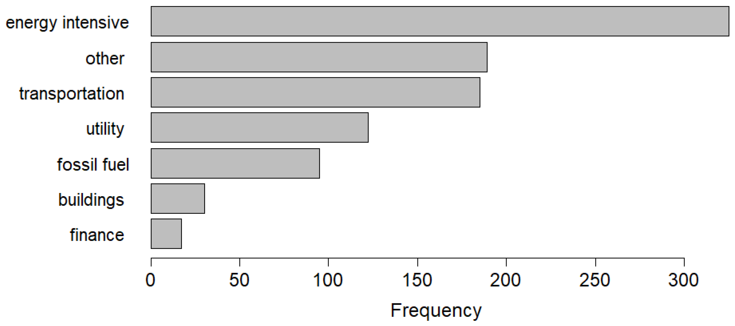
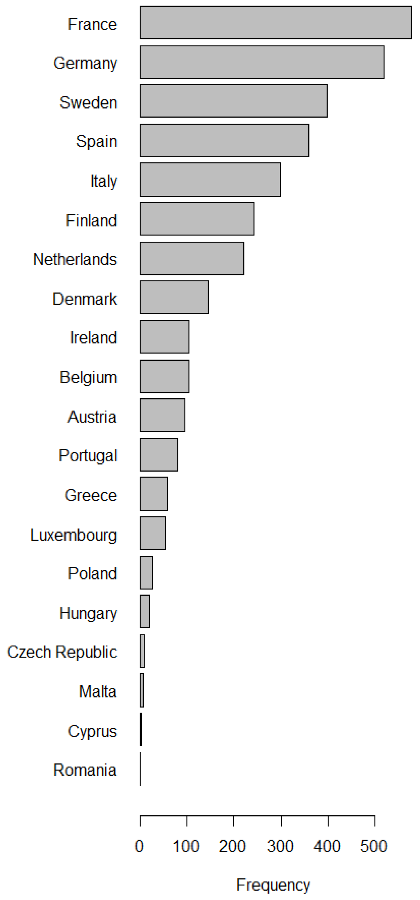
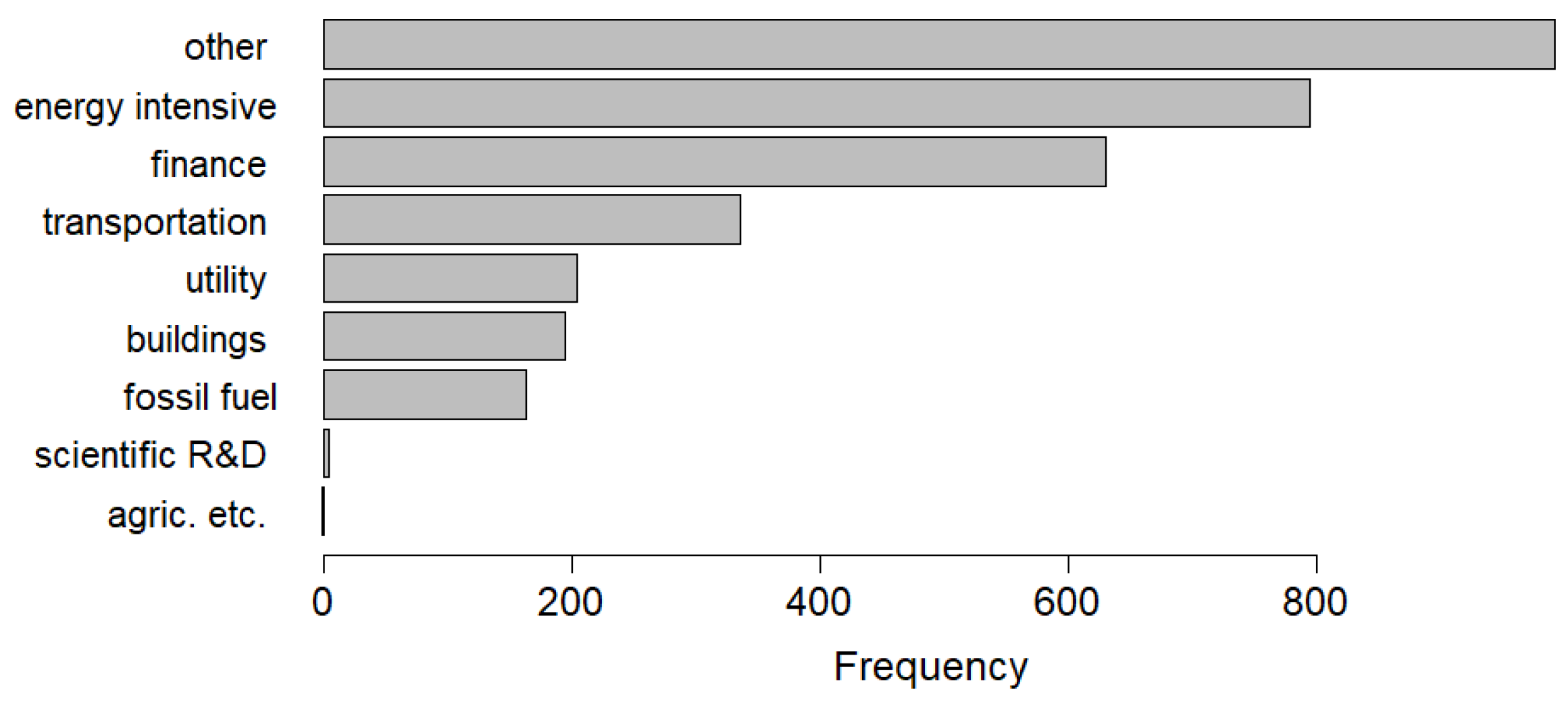
2.2. Sample and Data Exploration

Data about all variables of model (1), except $VA{T}_{i,t}$, have been downloaded from the Refinitiv (aka Thomson Reuters) database. Quantitative information about the VAT rate is instead provided by the OECD and the European Commission. Our original sample consisted of public and private firms whose headquarters are located in one of the 27 countries of the EU, and time-varying variables are observed at a yearly frequency for the period 2011–2020 ($T=10$). We did not consider firms located in other countries, because the ETS market of the EU, set up in 2005, is the oldest compared to all other ETS markets, such as those in New Zealand and South Korea. The longevity of the EU ETS market implies that we have enough time series observations for $PriceEU{A}_t$ to be able to detect a relationship between this variable and corporate revenues, in the time frame we consider.

This original sample underwent the following data cleaning process: negative values for revenues and total assets were set to “not available”; only unique firms, based on the International Securities Identification Number (ISIN), were kept in the sample; firm-year observations with missing values for any of the variables in Equation (1) were removed from the dataset; in order to obtain approximately Gaussian distributions for yearly percentage change of revenues, displayed in Figure 1a, we removed those firm-year observations above the 96th percentile of $\%\Delta Revenu{e}_{i,t}$. Our final sample is made of 693 companies, for a total of 3320 firm-year observations.

Figure 1b–d show the firm-average, over time, of $\%\Delta Revenu{e}_{i,t}$, $log{\left(Scope3\right)}_{i,t}$ and $priceEU{A}_t$, respectively. We notice that revenue growth and the EUAs price have mostly followed an upward trend over the past decade. Scope 3 emissions have, instead, fluctuated around a rather constant level. The main deviation from these tendencies was observed in 2020, which, due to the containment measures due to the COVID-19 pandemic, is characterized by the deepest fall in both revenues growth and Scope 3 emissions, and by a halt in the rise of the EUAs price.

The frequency of firm-year observations by country, size category, and NACE industry sector, are illustrated in Figure A1, Figure A2 and Figure A4, Appendix A, respectively. As expected, and with only a few exceptions, the majority of observations tend to be located in the largest national economies of the EU. As such, these countries are indeed abounding in companies.

When it comes to firms’ size, it is evident that almost the totality of observations in our sample refers to large companies. This massive concentration of one size category can be explained mostly by firms’ attitude to disclosing their Scope 3 emissions. Such information is usually shared by large companies, probably because their value chain tends to be more polluting, and they are thus under higher pressure to be transparent about their environmental impact. Moreover, they might have more resources to estimate their Scope 3 emissions—a process which is widely known to be challenging [51]. For the latter reason, data about Scope 3 emissions are generally characterized by several missing values, which pose a problem for quantitative analyses. In our case, the non-disclosing companies tend to be of smaller size, and are those who belong to the EU countries and NACE industry sectors are not shown in Figure A1 and Figure A4.

The latter figure is self-explanatory but also rather involved. Therefore, we complement and summarize it by displaying, in Figure A3, the frequency of firm-year observations in the economic sectors resulting from the Climate Policy Relevant Sectors (CPRS) classification of [37]. This is an aggregation of the NACE categories according to their relevance to climate mitigation policies (which we use only in this data exploration section, not for the estimation of model (1).

3. Empirical Results and Discussion

The discussion of the empirical results starts by investigating which value of $Scope{3}_{i,t}$ creates the coefficients’ disruption in Equation (1). Figure 2a displays the concentrated least-squares criterion $S\left(\gamma \right)$, for quantiles of Scope 3 emissions within their interdecile range. The criterion is minimized at the 71st quantile of $Scope{3}_{i,t}$, which is equivalent to $\widehat{\gamma }=619,628.4$ tonnes of emissions per year. Therefore, in our analysis we may deem “high” emitters along their value chain, those companies whose Scope 3 emissions are equal to or above 619,628.4 tonnes per year.

Figure 2b shows the Likelihood-Ratio test $LR\left(\gamma \right)$, for the same quantiles of Scope 3 emissions. Notice that $LR\left(\gamma \right)$ and $S\left(\gamma \right)$ follow the same pattern (which is implied by the expression for $LR\left(\gamma \right)$) but their scales (reported on the respective vertical axis) are different. In the same figure, we draw (with a dashed horizontal line) the 90% asymptotic critical value of $LR\left(\gamma \right)$, provided by [43], which can be used to test for the presence of a threshold. Quantiles of Scope 3 emissions corresponding to levels of $LR\left(\gamma \right)$ below the 90% asymptotic critical value are candidates for being the value of the threshold parameter. Hence, although $LR\left(\widehat{\gamma }\right)$ (i.e., $LR\left(\gamma \right)$ at the 71st quantile of $Scope{3}_{i,t}$) seems fairly distant from the other values of $LR\left(\gamma \right)$, our estimate of the threshold parameter $\widehat{\gamma }$, is subject to quite some uncertainty. Most of the other candidates are anyways gathered around the 70th quantile of $Scope{3}_{i,t}$, but there are also a few located near the 60th and 85th quantiles. Despite the uncertainty surrounding $\widehat{\gamma }$, which could already be improved if more observations for Scope 3 emissions were available, this result highlights that the coefficient disruption most likely occurs for values in the top half of the $Scope{3}_{i,t}$ distribution. This is in line with the expectation that climate reputational risk mainly affects companies whose value chain is already highly polluting.

Tabel

Table 1. Estimation results for regression (1). The sample size is made of $n=561$ companies and a total of 2504 firm-year observations. The coefficient estimates of the categorical regressors are omitted for the sake of simplicity. * p-value $<0.1$, ** p-value $<0.05$, *** p-value $<0.01$.

	Coefficient Estimate	Std. Error	t Statistic	p-Value
Intercept	5.82	12.39	0.47	0.64
$\%\Delta Revenu{e}_{i,t-1}$	0.07	0.02	3.64	2.8 × 10−9	***
$\%\Delta TotalAsset{s}_{i,t}$	0.21	0.01	16.07	2.2 × 10−16	***
$log\left(PriceEU{A}_{t}Scope{3}_{i,t}\right)$	−0.29	0.18	−1.62	0.11
$D_{i,t}$	13.43	5.85	2.29	0.02	**
$D_{i,t}log\left(PriceEU{A}_{t}Scope{3}_{i,t}\right)$	−0.63	0.34	−1.87	0.06	*
$VA{T}_{i,t}$	1.14	0.55	2.09	0.04	**
t	−0.64	0.11	−5.92	3.7 × 10−9	***
$\gamma$	619,628.4

reports the estimation results for model (1). Based on the sign and the significance of the coefficient estimates, we first conclude that $\%\Delta Revenu{e}_{i,t}$ is positively related to its previous value, $\%\Delta TotalAsset{s}_{i,t}$ and the VAT rate. (The latter result is in contrast with the above-discussed hypothesis of [30]. However, the empirical literature is unclear about the relationship between VAT and economic growth [52].) The negative impact of the linear time trend on revenue growth, which seems to be in contrast to what is observed in Figure 1b, can partly be explained by the presence of 2020 in our sample, and partly because the coefficient estimate at hand represents the effect of a “residual” time trend (which is left after projecting the dependent variable on the other regressors).

Moving on to the covariates of main interest, we notice that $\log \left(PriceEU{A}_{t}Scope{3}_{i,t}\right)$ is not significantly related to $\%\Delta Revenu{e}_{i,t}$, indicating that corporate revenues are not affected by the policy stringency, and hence climate reputational risk, for companies not having a high carbon footprint. On the contrary, the coefficient of $D_{i,t}\log \left(PriceEU{A}_{t}Scope{3}_{i,t}\right)$ is negative and significant at the 10% critical level. That is, for high Scope 3 emitters, a one percent increase in $PriceEU{A}_{t}Scope{3}_{i,t}$ (the climate policy stringency indicator) is expected to decrease $Revenu{e}_{i,t}$ by 0.0092 (=0.0029 + 0.0063) percentage points (ceteris paribus), due to climate reputational risk.

The parameter of $D_{i,t}$ is positive and significant at the 5% critical level, yielding an upward shift in the regression intercept. The coefficients disruption is illustrated in Figure 3. The solid line represents the marginal effect of $\log \left(PriceEU{A}_{t}Scope{3}_{i,t}\right)$ on $\%\Delta Revenu{e}_{i,t}$, ceteris paribus. We clearly see the intercept change, as well as a more pronounced downward slope, as Scope 3 emissions exceed the estimated threshold parameter. (Notice that, for the purpose of illustrating the coefficients disruption at $Scope{3}_{i,t}=\widehat{\gamma }$, Figure 3 reports $\%\Delta Revenu{e}_{i,t}$ on the vertical axis and the quantiles of $Scope{3}_{i,t}$ on the horizontal axis. However, the solid line represents the relationship not between these two variables, but between $\%\Delta Revenu{e}_{i,t}$ and $\log \left(PriceEU{A}_{t}Scope{3}_{i,t}\right)$, which explains why it is called “marginal effect of $\log \left(PriceEU{A}_{t}Scope{3}_{i,t}\right)$ on $\%\Delta Revenu{e}_{i,t}$”.)

In line with our expectations outlined in Section 2, the threshold regression model allowed us to identify a difference in climate reputational risk exposure between high and non-high Scope 3 emitters. Namely, companies that are not highly polluting along their value chain are not exposed to climate reputational risk. Conversely, high Scope 3 emitters are subject to revenue losses, because of the same risk. Through the estimation of the model, we found that we can target as “high” emitters those companies who produce at least 619,628.4 tonnes of Scope 3 emissions per year. However, this estimate is indicative as it is subject to some uncertainty, and should therefore be taken with caution. That is, firms with levels of Scope 3 emissions not far below this value are likely also to be subject to climate reputational risk.

The difference between the sample sizes reported in Table 1 and in Section 2.2 is due to the discarding of some observations, for the regression estimation, when lagging the dependent variable.

We conclude this section by analyzing which economic sectors are at higher climate reputational risk. Figure 4 and Figure 5 display the frequency of firm-year observations with $Scope{3}_{i,t}\ge \widehat{\gamma }$, by NACE and CPRS industry sectors, respectively. Compared to Figure A3 and Figure A4, we clearly notice that the most polluting sectors (in terms of Scope 3 emissions) have climbed the ranks. The manufacturing, energy intensive, transportation, utility, and fossil fuel sectors now occupy the highest positions, while leaving the last place for the finance business, and no more room for the scientific R&D and agricultural sectors.

4. Conclusions

With climate policies becoming increasingly stringent to ensure an emission trajectory compliant with the Paris Agreement goals, it is essential to understand the economic and financial impact of climate transition risk on companies’ economic and financial performances. The financial impact of transition risk, in particular, has so far been the main object of academic studies. The empirical models used, in fact, are backwards-looking and consider only emissions produced directly (Scope 1) and via energy consumption (Scope 2), hence neglecting the emissions along the value chain (Scope 3) that determine the product carbon footprint, which are certainly a significant source of market and reputational risk.

Understanding transition risk in the context of climate policy uncertainty requires new approaches that are forward-looking, consider all types of emissions and risk sources, and relate risk to the companies’ economics. Climate scenario analysis (CSA), used largely by financial and banking authorities to monitor the systemic exposure to transition risk and progressively being also adopted by financial institutions, is now becoming the new paradigm for measuring climate risk impacts at the company level.

While measuring the economic impacts of transition risk related to Scope 1 and Scope 2 emissions is relatively straightforward, being the impact related to carbon and energy prices increase, respectively, measuring the impact is more complex in the case of Scope 3. This paper adopts an empirical approach suitable to measure the impact of Scope 3 emissions on corporate revenues, accounting for non-linear impacts due to threshold effects and climate policy stringency.

Based on our empirical results, we conclude that high Scope 3 emitters are exposed to climate reputational risk, resulting in significantly increasing revenue losses as climate policies become more stringent. This implies that a climate policy stringency not only tends to reduce GHG emissions, but also affects the market through reputational risk. Moreover, we find, as expected, that the firms most exposed to climate reputational risk belong to those industry sectors with the most polluting value chain, such as the manufacturing one.

From an operational point of view, our findings reveal that firms’ reputations might be at stake not only because of their Scope 1 and 2 emissions, but also because of the emissions produced along their value chain. Companies can use our results to understand whether they are at (potential) risk of reputational damage because of their carbon footprint, and in that case, to indicatively quantify the impact of such risk exposure on their business performance. Additionally, by adopting a methodology that links corporate Scope 3 emissions to a climate policy stringency, our work calls on firms to be forward-looking by defining a decarbonization plan for their value chain. This would allow them to mitigate climate reputational risk, and thus avoid more severe economic damage in the future. However, we also caution companies to take the uncertainty surrounding our results into account when defining action plans based on the latter.

Our paper is uniquely located at the intersection of the literature on climate scenario analysis (CSA) and climate reputational risk. As such, it has the limitation of having results that are not easily comparable to related research. Similarly to us, [30] modeled the impact of climate reputational risk on corporate revenues through a pre-defined value added tax (VAT) rate increase for companies with high Scope 3 emissions. We instead provide a methodology to estimate the same impact from the data, and to condition it with a typical climate policy instrument (instead of the VAT). Additionally, the statistical significance of our results confirms the finding of [31] that climate reputational risk is associated with Scope 3 emissions.

References

1. Pörtner, H.O.; Roberts, D.C.; Adams, H.; Adler, C.; Aldunce, P.; Ali, E.; Begum, R.A.; Betts, R.; Kerr, R.B.; Biesbroek, R.; et al. Climate Change 2022: Impacts, Adaptation and Vulnerability. In IPCC Sixth Assessment Report; United Nations: New York, NY, USA, 2022; pp. 37–118. [Google Scholar]
2. Newbold, T.; Oppenheimer, P.; Etard, A.; Williams, J.J. Tropical and Mediterranean Biodiversity is Disproportionately Sensitive to Land-use and Climate Change. Nat. Ecol. Evol. 2020, 4, 1630–1638. [Google Scholar] [CrossRef] [PubMed]
3. Sillmann, J.; Aunan, K.; Emberson, L.; Büker, P.; Van Oort, B.; O’Neill, C.; Otero, N.; Pandey, D.; Brisebois, A. Combined Impacts of Climate and Air Pollution on Human Health and Agricultural Productivity. Environ. Res. Lett. 2021, 16, 093004. [Google Scholar] [CrossRef]
4. Kaczan, D.J.; Orgill-Meyer, J. The Impact of Climate Change on Migration: A Synthesis of Recent Empirical Insights. Clim. Chang. 2020, 158, 281–300. [Google Scholar] [CrossRef]
5. Trenberth, K.E.; Fasullo, J.T.; Shepherd, T.G. Attribution of Climate Extreme Events. Nat. Clim. Chang. 2015, 5, 725–730. [Google Scholar] [CrossRef]
6. Overpeck, J.T.; Conde, C. A Call to Climate Action. Science 2019, 364, 807. [Google Scholar] [CrossRef] [PubMed] [Green Version]
7. OECD. Investing in Climate, Investing in Growth; OECD: Paris, France, 2017; p. 312. [Google Scholar]
8. Challinor, A.J.; Watson, J.; Lobell, D.B.; Howden, S.; Smith, D.; Chhetri, N. A Meta-analysis of Crop Yield under Climate Change and Adaptation. Nat. Clim. Chang. 2014, 4, 287–291. [Google Scholar] [CrossRef] [Green Version]
9. Chen, C.C.; McCarl, B.A.; Schimmelpfennig, D.E. Yield Variability as Influenced by Climate: A Statistical Investigation. Clim. Chang. 2004, 66, 239–261. [Google Scholar] [CrossRef] [Green Version]
10. Frank, S.; Böttcher, H.; Gusti, M.; Havlík, P.; Klaassen, G.; Kindermann, G.; Obersteiner, M. Dynamics of the Land Use, Land Use Change, and Forestry Sink in the European Union: The Impacts of Energy and Climate Targets for 2030. Clim. Chang. 2016, 138, 253–266. [Google Scholar] [CrossRef] [Green Version]
11. Hasegawa, T.; Fujimori, S.; Havlík, P.; Valin, H.; Bodirsky, B.L.; Doelman, J.C.; Fellmann, T.; Kyle, P.; Koopman, J.F.; Lotze-Campen, H.; et al. Risk of Increased Food Insecurity under Stringent Global Climate Change Mitigation Policy. Nat. Clim. Chang. 2018, 8, 699–703. [Google Scholar] [CrossRef] [Green Version]
12. Hatfield, J.L.; Boote, K.J.; Kimball, B.A.; Ziska, L.; Izaurralde, R.C.; Ort, D.; Thomson, A.M.; Wolfe, D. Climate Impacts on Agriculture: Implications for Crop Production. Agron. J. 2011, 103, 351–370. [Google Scholar] [CrossRef] [Green Version]
13. Huntingford, C.; Zelazowski, P.; Galbraith, D.; Mercado, L.M.; Sitch, S.; Fisher, R.; Lomas, M.; Walker, A.P.; Jones, C.D.; Booth, B.B.; et al. Simulated Resilience of Tropical Rainforests to CO2-Induced Climate Change. Nat. Geosci. 2013, 6, 268–273. [Google Scholar] [CrossRef]
14. Leclère, D.; Havlík, P.; Fuss, S.; Schmid, E.; Mosnier, A.; Walsh, B.; Valin, H.; Herrero, M.; Khabarov, N.; Obersteiner, M. Climate Change Induced Transformations of Agricultural Systems: Insights from a Global Model. Environ. Res. Lett. 2014, 9, 124018. [Google Scholar] [CrossRef]
15. Nelson, G.C.; Valin, H.; Sands, R.D.; Havlík, P.; Ahammad, H.; Deryng, D.; Elliott, J.; Fujimori, S.; Hasegawa, T.; Heyhoe, E.; et al. Climate Change Effects on Agriculture: Economic Responses to Biophysical Shocks. Proc. Natl. Acad. Sci. USA 2014, 111, 3274–3279. [Google Scholar] [CrossRef] [Green Version]
16. Alfieri, L.; Feyen, L.; Dottori, F.; Bianchi, A. Ensemble Flood Risk Assessment in Europe under High end Climate Scenarios. Glob. Environ. Chang. 2015, 35, 199–212. [Google Scholar] [CrossRef]
17. Camia, A.; Libertá, G.; San-Miguel-Ayanz, J. Modeling the Impacts of Climate Change on Forest Fire Danger in Europe. Jt. Res. Cent. (JRC) Tech. Rep. 2017, 1, 22. [Google Scholar]
18. Hinkel, J.; Jaeger, C.; Nicholls, R.J.; Lowe, J.; Renn, O.; Peijun, S. Sea-level Rise Scenarios and Coastal Risk Management. Nat. Clim. Chang. 2015, 5, 188–190. [Google Scholar] [CrossRef]
19. Semieniuk, G.; Campiglio, E.; Mercure, J.F.; Volz, U.; Edwards, N.R. Low-carbon Transition Risks for Finance. Wiley Interdiscip. Rev. Clim. Chang. 2021, 12, e678. [Google Scholar] [CrossRef]
20. Bertram, C.; Hilaire, J.; Kriegler, E.; Beck, T.; Bresch, D.; Clarke, L.; Cui, R.; Edmonds, J.; Min, J.; Piontek, F.; et al. NGFS Climate Scenarios Database: Technical Documentation; NGFS: Paris, France, 2020. [Google Scholar]
21. Zhang, S.Y. Are Investors Sensitive to Climate-related Transition and Physical Risks? Evidence from Global Stock Markets. Res. Int. Bus. Financ. 2022, 62, 101710. [Google Scholar] [CrossRef]
22. Monasterolo, I.; De Angelis, L. Blind to Carbon Risk? An Analysis of Stock Market Reaction to the Paris Agreement. Ecol. Econ. 2020, 170, 106571. [Google Scholar] [CrossRef]
23. Bolton, P.; Kacperczyk, M. Do Investors Care about Carbon Risk? J. Financ. Econ. 2021, 142, 517–549. [Google Scholar] [CrossRef]
24. Ilhan, E.; Sautner, Z.; Vilkov, G. Carbon Tail Risk. Rev. Financ. Stud. 2021, 34, 1540–1571. [Google Scholar] [CrossRef]
25. Alessi, L.; Ossola, E.; Panzica, R. What Greenium Matters in the Stock Market? The Role of Greenhouse Gas Emissions and Environmental Disclosures. J. Financ. Stab. 2021, 54, 100869. [Google Scholar] [CrossRef]
26. Basse Mama, H.; Mandaroux, R. Do Investors Care About Carbon Emissions under the European Environmental Policy? Bus. Strategy Environ. 2022, 31, 268–283. [Google Scholar] [CrossRef]
27. TCFD. Recommendations of the Task Force on Climate-Related Financial Disclosures; TCFD: New York, NY, USA, 2017. [Google Scholar]
28. FSB-NGFS. Climate Scenario Analysis by Jurisdictions: Initial Findings and Lessons; Financial Stability Board: Basel, Switzerland, 2022. [Google Scholar]
29. Dai, R.; Duan, R.; Liang, H.; Ng, L. Enabling Full Supply Chain Corporate Responsibility: Scope 3 Emissions Targets for Ambitious Climate Change Mitigation; Finance Working Paper No. 723/2021; European Corporate Governance Institute: Brussels, Belgium, 2021. [Google Scholar]
30. Alogoskoufis, S.; Dunz, N.; Emambakhsh, T.; Hennig, T.; Kaijser, M.; Kouratzoglou, C.; Muñoz, M.A.; Parisi, L.; Salleo, C. ECB Economy-Wide Climate Stress Test: Methodology and Results; Occasional Paper Series; European Central Bank: Frankfurt, Germany, 2021. [Google Scholar]
31. Dai, R.; Duan, R.; Liang, H.; Ng, L. Outsourcing Climate Change; Finance Working Paper No. 723/2021; European Corporate Governance Institute: Brussels, Belgium, 2021. [Google Scholar]
32. Scott, M.; Van Huizen, J.; Jung, C. The Bank’s Response to Climate Change; Bank of England Quarterly Bulletin; Bank of England: London, UK, 2017; p. Q2. [Google Scholar]
33. Vermeulen, R.; Schets, E.; Lohuis, M.; Kolbl, B.; Jansen, D.J.; Heeringa, W. An Energy Transition Risk Stress Test for the Financial System of the Netherlands; Research Department, Netherlands Central Bank: Amsterdam, The Netherlands, 2018. [Google Scholar]
34. Gros, D.; Lane, P.R.; Langfield, S.; Matikainen, S.; Pagano, M.; Schoenmaker, D.; Suarez, J. Too Late, Too Sudden: Transition to a Low-Carbon Economy and Systemic Risk; Number 6, Reports of the Advisory Scientific Committee; ESRB: New York, NY, USA, 2016. [Google Scholar]
35. Allen, T.; Dees, S.; Caicedo Graciano, C.M.; Chouard, V.; Clerc, L.; de Gaye, A.; Devulder, A.; Diot, S.; Lisack, N.; Pegoraro, F.; et al. Climate-Related Scenarios for Financial Stability Assessment: An Application to France; Banque de France Working Paper; Banque de France: Paris, France, 2020. [Google Scholar]
36. Vermeulen, R.; Schets, E.; Lohuis, M.; Kölbl, B.; Jansen, D.J.; Heeringa, W. The Heat is on: A Framework for Measuring Financial Stress under Disruptive Energy Transition Scenarios. Ecol. Econ. 2021, 190, 107205. [Google Scholar] [CrossRef]
37. Battiston, S.; Mandel, A.; Monasterolo, I.; Schütze, F.; Visentin, G. A Climate Stress-test of the Sinancial System. Nat. Clim. Chang. 2017, 7, 283–288. [Google Scholar] [CrossRef]
38. Chenet, H. Climate Change and Financial Risk; Springer: Berlin/Heidelberg, Germany, 2021. [Google Scholar]
39. Hogan, J.; Lodhia, S. Sustainability Reporting and Reputation Risk Management: An Australian Case Study. Int. J. Account. Inf. Manag. 2011, 19, 267–287. [Google Scholar] [CrossRef]
40. Blanco, C.; Caro, F.; Corbett, C.J. The State of Supply Chain Carbon Footprinting: Analysis of CDP Disclosures by US Firms. J. Clean. Prod. 2016, 135, 1189–1197. [Google Scholar] [CrossRef] [Green Version]
41. Guastella, G.; Mazzarano, M.; Pareglio, S.; Xepapadeas, A. Climate Reputation Risk and Abnormal Returns in the Stock Markets: A Focus on Large Emitters. Int. Rev. Financ. Anal. 2022, 84, 102365. [Google Scholar] [CrossRef]
42. Diaz-Rainey, I.; Gehricke, S.A.; Roberts, H.; Zhang, R. Trump vs. Paris: The Impact of Climate Policy on US Listed Oil and Gas Firm Returns and Volatility. Int. Rev. Financ. Anal. 2021, 76, 101746. [Google Scholar] [CrossRef]
43. Hansen, B.E. Sample Splitting and Threshold Estimation. Econometrica 2000, 68, 575–603. [Google Scholar] [CrossRef] [Green Version]
44. Wooldridge, J.M. Selection Corrections for Panel Data Models Under Conditional Mean Independence Assumptions. J. Econom. 1995, 68, 115–132. [Google Scholar] [CrossRef]
45. OECD. OECD SME and Entrepreneurship Outlook: 2005; OECD: Paris, France, 2005; p. 17. [Google Scholar]
46. Eurostat. NACE Rev. 2 Statistical Classification of Economic Activities in the European Community; Methodologies and Working Papers; Eurostat: Luxembourg, 2008. [Google Scholar]
47. Downie, J.; Stubbs, W. Corporate Carbon Strategies and Greenhouse Gas Emission Assessments: The Implications of Scope 3 Emission Factor Selection. Bus. Strategy Environ. 2012, 21, 412–422. [Google Scholar] [CrossRef]
48. European Commission. EU ETS Handbook; European Commission: Bangkok, Thailand, 2015. [Google Scholar]
49. Hansen, B.E. Econometrics; Princeton University Press: Princeton, NJ, USA, 2022. [Google Scholar]
50. Chan, K.S. Consistency and Limiting Distribution of the Least Squares Estimator of a Threshold Autoregressive Model. Ann. Stat. 1993, 21, 520–533. [Google Scholar] [CrossRef]
51. Schmidt, M.; Nill, M.; Scholz, J. Determining the Scope 3 Emissions of Companies. Chem. Eng. Technol. 2022, 45, 1218–1230. [Google Scholar] [CrossRef]
52. Gale, G.W.; Gelfond, H.; Krupkin, A. Entrepreneurship and Small Business Under a Value-Added Tax; Economic Studies at Brookings; Brookings: Washington, DC, USA, 2016. [Google Scholar]
Figure 1. Descriptive plots of the variables of main interest. (a) Histogram of % Δ R e v e n u e i , t ; (b) Firm-average of % Δ R e v e n u e i , t ; (c) Firm-average of log ( S c o p e 3 ) i , t ; (d) Time series of p r i c e E U A t .
Sustainability 15 05886 g001
Figure 2. Plots of the concentrated least-squares criterion and the Likelihood-Ratio test. (a) Concentrated least-squares criterion S ( γ ) (solid line) for quantiles of S c o p e 3 i , t . The dashed line represents the 71st quantile of Scope 3 emissions, which corresponds to γ ^ = 619 , 628.4 tonnes per year; (b) Likelihood-Ratio test L R ( γ ) , for a threshold parameter (solid line). The horizontal axis reports the quantiles of S c o p e 3 i , t . The dashed line represents the 90% asymptotic critical value of L R ( γ ) .
Sustainability 15 05886 g002
Figure 3. Marginal effect of log ( P r i c e E U A t S c o p e 3 i , t ) , ceteris paribus, when Scope 3 emissions fall below (left-hand solid line) and above (right-hand solid line) their 71st quantile. The horizontal axis reports the quantiles of S c o p e 3 i , t . The dashed line represents the 71st quantile of Scope 3 emissions, which corresponds to γ ^ = 619,628.4 tonnes per year.
Sustainability 15 05886 g003
Figure 4. Frequency of firm-year observations with S c o p e 3 i , t γ ^ , by NACE industry sector.
Sustainability 15 05886 g004
Figure 5. Frequency of firm-year observations with S c o p e 3 i , t γ ^ , by CPRS industry sector.
Sustainability 15 05886 g005