Article

Affecting of Nature and Human Activities on the Trend of Vegetation Health Indices in Dak Nong Province, Vietnam

1
Institute of Environmental Science, Engineering and Management, Industrial University of Ho Chi Minh City, Ho Chi Minh City 700000, Vietnam
2
Department of Natural Resources and Environment of Dak Nong Province, Gia Nghia 641190, Vietnam
*
Author to whom correspondence should be addressed.
Sustainability 2023, 15(7), 5695; https://doi.org/10.3390/su15075695
Submission received: 5 February 2023 / Revised: 8 March 2023 / Accepted: 22 March 2023 / Published: 24 March 2023

Abstract

:
This study aims to evaluate the effects of natural and human conditions on vegetation covers using VCI and TCI indices (the satellite-based Vegetation Health Indices (VHIs)) in Dak Nong province. Factors affecting the VHIs included in the analysis involve land use, soil, population, topography, distance to roads and surface water. The data analysis period is the dry season from 2000 to 2020. The trend of the VHIs’ change in this study is analyzed using Sen’s method with monitoring data from Modis. The effects of factors affecting the VHIs are based on logistic regression and discriminant analysis. The analysis results show that the VHIs are clear and show both increasing and decreasing trends. Based on logistic regression analysis, the influence of land use types on the trend of the VHIs in the direction of increasing from negative to positive will be from PdF, UnL, AnC, SpF, PtF, PeA and then to PdR. Corresponding to the soil will be from ACa, FRp, FRx, FRr, ACh, LVx, FLg and then to LVg. Based on the discriminant analysis method, it was found that there are only four primary factors affecting the trend of the VHIs in order of decreasing level of closure: population density, land use, soil and population growth rate and to the road. These results show that in places where labour resources are available, plants are interested in investment due to high profits, nutrient-rich soil and convenience for plant care; the VHIs tend to increase and vice versa. Compared with VCI, the trend of TCI tends to be sloping negative and more pessimistic. Through the coefficients of the logistic regression equation and the difference function, the TCI is more sensitive than the VCI when the independent variables change, especially for changes in population density and land use. Thus, TCI can be considered the preferred option for assessing vegetation health trends in the context of climate change.

1. Introduction

Vegetation is an important component of terrestrial ecosystems [1]. The vegetation status is related to the carbon storage capacity on the continent, crop yields, surface energy exchange, water balance and microclimate conditions [2,3,4,5]. Today, due to the impacts of climate change, population growth and accompanying needs, vegetation has changed rapidly [1,6,7,8]. Therefore, analyzing the trend of vegetation is necessary to contribute to the development and protection of the ecosystem [1]. Numerous scientists regard the vegetation index as an important measure for mapping agricultural fields, monitoring rainfall, evaluating weather impacts, calculating biomass, crop output, pasture production and drought conditions and determining the vitality of the vegetation [9].
With the advancement of satellite photography, agricultural monitoring systems have employed indices derived from the spectral reflectance of vegetation to offer timely and precise information regarding seasonal vegetative growth [10]. Assessing changes or trends in vegetation cover is often based on remote sensing indicators. In 1969, Kriegler et al. [11] proposed a simple band transformation by the near-infrared radiation (NIR), subtracting the red radiation (RED) and dividing by their sum to produce an image called the Normalized Difference Vegetation Index (NDVI). This index is sensitive to phenology and anthropogenic effects; therefore, it is widely used in monitoring the growth and variability of vegetation [11,12,13,14,15,16]. NDVI has a good relationship with several characteristics of vegetation, such as vegetation cover, leaf area index [17], photosynthetic radiation absorption capacity, biomass [13,18], leaf chlorophyll concentration [19], plant stress [20] and crop yield [21]. NDVI is also widely used to explore the relationship between vegetation conditions and climate change [1,22].
The Vegetation Condition Index (VCI) is a normalized form of the NDVI data series over time. This index is widely used in assessing vegetation health and cover changes and in assessing vegetation stresses, including drought [23,24].
Land use change has changed the properties of the cover and made the surface temperature (LST) change markedly [25,26]. LST changes lead to altering air temperature and habitat [27]. In addition to using LST to monitor environmental temperature, it is also used to assess changes in cover due to temperature conditions. Because the statistical characteristics of LST are different between months, the Temperature Condition Index (TCI) is often used to replace LST. TCI allows analyzing the effect of temperature on vegetation health. Low values of TCI indicate plant stress due to high temperatures and are often associated with low soil moisture. A high TCI value indicates healthy vegetation [28].
TCI is often combined with VCI to assess vegetation cover variability, health and plant stress related to temperature and humidity conditions [25,29,30,31,32,33]. The vegetation status can be detected based on VCI and TCI [34]. Some studies [35] suggested that VCI is a more accurate indicator to assess the vegetation cover condition, whereas others suggested TCI [36].
The change in land use makes VCI and TCI have a clear trend, and many studies are in this direction [5,7,8,37,38]. Vegetation ensures ecosystem sustainability by preventing soil erosion, reducing nutrient loss and maintaining hydrological cycles [25]. Characteristic change of the vegetation cover is one of the crucial factors in environmental vulnerability [39]. In the stable land use types, the trend of VCI and TCI is the question posed and solved in this study. The main contents are carried out to identify the causes related to the trend of land use types and the sensitivity of vegetation indicators, contributing to the monitoring and sustainable development of the cover.

2. Data and Methods

2.1. Data

This study used data including NDVI and LST and data related to population, soil and land use in the study area. NDVI and LST are used to calculate the VHIs. The 2000–2020 time series of NDVI and LST derived from the MODIS are used in this study (source: https://earthexplorer.usgs.gov/) (accessed on 25 October 2022). However, the clouds affected the quality of the obtained images; therefore, this study used the images from January to April because there is low cloud in dry season.
The NDVI data are derived from the Mod13A1 VI package, which is a product of MODIS. This data has a spatial resolution of 463 m × 463 m and a temporal resolution of 16 days. Due to orbital overlap, multiple observations can exist in one day, and up to 64 observations can be collected in 16 days. Furthermore, due to the influence of clouds and other atmospheric conditions, the acceptable number of pixels is usually concentrated between 1 and 5. To eliminate these effects, the technique of a maximum value composite is used in building this package. Finally, LST data are obtained from the Mod11A2 package. This data has a spatial resolution of 926.6 m × 926.6 m and a temporal resolution of 8 days.
Population data were collected during the 1999, 2009 and 2019 censuses. These data were collected for each commune in Dak Nong province. The administrative boundaries of the study area are as shown in Figure 1, with 8 districts and 71 communes.
Soil and land use data were obtained from the Department of Agriculture and Rural Development of Dak Nong province at the beginning and end of the study period. In the study area, there are seven types of land use and eight main types of soil, as shown in Table 1 and Table 2.
In Table 1, protection forests are used mainly to protect water sources and land, prevent erosion and restrict natural calamities. Special-use forests are used mainly for the conservation of nature, specimens of the national forest ecosystems and forest biological gene sources. Production forests are used mainly for producing and trading timber and non-timber forest products in combination with protection. Unused land includes the land types for which land use purposes have yet to be determined. This area’s perennial plants are mainly coffee, rubber, cashew, pepper and Macca. The annual plants are mainly paddy rice, upland rice, maize, cassava, beans and vegetables. Due to the critical role of paddy rice, it is separated.

2.2. Methods

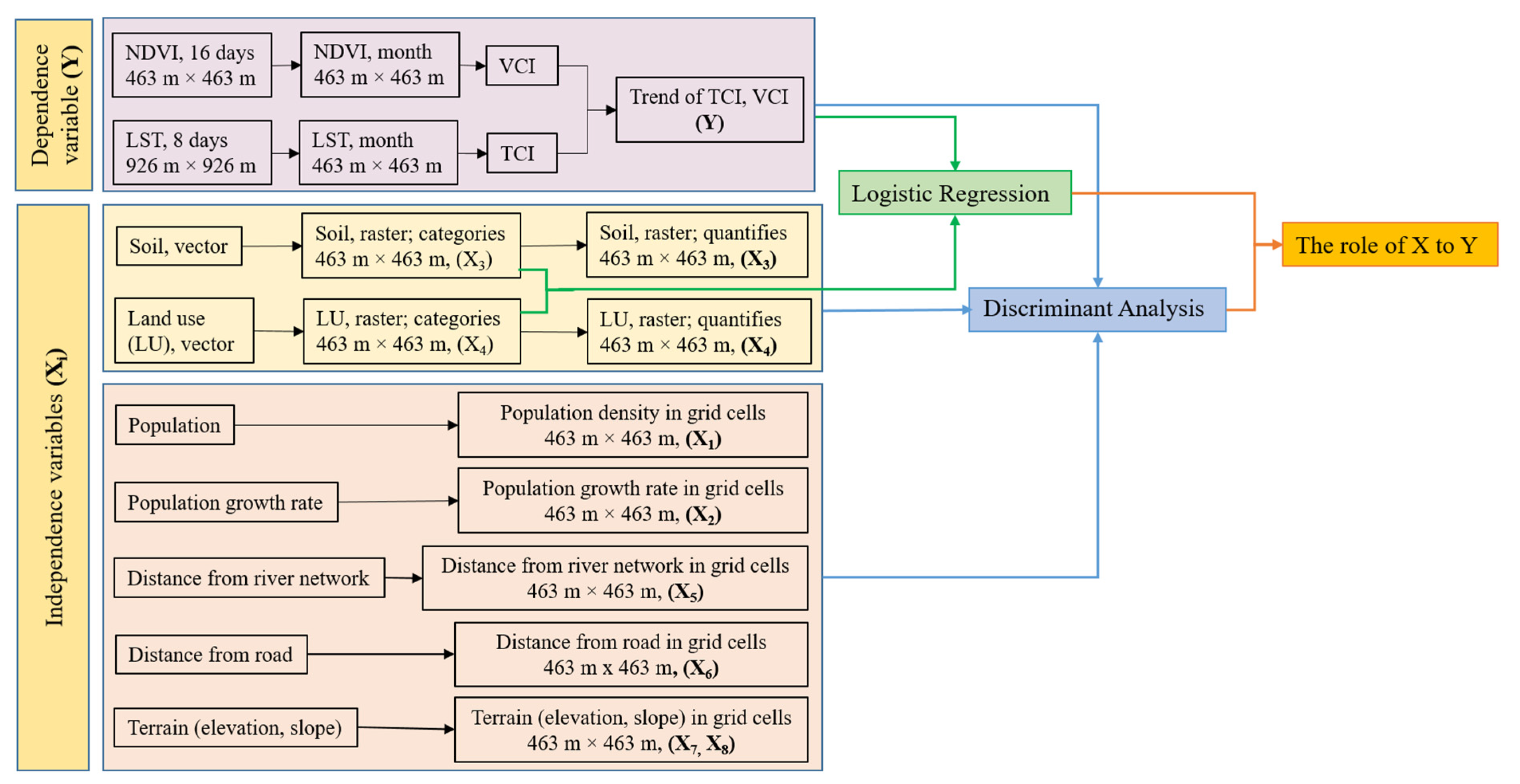
The objective of this study is to analyse the trends of the VHIs and assess the influence of population distribution, soil and land use on these indices’ trends. The general workflow performed in this study is shown in the diagram below (Figure 2).
With these steps, the implementation methods for these steps are as follows:
  • Re-sample and determine NDVI and LST monthly;
In this study, the indices derived from the satellite need to convert to the same spatial and temporal resolution. The time scale of VHI chosen in this study was monthly. Then, the maximum value composite method was applied to obtain monthly NDVI data to reduce the atmospheric impact from the NDVI input data with a 16-days temporal resolution. Meanwhile, the average monthly LST was calculated from Mod11A2 packages with 8-day temporal resolution. Therefore, to have the same spatial resolution, the average monthly LST was re-sampled to the same resolution as NDVI. The method used in re-sampling is bilinear. After NDVI and LST have been converted to the same spatial and temporal resolution, VCI and TCI will be calculated, and their relationship with the population distribution will be determined.
  • VCI calculation;
The VCI is the normalized value of NDVI over time [40]; the VCI formula is shown as below:
V C I = 100 N D V I i N D V I m i n N D V I m a x N D V I m i n
where NDVIi is the NDVI value of the pixel in a particular year at the time i; NDVImax and NDVImin are the highest value of NDVI and the lowest value of NDVI for an observation period included in the analysis, respectively. The numerator is the difference between the actual and the lowest value of the NDVI and represents the state of plant growth and meteorological conditions. The maximum and minimum values of the denominator reflect the best and worst growth conditions, and the difference between them partly reflects the conditions of the local vegetation. Therefore, the VCI contains both historical and real-time information on NDVI. VCI ranges from 0 to 100, where smaller VCI values indicate underdeveloped plants and a higher degree of drought. VCI is often used in conjunction with TCI in assessing drought severity and crop health. In this study, VCI is calculated for each month in the dry season, from 2000 to 2020.
  • TCI calculation;
TCI was developed by Kogan [40]; it is normalized from LST over time and is shown in the formula below:
T C I = 100 L S T m a x L S T L S T m a x L S T m i n
where LSTi is the LST value at a pixel at the time i; LSTmax and LSTmin are the maximum and minimum LST values for an observation period included in the analysis at the analyzed pixel, respectively. This index is used to assess variations in surface temperature and coating variation. According to this formula, the TCI will have a value between 0 and 100 and have the highest value when LST is the lowest. This study calculated TCI for each month in the dry season, from 2000 to 2020.
  • Trend of the VHIs;
The determination of the trend of the VHIs is carried out according to grid cells that have no change in land use in the period of 2000–2020. This study uses Sen’s method and the Mann–Kendall non-parametric test to determine the trend. Luong [41] presents details of the Mann–Kendall test method.
For the time series x1, x2, … xn, in the method determining Sen’s slope, the magnitude of the trend is determined as the median of the range of n(n − 1)/2 elements {(xjxk)/(j − k), where k = 1, 2, …, n − 1; j > k}. The VHIs’ data for this study are 4 months during the dry season in 21 years; therefore, the data for analysis is 84, and the most significant difference of jk is = (21 − 1) × 12 + 4 − 1 = 243 months. Where 12 is the number of months in a year, 4 is the fourth month of the end year, and 1 is the first month of the starting year.
  • Raster data of the independent variables;
To facilitate the analysis of data layers on population density, population growth rate, land use and soil are converted to raster. The data on population density and population growth rate are converted to raster-based on the assumption that they are evenly distributed over the communes. The Euclidean distance tool is used to create the distances to rivers and major roads. The raster data of all the independent variables have the same resolution as the data of the VHIs of 463 m × 463 m.
  • Logistic regression;
Logistic regression is used to build the relationship between the dependent variable, the trend of the VHIs and the independent variables in the categories of soil and land use. These variables are taken in the grid cells where the VHIs have a clear trend with a significance level (p = 0.01). In order to ensure the quality of the regression equation, the VHIs’ trend is only analyzed in a binary form showing its upward or downward trend.
The logistic regression equation is stated as below:
l o g p 1 p = b 0 + b 1 x 1 + b 2 x 2 + + b n x n
where p and p − 1 are the probability for the VHIs to have an upward or downward trend, respectively. In this equation, X = (x1, x2, x3, …, xn) are independent variables, and the coefficients b0, b1, b2, b3, …, bn are estimated based on a regression equation.
  • Discriminant Analysis.
Discriminant analysis was used to determine the role of factors influencing the the VHIs’ trend. Influential variables include topography, distance to rivers, lakes and roads, population density and growth rate, and soil and land use. These variables are also taken in the grid cells where the VHIs have a significant trend at the significance level (p = 0.01).
The discriminant analysis also requires the dependent variables to be grouping variables. As with the logistic regression, the dependent variables (the VHIs’ trends) are divided into two groups: increasing and decreasing and only considered on the grid cells having a significance level (p = 0.01). Due to the requirement of discriminant analysis that the independent variables must be in quantities form, the data on land use and soil in categories form should be converted to this required form. The conversion is based on the probability of an uptrend of the VHIs across soil types and land use types.

3. Results and Discussion

This section may be divided by subheadings. It should provide a concise and precise description of the experimental results and their interpretation, as well as the experimental conclusions that can be drawn.

3.1. VHIs’ Trend

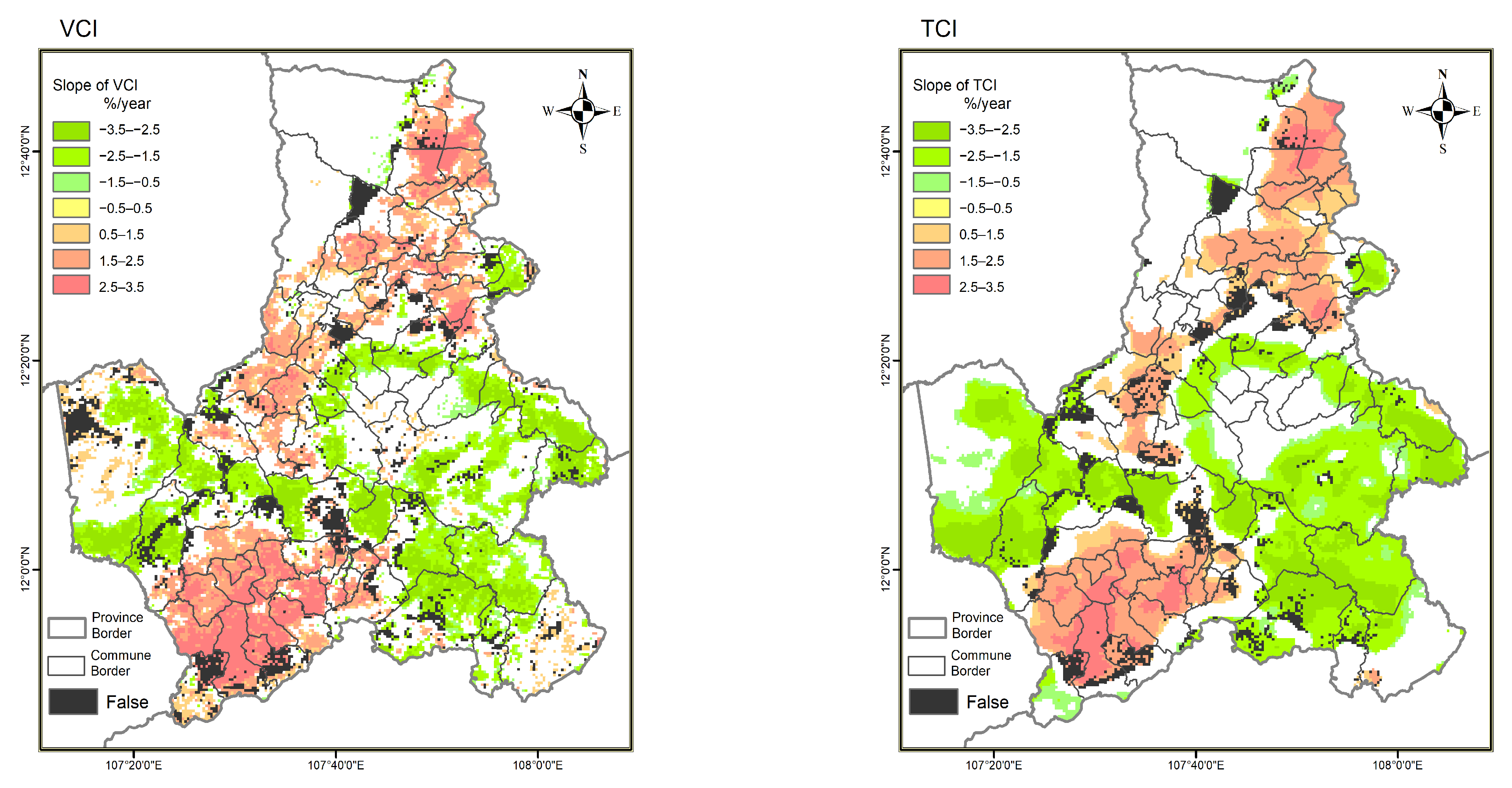
From the data of VCI and TCI with conversion to the 463 m × 463 m resolution and applied Sen’s method, the determined trend result is shown in Figure 3. The coloured cells in this figure have a significance level of 0.01; the rest tend to be indeterminate. The results show a relative relationship between the trends of VCI and TCI. According to these figures, the trend of the VHIs tends to be different in some regions; some places show an upward trend, some are unclear and some decrease.
Statistical results from these figures show that VCI’s trend does not have a significant difference in the three parts of increase, decrease and unclear trend, with values of 32%, 31% and 37%, respectively. Meanwhile, unlike VCI, these parts in TCI are relatively different, with values of 27%, 42% and 31%, respectively. Thus, TCI tends to decrease significantly; the decreasing area is higher than the increased area, by approximately 1.6 times. Total areas with evident trends for VCI and TCI are 63% and 69%, respectively, or TCI is more sensitive to vegetation health. Compared with VCI, TCI’s trend is more negative and could be related to the increase in temperature due to climate change. This result was calculated for the dry season months and is consistent with the research of Kukunuri et al. [42] that compared with VCI, TCI is more sensitive in arid to extremely arid conditions.
The marked increase and decrease of the VHIs are usually over 0.5%/year. The highest increase and decrease are of approximately 3.5%/year, and the overall is mainly within the range of 1.5–2.5%/year (Figure 3). Thus, from 2000 to 2020, many places experienced an increase or decrease in these indicators from 30% to 50%.
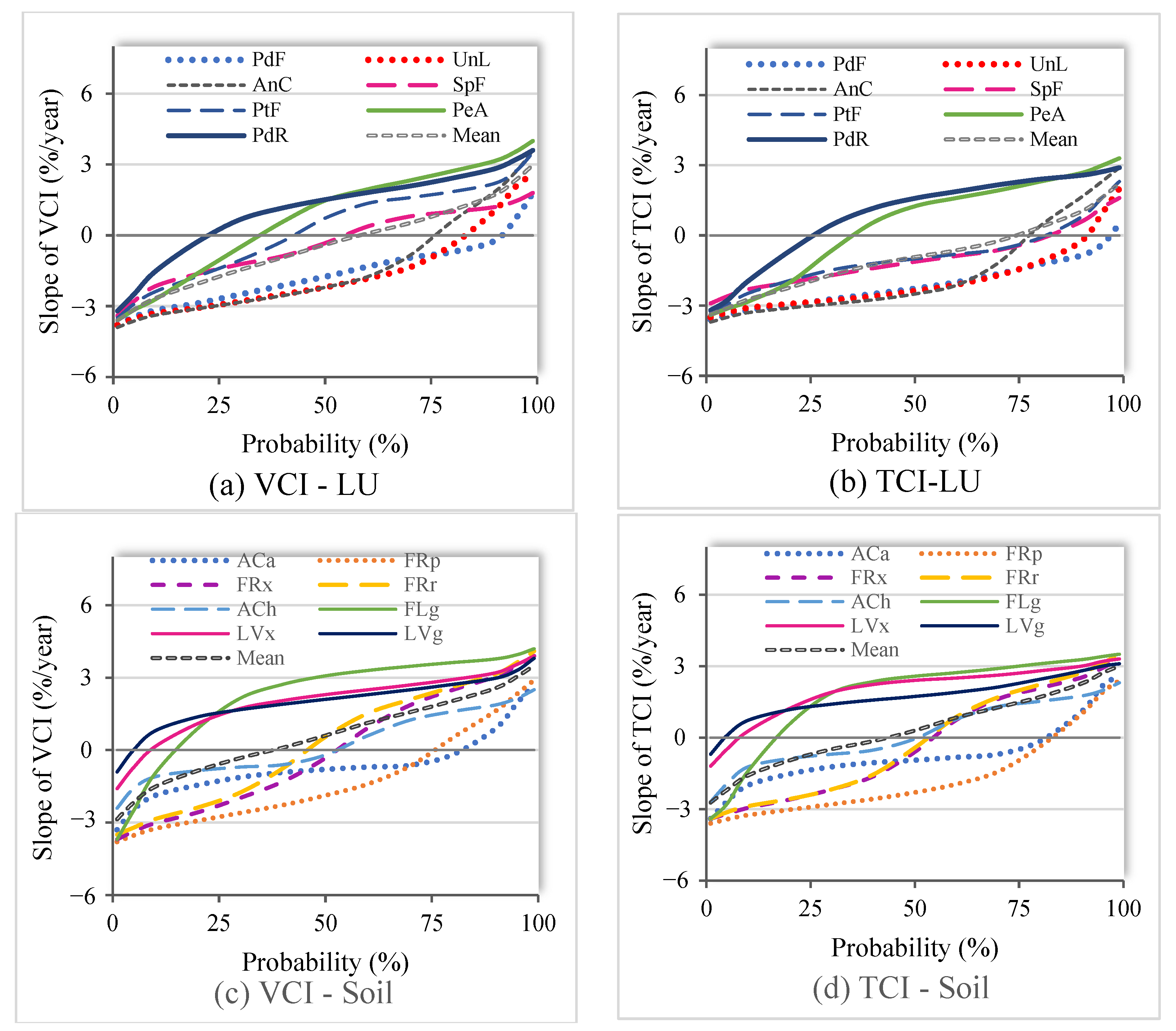
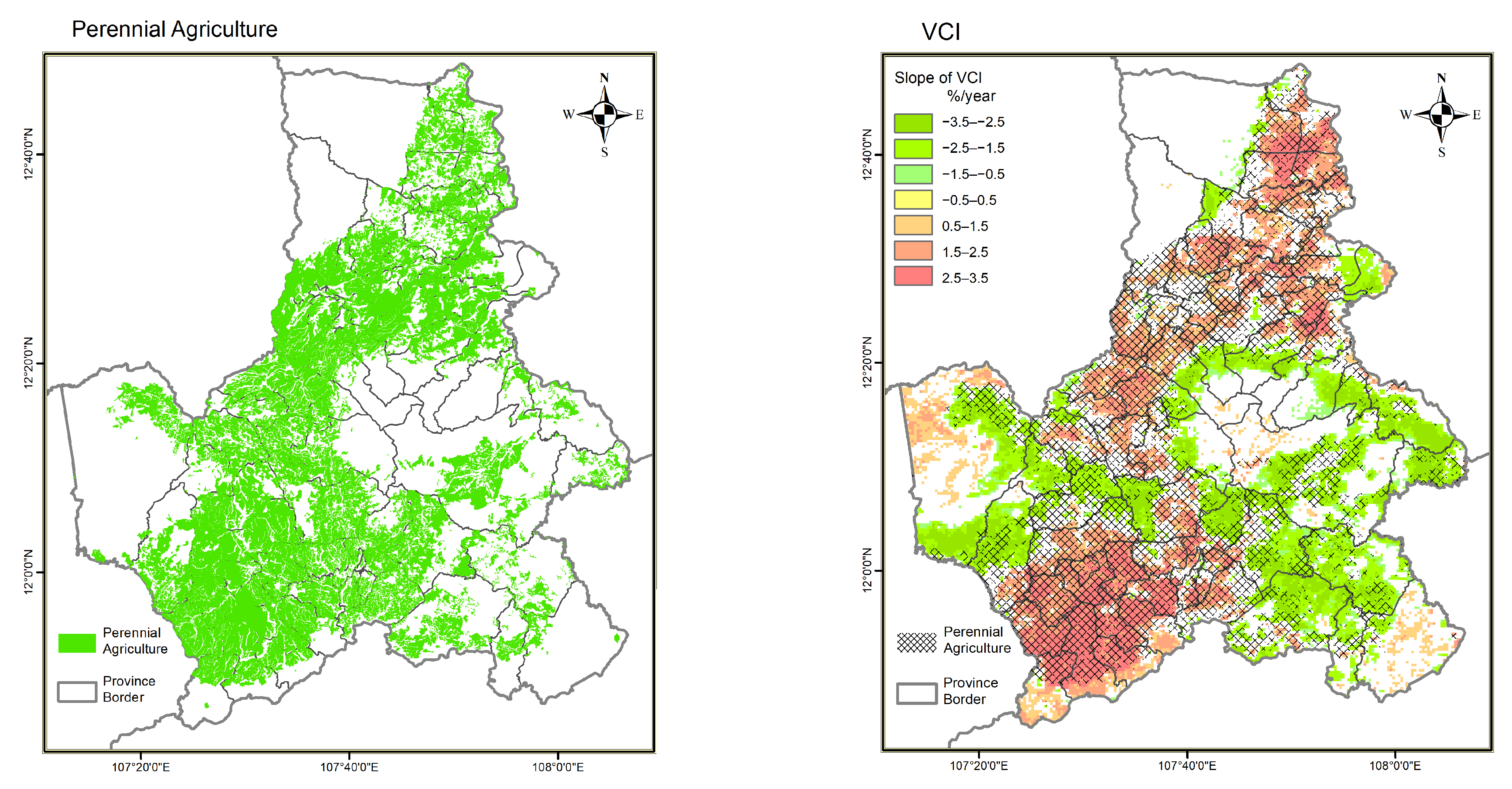
Statistical results of the VHIs’ change based on land use types and soil types are shown in Figure 4. Figure 5 illustrates the overlap between the Perennial Agriculture (PeA) and the VCI’s trend for this statistic. Statistical results in Figure 4 are based on grid cells with a clear trend at a significance level (p = 0.01).
The trend of the VHIs by land use types shown in Figure 4a,b shows three land use groups with different trends. Group 1 includes Paddy Rice (PdR) and PeA; this group tends to increase the VHIs mainly. Compared with the reduced area, the increased area is about two times higher for PeA and three times for PdR. Group 2 included Production Forest (PdF), Unused Land (UnL) and Annual Crops (AnC); this group shows that the VHIs’ decreasing trend is the main one. Compared with the increased area, the reduced area is higher by three times. Group 3 includes Protection Forest (PtF) and Special-use Forest (SpF); the VCI of this group changes a little over time, and the ratio of the increased and decreased area is nearly equal.
The comparison between Figure 4a,b indicates a difference between VCI’s and TCI’s trends in land cover form as PtF. Figure 4a shows an increasing VCI trend on PtF; meanwhile, Figure 4b shows a decreasing trend. Moreover, comparing the lines showing the average values in these figures shows that TCI has mainly a decreasing trend; meanwhile, VCI has nearly similarly an increase and decrease trend.
Figure 4a,b show that in the land use types where humans caused stronger influences on vegetation, there is a clear trend of the VHIs and vice versa. PdF and PeA account for 24% and 38% of the primary land use types. These two types of land use are also controlled by humans and have a clear trend; the downward trend is mainly on PdF, and the increasing trend is mainly on PeA. With PdF, the ratio of the reduced area to area with clear trends is above 90%. With PeA, the ratio of increased area to area tends to be nearly 70% with both VCI and TCI.
Figure 4c,d show that there are three soil types with different VHIs’ trends for soil types. Group 1 shows the mainly increasing VHIs’ trends, including soil types such as Gleyic Luvisols (LVg), Chromic Luvisols (LVx) and Gleyic Fluvisols (FLg). In this group, increasing areas account for over 80%. Group 2 includes Arenic Acrisols (Aca) and Plinthic Ferralsols (FRp). That is the group with a marked decrease in the VHIs, and decreasing areas account for 75% of the total clear trends area. Group 3 includes Xanthic Ferralsols (FRx), Rhodic Ferralsols (FRr) and Haplic Arenosols (Ach). Compared with the above two groups, the trends of this group are less evident in the increasing area, and the decreasing area is almost equal. The comparison between Figure 4c,d shows that in the same soil type, the distribution curve corresponding to TCI is usually lower than VCI. In other words, TCI tends to decrease more than VCI.
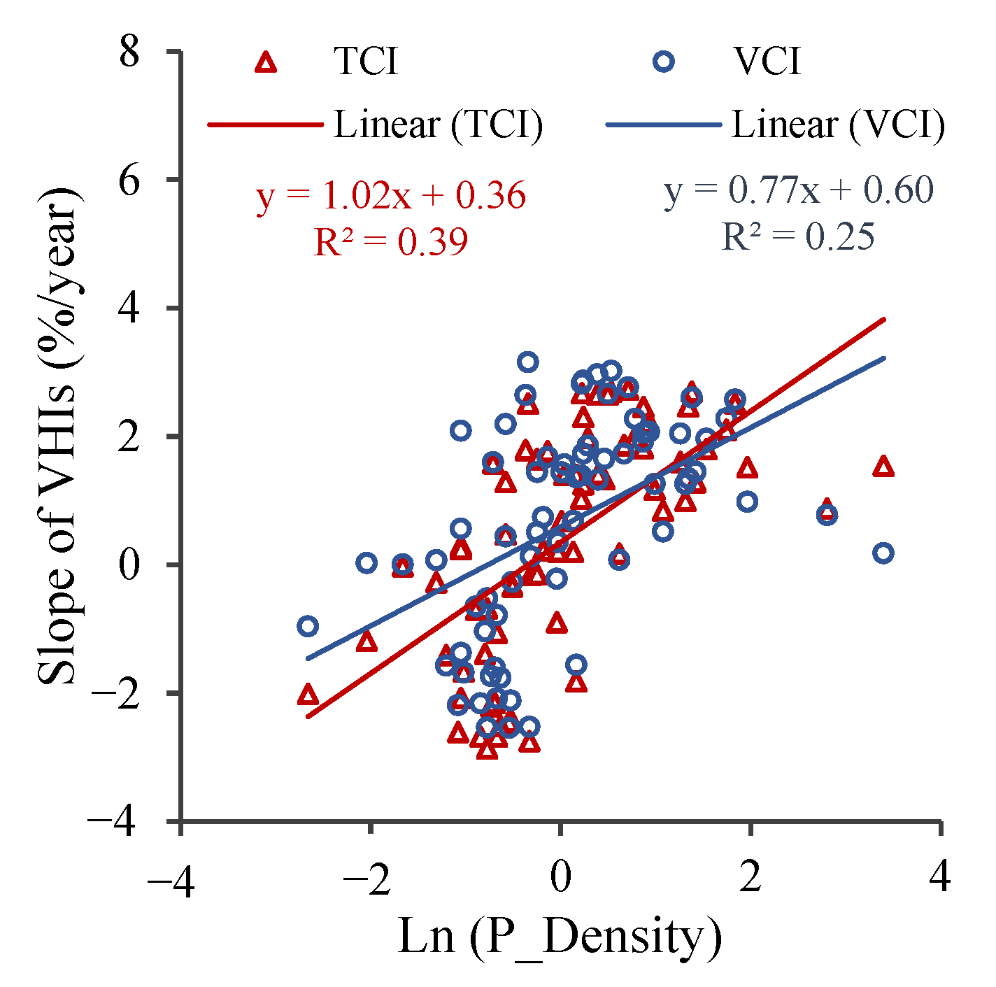
The relationship between the VHIs’ trends and the population density of 71 communes are shown in Figure 6. In this figure, the horizontal axis is a population density’s logarithm in person/ha. The figure shows that the trends of VCI and TCI have a good relationship with population density. Compared with the VCI, TCI is more sensitive to population density changes. Population density is a factor associated with natural and social condition characteristics. The regions have a high population density where, usually, there is a favourable condition for water resources, easily arable land, flat terrain and convenient transportation conditions. These factors are related to the VHIs’ trends and will be considered in the next section.
The preliminary results show that TCI may be more sensitive in assessing vegetation health as it shows a good relationship between population density and a clear trend area larger than VCI. Moreover, compared with VCI, TCI’s trend tends to be more negative. These differences relate to the sensor’s sensitivity and increasing temperature due to climate change, along with the arid conditions of this area during the dry season. Climate change manifests in several ways; it includes an increasing temperature in air and surface. When temperature increases, the amount of evaporation will increase, which causes a shortage of soil moisture in the dry season and limits the photosynthesis process and vegetation growth [1]; this is the cause that contributes to decreasing TCI.

3.2. Determine the Role of Land Use and Soil in the VHIs’ Trend by Logistic Regression Analysis

In this study, the dependent variable is converted to binary form with values of zero and one, showing that the VHIs tend to increase or decrease. With this dependent variable, the logistic regression method is used to evaluate the contribution of factors affecting the VHIs’ trend.
The analysis includes many influencing variables to assess their contribution to the VHIs’ trend. These variables include land use, soil, terrain elevation and slope, population density and growth rate, distance from rivers and distance from roads. Influencing variables have different properties; some are qualitative and some are quantitative and different measurements. Therefore, different methods are used to understand the contribution of each variable in this study. Thus, the logistic regression method was used to determine the role of the categories of the variables, land use and soil, on the VHIs’ trend.

3.2.1. Contribution of Land Use Types or Soil Types to the Trend of VHIs through Logistic Regression Equation

In order to understand the role of land use categories and soil types in VHIs’ trend, a logistic regression equation was built separately for each variable, which are land use and soil. Protection Forest was used as the reference land use category for the land use variable because of its vegetation cover stability over time. For the soil type variable, the reference soil type is Chromic Luvisols, which is the nutrient soil at the average level of this area.
The sequence length for analysis in this study is over 18.000, which is also the number of grid cells with a clear VHIs’ trend. Among these grid cells, half are used for training and the rest for evaluating the prediction equation’s quality. The results of determining the coefficients of the logistic regression equation simulating the VHIs’ trend according to land use or soil types are shown in Table 3. This table shows that according to the decreasing exp(b)’s value, the order of land use and soil types is uniform according to both dependent variables, VCI and TCI.
In this table, exp(b) represents the ratio of the area having an increasing trend and decreasing trend of any land use (or soil) over the ratio of reference land use (or soil). When the values of the analytic variables increase by one unit, the ratio of the area between the increasing and decreasing trend will change several times, equal to its exp(b)’s value. When exp(b) is less than one, it shows the effect of making the VHIs tend to decrease and vice versa in the case of greater than one.
Table 3 shows that the level of influence of land use types on the trend of the VHIs in ascending order from negative to positive would be from Production Forest, Unused Land, Annual Crops, Special-use Forest, Protection Forest, Perennial Agriculture and then to Paddy Rice.
According to Measho et al. [35] and Ghoneim [43], the response of different land cover categories differs from external influences. Comparing the magnitude of exp(b) between the dependent variables, the VHIs’ trend in land use categories shows that except for Special-use Forest, when the independent variables change, the trend of TCI will change more than VCI; in other words, the TCI tendency is to be more sensitive to changes in land use.
With the dependent variables being soil, exp(b) values in the table and reference soil type is Chromic Luvisols; the order according to the influence of soil types on the VHIs’ trend is gradually increasing from negative to positive. The increasing trend would be Arenic Acrisols, Plinthic Ferralsols, Xanthic Ferralsols, Rhodic Ferralsols, Haplic Arenosols, Chromic Luvisols, Gleyic Fluvisols and then Gleyic Luvisols. Changes of the soil characteristics of soil types lead to the change of the VHIs.
There was no significant difference in the coefficients of the logistic regression equation in the VHIs’ trend simulation using the soil variable. However, the opposite would happen if the land use variable was used. This result shows that TCI is much more sensitive than VCI to changes in land use categories. The accuracy in Table 3 is based on the test data series. This result shows that when using only one predictor variable, the quality of the regression equation is low. This result also shows that compared with VCI, the reliability of the equation corresponding to TCI is higher.

3.2.2. The Role of Land Use on the VHIs’ Trend

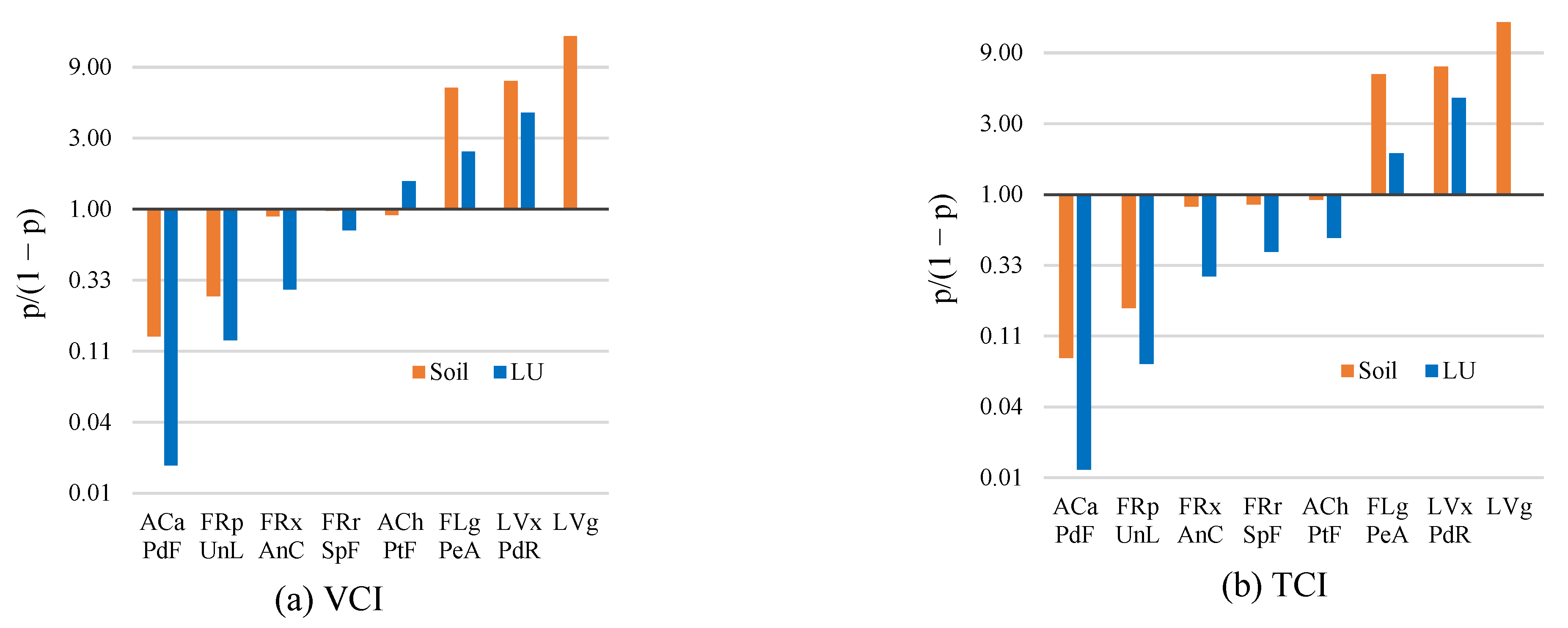
As shown in Figure 7, the VHIs’ trend is very different among land use categories. The VHIs increased markedly on land use forms Perennial Agriculture and Paddy Rice and decreased markedly on land use forms Production Forest, Unused Land and Annual Crops. In the remaining land use types, the trend of the VHIs is not obvious. The increasing trend of the VHIs on Perennial Agriculture and Paddy Rice acreage is clearly due to its favourable location for care, such as proximity to roads and surface water sources, the slight slope of topography and adequate labour resources, which occurs in contrast to Production Forest, Unused Land and Annual Crops (Table 4). This figure also demonstrates that compared to VCI, the trend of TCI tends to be more negative.
In addition, the VHIs increased in Perennial Agriculture and Paddy Rice areas due to investments in seed, fertilizer, irrigation and mechanization in agriculture. According to Müller and Zeller [6], after 1992, Perennial Agriculture and Paddy Rice rapidly developed, relying on migrant labour, increased capital and fertilizer, improved access to rural roads and markets and expanded coverage of irrigated areas. According to data from the General Statistics Office of Vietnam in Dak Nong province, from 2000 to 2020, rice yield increased by 0.07 tons/ha/year, and coffee yield increased by 0.03 tons/year/ha. Combined with forest protection and discouraging shifting cultivation policies, forest cover stabilized after 1992. That is the reason that the trend of the VHIs is not apparent in the Protection Forest and Special-use Forest. The decline of the VHIs on land use types is in the Production Forest, Unused Land and Annual Crops, in addition to the disadvantages mentioned above, due to their low economic efficiency; consequently, it is not invested. Combined with inadequate rainfall during the dry season and the increase in temperature due to climate change, it has caused the trend of the VHIs on these land uses to decrease.

3.2.3. The Role of Soil Types on the VHIs’ Trend

Similar to land use, the VHIs’ trend also shows a clear association with soil types (Figure 7). The decline of the VHIs was evident on Arenic Acrisols and Plinthic Ferralsols soils and increased markedly on Gleyic Fluvisols, Chromic Luvisols and Gleyic Luvisols soils. In the remaining soil types, the trend of the VHIs is not obvious. The difference in the VHIs’ trend on soil types is related to soil nutrients, in which Arenic Acrisols and Plinthic Ferralsols are nutrient-poor soils compared to Gleyic Fluvisols, Chromic Luvisols and Gleyic Luvisols soils.
According to Donohue et al. [44], vegetation cover can also be declined on nutrient-rich soil and easily degraded due to soil erosion and poor field management. In addition to the nutrient issue, the difference in the VHIs’ trend in these two soil types is also due to (1) differences in vegetation on soil types, and (2) differences in population density by soil types and location of soil types relative to surface water sources and roads.
On the soil types of Arenic Acrisols and Plinthic Ferralsols, the area ratio of the Production Forest and Annual Crops group to the Perennial Agriculture and Paddy Rice group has values of 5.24 and 1.62, respectively. However, for soil types Gleyic Fluvisols, Chromic Luvisols and Gleyic Luvisols, this ratio is only 0.12, 0.76 and 0.45, respectively. Since this is the ratio of the area between the vegetation groups with decreased and increased VHIs, it shows that one of the reasons of the difference in the VHIs’ trend in soil types is related to land use.
Table 4 shows that compared with Arenic Acrisols and Plinthic Ferralsols, the remaining soil types have a higher population density, closer to surface water sources and roads. Therefore, where there is poor soil, there is a shortage of labour resources, difficulty to access and a lack of surface water. Combined with the increase in irrigation requirements due to climate change and that the economic profit is low in these places, it has been cut off in investment to focus on other economic activities, making the VHIs tend to be more declined. In contrast to Arenic Acrisols and Plinthic Ferralsols, the remaining soil types have favourable cultivation locations and abundant labour resources.
The land use types of Production Forest, Unused Land and Annual Crops and soil types of Arenic Acrisolsand Plinthic Ferralsols are quite far from surface water sources (Table 4) and are where the VHIs have decreased sharply (Figure 7). According to the research results of Luong [41], there is negligible rainfall in this area during the dry season, combined with a temperature increase of 0.03 °C/year or 0.6 °C in the past 20 years, which has increased the demand for irrigated crops and increased drought conditions. Therefore, the area far from the surface water sources increases the lack of water for crops during dry seasons, which decreases the VHIs.
The influence of the combination between land use and soils on the VHIs’ trend is shown in Figure 8. The result shows that the areas of land use types of Production Forest and Annual Crops and soil types of Arenic Acrisols and Plinthic Ferralsols have decreased the VHIs’ trend mainly, with the clear trend area accounting for 92%. On the other hand, for the land use types of Perennial Agriculture and Paddy Rice and soil types of Chromic Luvisols and Gleyic Luvisols, areas with an increased VHIs’ trend are the main areas, with clear trend areas accounting for 95%. In addition, this figure illustrates that VCI tends to decrease more than TCI.

3.3. The Role of Influence Factors on the VHIs’ Trend by Discriminant Analysis

Similar to logistic regression analysis, in this analysis, independent variables are in binary form to show the increase or decrease trends of the VHIs. Eight influence variables are used in the analysis, including land use (LU), soil, elevation, slope, population density (P_Density), population growth rate (P_Rate), distance from the river (D_River) and distance from roads (D_Roads). When using discriminant analysis, independent variables need to convert to quantitative form and the same measure.

3.3.1. Convert Independent Variables to Ratio Scale

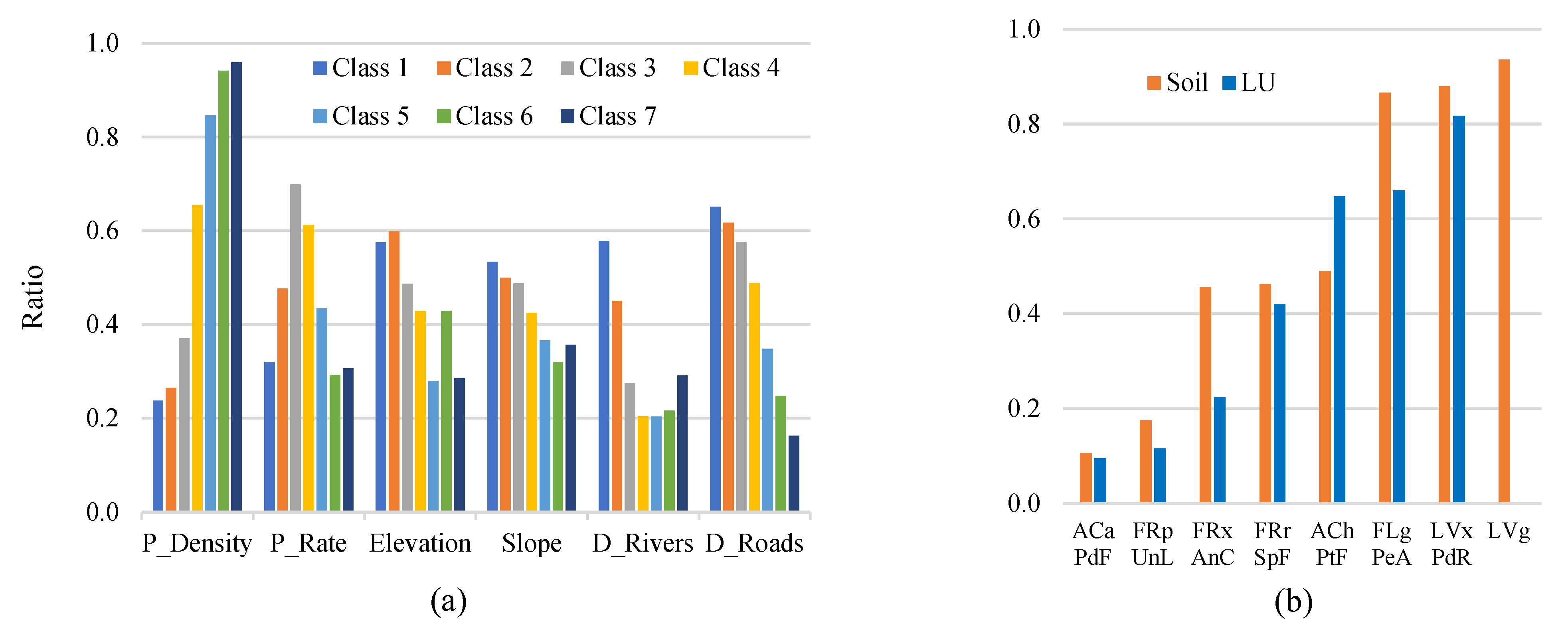
In this study, converting to create the new variables is done as follows: (1) with continuous independent variables (except LU and soil), divide into groups according to value ranges; and (2) with each independent variable, calculate the ratio of the area where the VHIs tend to increase to the area with a clear trend corresponding with divided groups or land use types and soil types; these values are used as values of new variables. In step 1, continuous variables were divided into seven classes with thresholds shown in Table 5. These thresholds were determined by testing gradually until the accuracy of the discriminant function was the highest. In step 2, due to no significant difference between the calculated results for VCI and TCI, their average values were taken as the value of new variables. These values are shown in Figure 9. Therefore, afterwards, these changing, independent variables were converted to the same measure and have values between zero and one.

3.3.2. The Role of Independent Variables on the VHIs’ Trend through Standardized Coefficients of Discriminant Function

With the data series length being over 18.000, it was divided randomly into two parts, one for training and the rest for testing, besides assessing and testing based on the method “Leave one out classification”. This method built a discriminant function based on the distance of Mahalanobis; the stepwise method is used to select variables for analysis.
The standardized coefficients of the discriminant function and structure matrix according to a step by step are shown in Table 6. According to the structure matrix in this table, coefficients of the discriminant function are determined in step 2. In this step, all variables participating in the discriminant function meet the reliability; however, due to the relatively small, standardized coefficient corresponding to the D_River variable in the VCI of the discriminant function, this variable can be eliminated. Table 7 presents coefficients and the accuracy of the discriminant function based on an independent test series. The accuracy of using the method “Leave one out classification” is not presented because it gives a higher accuracy than the independent series test method.
This result shows that for both VCI and TCI, the order of contribution to the difference gradually decreases from P_Density, LU, soil, P_Rate and D_Roads, particularly for TCI in the discriminant function added into the variable D_Rivers; this variable had the lowest contribution. The elevation and slope variables do not contribute to the difference; these are natural variables and almost unchanged over time. Among the selected variables, soil is a natural variable; however, this variable also changes over time, such as changes in nutritional composition.
According to Table 7, compared with VCI, the magnitude of the coefficients of the discriminant function corresponding to TCI are higher, and the clearest is P_Density. This result illustrates that TCI will be easier to change than VCI when variables in this equation change, and the most sensitive to change is P_Density. In addition, the accuracy of the discriminant function corresponding to TCI is also higher than VCI, showing that using TCI in vegetation health monitoring is a priority option.

3.3.3. Analysing the Role of Independent Variables on the VHIs’ Trend

Independent variables were discussed, including variables participating in the logistic regression equation in Table 7, including P_Density, LU, soil, P_Rate and then D_Roads, in which the roles of LU and soil variables were analyzed above.
  • Population density (P_Density);
According to Figure 9a, except for topographic elevation, slope and distance from rivers, the areas with an increased VHIs’ trend significantly differ by class. The most apparent difference is the population density variable. For this variable, the area with an increased VHIs’ trend is nearly proportional to population density. Places with population densities above 1.8 people/ha have the most significant increase in VHIs, whereas places with population densities below 0.5 people/ha have VHIs that tend to increase clarity. High population density reflects the meeting for human sources for crop care. Population density is also related to factors such as land use, soil, water sources and others, which are also related to vegetation cover.
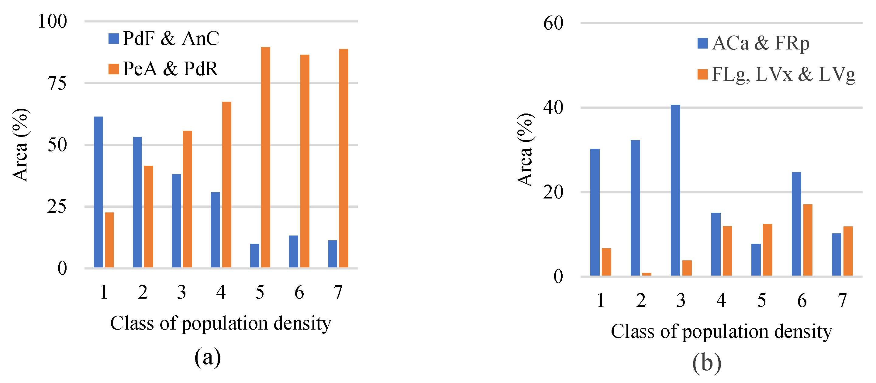
There are 94% of the population in this area, concentrated in four main land use types, including Production Forest, Annual Crops, Perennial Agriculture and Paddy Rice. According to Figure 10a, places have high population densities mainly concentrated in Perennial Agriculture and Paddy Rice; these plant groups have increased the VHIs’ trends. In contrast, in places with low population densities mainly concentrated in Production Forest and Annual Crops, these plant groups have decreased the VHIs’ trends. According to Figure 10b, places with high population densities are places where soil types significantly increase the VHIs’ trends and vice versa. These figures show the relationship between population density, crop types, soil types and the VHIs’ trend.
  • Population growth rate;
The relationship between the VHIs’ trend and population growth rate is shown in Figure 9a. Combined with Table 5, it is shown that P_Rates below 0.6%/year or above 4.6%/year are associated with decreased VHIs. Communes with a P_Rate of less than 0.6%/year are the communes with low P_Density, or places with low labour sources for farming and have soil types and land use types of places with a low population where the VHIs’ trends decrease. Furthermore, localities with a P_Rate of over 4.5%/year show a high urbanization rate or a part of the plant area will be converted into construction land and reduce the VHIs.
  • Distance from roads;
As shown in Figure 9a, the distance from the cultivated land to roads is proportional to the VHIs’ trend. This figure showed that compared with the P_Rate, elevation, slope and D_Rivers variables, the VHIs are more sensitive than these variables. Distance from roads represents the convenience of access to crop care, the possibility of agricultural mechanization, the purchase and sale of agricultural materials and the sale of harvest production. These advantages lead to higher profits and better crop care based on these profit sources. The road system is not a stable element, but it can change over time through freight traffic increase; the road was widened or made new; therefore, if in the same natural condition, crops in convenient traffic places will have the VHIs increase and vice versa in inconvenient places.
Besides the advantage from roads, according to Table 4, Perennial Agriculture and Paddy Rice are grown near roads. These crops have a significant increase in the VHIs’ trend. Moreover, this result shows that the main soil types near the road are Gleyic Fluvisols, Chromic Luvisols and Gleyic Luvisols, with a clearly increased trend of the VHIs. These characteristics contribute to the VHIs’ trend increase in places near the roads.
  • Distance from rivers.
The magnitude of the coefficients of the discriminant function corresponding to the D_River variable in Figure 7 shows that the contribution of this variable is not significant to the VHIs’ trend. The reason can be that D_Rivers is a natural variable and relatively unchanged over time; therefore, the contribution of this variable is not considerable. However, this variable is a factor representing the ability to supply water to crops; thus, in the places where water shortages are increasing due to climate change, the VHIs’ trends may reduce. Moreover, high temperatures due to climate change and low soil moisture due to lack of irrigation water during dry seasons increased water stress levels, making plants underdeveloped (Kogan [34]) or causing reduced VHIs. In addition, in Table 4, places near the river also have crop and soil types with increased VHIs’ trends. These characteristics contribute to increasing the VHIs’ trends in places near surface water. The above results show that several factors clearly influence the trend of the VHIs that humans can change to increase cover, such as rising roads and population in low-density areas. In addition, this result also shows that the land use type should be something other than production forest or fallow land on nutrient-poor soils.

3.3.4. Accuracy of Simulation Results According to Predictor Variables

This step aims to initially identify the causes related to the quality of the trend simulation of the VHIs using the discriminant analysis method. Figure 11 shows the accuracy of the simulation results, where the black points represent the incorrect simulation, and the remaining colour shows the correct result. This result shows that the distribution of points with true and false results is relatively similar between VCI and TCI, and the incorrect part is not scattered but concentrated in some places.
The assessment of the trend forecasting accuracy of the VHIs according to the influencing factors will be based on this distribution. The variables included in the analysis appear in the discriminant function, as shown in Table 7. For the variables P_Density, P_Rate, D_Roads and D_Rivers, the analysis of the accuracy of the simulation results is based on the classes divided in Table 5. For the LU and soil variables, the accuracy is statistically calculated according to soil and land use types; the statistical results are shown in Figure 12.
Figure 12 shows that only three variables, P_Density, LU and soil, have significant differences in the accuracy of simulation results according to soil types, LU and population density classes. According to Figure 9, these are also the variables with the ratio of the area where the VHIs tend to increase to the apparent trend area with the largest amplitude.
With P_Density, low precision corresponds to a place with medium population density and high corresponds to a very high or very low population density. Population density and population growth have affected the VHIs’ trend as analyzed; when these data are stable, the VHIs are less changing and are accurate in simulating the VHIs’ trends which will be lower and vice versa when these data are unstable.
With LU, the accuracy of the discriminant function is relatively low when the land use types are Special-use Forest and Protection Forest. It can be explained as with P_Density, because Special-use Forest and Protection Forest are land use types with less change over time. A Protection Forest related to hydroelectric reservoir systems is strictly protected and less impacted by humans. Moreover, due to its location near water sources, the influences of climate change on water requirements here are not obvious. These characteristics made the VHIs in the Protection Forest have less change over time, and its ability to simulate up and down trends is with low accuracy. In contrast to Special-use Forest and Protection Forest, the accuracy of the discriminant function with Production Forest, Unused Land and Paddy Rice has the highest accuracy because these are the land use types with a significant change in land cover, for the reasons indicated.
Similar to the variables LU and P_Density, because on the soil types including Arenic Acrisols, Plinthic Ferralsols, Chromic Luvisols and Gleyic Luvisols there is a strong tendency of VHIs, the accuracy of the discriminant function will be high. In contrast, the accuracy will be low on the soil types where the VHIs’ trend is unclear such as Xanthic Ferralsols and Rhodic Ferralsols.
Figure 5 and Figure 8 show that the discriminant function’s accuracy will be high in the clear trend area and vice versa. High-accuracy areas are characterized as densely or over-populated on Arenic Acrisols, Plinthic Ferralsols, Chromic Luvisols and Gleyic Luvisols soils and Production Forest, Unused Land and Paddy Rice land use types. Conversely, the low-precision areas were moderately densely populated on Xanthic Ferralsols and Rhodic Ferralsols soils and Special-use Forest and Protection Forest land use categories.

4. Conclusions

This study shows that both VCI and TCI have apparent trends in the dry season and show both increase and decrease tendencies. The distribution of grid cells with increasing and decreasing trends of VCI and TCI is relatively the same. With VCI, the areas with increasing, decreasing and indistinct trends are nearly equivalent. With TCI, the area with a decreasing trend is higher than an increasing area by 1.6 times. The total clear trend area for TCI is higher than VCI. The more negative deviation of TCI compared with VCI is related to the increasing temperature due to climate change, causing a lack of soil moisture in the places away from surface water sources during the dry season.
Significant differences exist in the VHIs’ trends by land use and soil types. The land use types related to the primary income sources from agricultural production, namely Perennial Agriculture and Paddy Rice, have VCI and TCI with significant increasing trends. In contrast, in low economic efficiency soil and land use types, the VHIs tend to decrease. Differences in the trends of the VHIs across soils and land uses are also related to other properties, such as population, water sources, transport and topography.
Based on logistic regression analysis, it is shown that the influence of land use types on the trend of the VHIs in an increasing direction from negative to positive will include from Production Forest, Unused Land, Annual Crops, Special-use Forest, Protection Forest, Perennial Agriculture and then to Paddy Rice. According to the order, when there is an area change at the beginning and the end of the group, the VHIs will change markedly. For soil, the influence of soil types on the trend of the VHIs in the direction of increasing from negative to positive will include from Arenic Acrisols, Plinthic Ferralsols, Xanthic Ferralsols, Rhodic Ferralsols, Haplic Arenosols, Chromic Luvisols, Gleyic Fluvisols and then Gleyic Luvisols. This result also shows that production forests should not be planted or bear on nutrient-poor soils to increase the cover.
Based on the discriminant analysis method, it was found that there are only four primary factors affecting the VHIs’ trend in order to decrease gradually, including population density, land use, soil, population growth rate and distance from the road. The role of the variables in this order relates to human resources, priority in crop cultivation and changes in seeds and farming methods. Based on this result, it is possible to adjust one of these factors for plant growth.
The coefficients of the logistic regression equation and the discriminant function illustrate that the TCI is more sensitive than the VCI when the independent variables change, especially for changes in population density and land use. Furthermore, the correlation coefficient analysis results between the trend of VCI or TCI with population density show a good relationship, and TCI has a higher correlation coefficient than VCI. Therefore, TCI can be considered a priority choice in assessing the trend of vegetation health during the dry time in the context of climate change.

Author Contributions

Conceptualization, L.V.V., N.T.T.T. and N.V.H.; methodology, L.V.V., N.T.T.T. and N.V.H.; analysis, N.V.H. and L.V.V.; writing—original draft, N.T.T.T., N.V.H. and L.V.V.; writing—review and editing, N.T.T.T., L.V.V., N.V.H., H.C.L. and L.H.B. All authors have read and agreed to the published version of the manuscript.

Funding

This research received no external funding.

Institutional Review Board Statement

Not applicable.

Informed Consent Statement

Not applicable.

Data Availability Statement

The in situ datasets generated and/or analyzed during the current study and the satellite derived database are available from the corresponding author upon reasonable request. The geographical boundaries of the fields analyzed during the current study are not publicly available due to privacy protection. The satellite images are freely available at https://earthexplorer.usgs.gov/).

Acknowledgments

The authors thank the Dak Nong province for supplying data. Population data were collected for each commune in Dak Nong province. Soil and land use data were obtained from the Department of Agriculture and Rural Development of Dak Nong province. Satellite data were from the United States Geological Survey website (source: https://earthexplorer.usgs.gov/) (accessed on 25 October 2022).

Conflicts of Interest

The authors declare no conflict of interest.

References

  1. Yang, Y.; Wang, S.; Bai, X.; Tan, Q.; Li, Q.; Wu, L.; Tian, S.; Hu, Z.; Li, C.; Deng, Y. Factors Affecting Long-Term Trends in Global NDVI. Forests 2019, 10, 372. [Google Scholar] [CrossRef] [Green Version]
  2. Cao, M.; Woodward, F.I. Dynamic responses of terrestrial ecosystem carbon cycling to global climate change. Nature 1998, 393, 249–252. [Google Scholar] [CrossRef]
  3. Liu, X.F.; Zhu, X.F.; Pan, Y.-Z.; Li, Y.Z.; Zhao, A.Z. Spatiotemporal Changes in Vegetation Coverage in China during 1982–2012. Shengtai Xuebao/Acta Ecol. Sin. 2015, 35, 5331–5342. [Google Scholar] [CrossRef]
  4. Chen, C.; Park, T.; Wang, X.; Piao, S.; Xu, B.; Chaturvedi, R.K.; Fuchs, R.; Brovkin, V.; Ciais, P.; Fensholt, R.; et al. China and India Lead in Greening of the World through Land-Use Management. Nat. Sustain. 2019, 2, 122–129. [Google Scholar] [CrossRef]
  5. Rehman, A.; Qin, J.; Shafi, S.; Khan, M.S.; Ullah, S.; Ahmad, K.; Rehman, N.U.; Faheem, M. Modelling of Land Use/Cover and LST Variations by Using GIS and Remote Sensing: A Case Study of the Northern Pakhtunkhwa Mountainous Region, Pakistan. Sensors 2022, 22, 4965. [Google Scholar] [CrossRef] [PubMed]
  6. Müller, D.; Zeller, M. Land Use Dynamics in the Central Highlands of Vietnam: A Spatial Model Combining Village Survey Data with Satellite Imagery Interpretation. Agric. Econ. 2002, 27, 333–354. [Google Scholar] [CrossRef]
  7. Da Silva Melo, M.R.; Rocha, J.V.; Manabe, V.D.; Lamparelli, R.A.C. Intensity of Land Use Changes in a Sugarcane Expansion Region, Brazil. J. Land Use Sci. 2018, 13, 182–197. [Google Scholar] [CrossRef]
  8. Tomasella, J.; Silva Pinto Vieira, R.M.; Barbosa, A.A.; Rodriguez, D.A.; de Oliveira Santana, M.; Sestini, M.F. Desertification Trends in the Northeast of Brazil over the Period 2000–2016. Int. J. Appl. Earth Obs. Geoinf. 2018, 73, 197–206. [Google Scholar] [CrossRef]
  9. Singh, R.P.; Roy, S.; Kogan, F. Vegetation and Temperature Condition Indices from NOAA AVHRR Data for Drought Monitoring over India. Int. J. Remote Sens. 2003, 24, 4393–4402. [Google Scholar] [CrossRef]
  10. Thao, N.T.T.; Khoi, D.N.; Denis, A.; Van Viet, L.; Wellens, J.; Tychon, B. Early Prediction of Coffee Yield in the Central Highlands of Vietnam Using a Statistical Approach and Satellite Remote Sensing Vegetation Biophysical Variables. Remote Sens. 2022, 14, 2975. [Google Scholar] [CrossRef]
  11. Kriegler, F.J.; Malila, W.A.; Nalepka, R.F.; Richardson, W. Preprocessing Transformations and Their Effect on Multispectral Recognition. Remote Sens. Environ. 1969, 6, 97–132. [Google Scholar]
  12. Huang, S.; Tang, L.; Hupy, J.P.; Wang, Y.; Shao, G. A Commentary Review on the Use of Normalized Difference Vegetation Index (NDVI) in the Era of Popular Remote Sensing. J. For. Res. 2021, 32, 1–6. [Google Scholar] [CrossRef]
  13. Baret, F.; Guyot, G. Potentials and Limits of Vegetation Indices for LAI and APAR Assessment. Remote Sens. Environ. 1991, 35, 161–173. [Google Scholar] [CrossRef]
  14. Bannari, A.; Morin, D.; Bonn, F.; Huete, A.R. A Review of Vegetation Indices. Remote Sens. Rev. 1995, 13, 95–120. [Google Scholar] [CrossRef]
  15. Wang, X.; Piao, S.; Ciais, P.; Li, J.; Friedlingstein, P.; Koven, C.; Chen, A. Spring Temperature Change and Its Implication in the Change of Vegetation Growth in North America from 1982 to 2006. Proc. Natl. Acad. Sci. USA 2011, 108, 1240–1245. [Google Scholar] [CrossRef] [PubMed] [Green Version]
  16. Tucker, C.J.; Pinzon, J.E.; Brown, M.E.; Slayback, D.A.; Pak, E.W.; Mahoney, R.; Vermote, E.F.; El Saleous, N. An Extended AVHRR 8-Km NDVI Dataset Compatible with MODIS and SPOT Vegetation NDVI Data. Int. J. Remote Sens. 2005, 26, 4485–4498. [Google Scholar] [CrossRef]
  17. Tian, J.; Wang, L.; Li, X.; Gong, H.; Shi, C.; Zhong, R.; Liu, X. Comparison of UAV and WorldView-2 Imagery for Mapping Leaf Area Index of Mangrove Forest. Int. J. Appl. Earth Obs. Geoinf. 2017, 61, 22–31. [Google Scholar] [CrossRef]
  18. Zhu, X.; Liu, D. Improving Forest Aboveground Biomass Estimation Using Seasonal Landsat NDVI Time-Series. ISPRS J. Photogramm. Remote Sens. 2015, 102, 222–231. [Google Scholar] [CrossRef]
  19. Pastor-Guzman, J.; Atkinson, P.M.; Dash, J.; Rioja-Nieto, R. Spatiotemporal Variation in Mangrove Chlorophyll Concentration Using Landsat 8. Remote Sens. 2015, 7, 14530–14558. [Google Scholar] [CrossRef] [Green Version]
  20. Chávez, R.O.; Clevers, J.G.P.W.; Decuyper, M.; de Bruin, S.; Herold, M. 50 Years of Water Extraction in the Pampa Del Tamarugal Basin: Can Prosopis tamarugo Trees Survive in the Hyper-Arid Atacama Desert (Northern Chile)? J. Arid Environ. 2016, 124, 292–303. [Google Scholar] [CrossRef]
  21. Vicente-Serrano, S.M.; Camarero, J.J.; Olano, J.M.; Martín-Hernández, N.; Peña-Gallardo, M.; Tomás-Burguera, M.; Gazol, A.; Azorin-Molina, C.; Bhuyan, U.; El Kenawy, A. Diverse Relationships between Forest Growth and the Normalized Difference Vegetation Index at a Global Scale. Remote Sens. Environ. 2016, 187, 14–29. [Google Scholar] [CrossRef] [Green Version]
  22. Shuai, J.; Zhang, Z.; Tao, F.; Shi, P. How ENSO Affects Maize Yields in China: Understanding the Impact Mechanisms Using a Process-Based Crop Model. Int. J. Climatol. 2016, 36, 424–438. [Google Scholar] [CrossRef]
  23. Baniya, B.; Tang, Q.; Xu, X.; Haile, G.G.; Chhipi-Shrestha, G. Spatial and Temporal Variation of Drought Based on Satellite Derived Vegetation Condition Index in Nepal from 1982–2015. Sensors 2019, 19, 430. [Google Scholar] [CrossRef] [Green Version]
  24. Moussa Kourouma, J.; Eze, E.; Negash, E.; Phiri, D.; Vinya, R.; Girma, A.; Zenebe, A. Assessing the Spatio-Temporal Variability of NDVI and VCI as Indices of Crops Productivity in Ethiopia: A Remote Sensing Approach. Geomat. Nat. Hazards Risk 2021, 12, 2880–2903. [Google Scholar] [CrossRef]
  25. Imran, H.M.; Hossain, A.; Islam, A.K.M.S.; Rahman, A.; Bhuiyan, M.A.E.; Paul, S.; Alam, A. Impact of Land Cover Changes on Land Surface Temperature and Human Thermal Comfort in Dhaka City of Bangladesh. Earth Syst. Environ. 2021, 5, 667–693. [Google Scholar] [CrossRef]
  26. Tran, D.X.; Pla, F.; Latorre-Carmona, P.; Myint, S.W.; Caetano, M.; Kieu, H.V. Characterizing the Relationship between Land Use Land Cover Change and Land Surface Temperature. ISPRS J. Photogramm. Remote Sens. 2017, 124, 119–132. [Google Scholar] [CrossRef] [Green Version]
  27. Purwanto; Utomo, D.H.; Kurniawan, B.R. Spatio Temporal Analysis Trend of Land Use and Land Cover Change Against Temperature Based on Remote Sensing Data in Malang City. Procedia-Soc. Behav. Sci. 2016, 227, 232–238. [Google Scholar] [CrossRef] [Green Version]
  28. Kogan, F. World Droughts in the New Millennium from Avhrr-Based Vegetation Health Indices. Eos Trans. Am. Geophys. Union 2002, 83, 3–7. [Google Scholar] [CrossRef]
  29. Xue, J.; Su, B. Significant Remote Sensing Vegetation Indices: A Review of Developments and Applications. J. Sensors 2017, 2017, 1353691. [Google Scholar] [CrossRef] [Green Version]
  30. Behrang Manesh, M.; Khosravi, H.; Heydari Alamdarloo, E.; Saadi Alekasir, M.; Gholami, A.; Singh, V.P. Linkage of Agricultural Drought with Meteorological Drought in Different Climates of Iran. Theor. Appl. Climatol. 2019, 138, 1025–1033. [Google Scholar] [CrossRef]
  31. Bento, V.A.; Trigo, I.F.; Gouveia, C.M.; DaCamara, C.C. Contribution of Land Surface Temperature (TCI) to Vegetation Health Index: A Comparative Study Using Clear Sky and All-Weather Climate Data Records. Remote Sens. 2018, 10, 1324. [Google Scholar] [CrossRef] [Green Version]
  32. Henchiri, M.; Liu, Q.; Essifi, B.; Javed, T.; Zhang, S.; Bai, Y.; Zhang, J. Spatio-Temporal Patterns of Drought and Impact on Vegetation in North and West Africa Based on Multi-Satellite Data. Remote Sens. 2020, 12, 3869. [Google Scholar] [CrossRef]
  33. Jiang, R.; Liang, J.; Zhao, Y.; Wang, H.; Xie, J.; Lu, X.; Li, F. Assessment of Vegetation Growth and Drought Conditions Using Satellite-Based Vegetation Health Indices in Jing-Jin-Ji Region of China. Sci. Rep. 2021, 11, 13775. [Google Scholar] [CrossRef]
  34. Kogan, F.N. Operational Space Technology for Global Vegetation Assessment. Bull. Am. Meteorol. Soc. 2001, 82, 1949–1964. [Google Scholar] [CrossRef]
  35. Measho, S.; Chen, B.; Trisurat, Y.; Pellikka, P.; Guo, L.; Arunyawat, S.; Tuankrua, V.; Ogbazghi, W.; Yemane, T. Spatio-Temporal Analysis of Vegetation Dynamics as a Response to Climate Variability and Drought Patterns in the Semiarid Region, Eritrea. Remote Sens. 2019, 11, 724. [Google Scholar] [CrossRef] [Green Version]
  36. NourEldeen, N.; Mao, K.; Yuan, Z.; Shen, X.; Xu, T.; Qin, Z. Analysis of the Spatiotemporal Change in Land Surface Temperature for a Long-Term Sequence in Africa (2003–2017). Remote Sens. 2020, 12, 488. [Google Scholar] [CrossRef] [Green Version]
  37. Song, X.P.; Hansen, M.C.; Stehman, S.V.; Potapov, P.V.; Tyukavina, A.; Vermote, E.F.; Townshend, J.R. Global Land Change from 1982 to 2016. Nature 2018, 560, 639–643. [Google Scholar] [CrossRef]
  38. Pandey, P.C.; Chauhan, A.; Maurya, N.K. Evaluation of Earth Observation Datasets for LST Trends over India and Its Implication in Global Warming. Ecol. Inform. 2022, 72, 101843. [Google Scholar] [CrossRef]
  39. Nzoiwu, C.P.; Agulue, E.I.; Mbah, S.; Igboanugo, C.P. Impact of Land Use/Land Cover Change on Surface Temperature Condition of Awka Town, Nigeria. J. Geogr. Inf. Syst. 2017, 09, 763–776. [Google Scholar] [CrossRef] [Green Version]
  40. Kogan, F.N. Application of Vegetation Index and Brightness Temperature for Drought Detection. Adv. Space Res. 1995, 15, 91–100. [Google Scholar] [CrossRef]
  41. Luong, V.V. Effects of ENSO and Climate Change on Reference Evapotranspiration in Southern Vietnam. J. Meteorol. Res. 2021, 35, 868–881. [Google Scholar] [CrossRef]
  42. Kukunuri, A.N.J.; Murugan, D.; Singh, D. Variance Based Fusion of VCI and TCI for Efficient Classification of Agriculture Drought Using MODIS Data. Geocarto Int. 2022, 37, 2871–2892. [Google Scholar] [CrossRef]
  43. Ghoneim, E. Vegetation Drought Analysis In Tunisia: A Geospatial Investigation. J. Atmos. Earth Sci. 2017, 1, 1–9. [Google Scholar] [CrossRef]
  44. Donohue, R.J.; Mcvicar, T.R.; Roderick, M.L. Climate-Related Trends in Australian Vegetation Cover as Inferred from Satellite Observations, 1981-2006. Glob. Chang. Biol. 2009, 15, 1025–1039. [Google Scholar] [CrossRef]
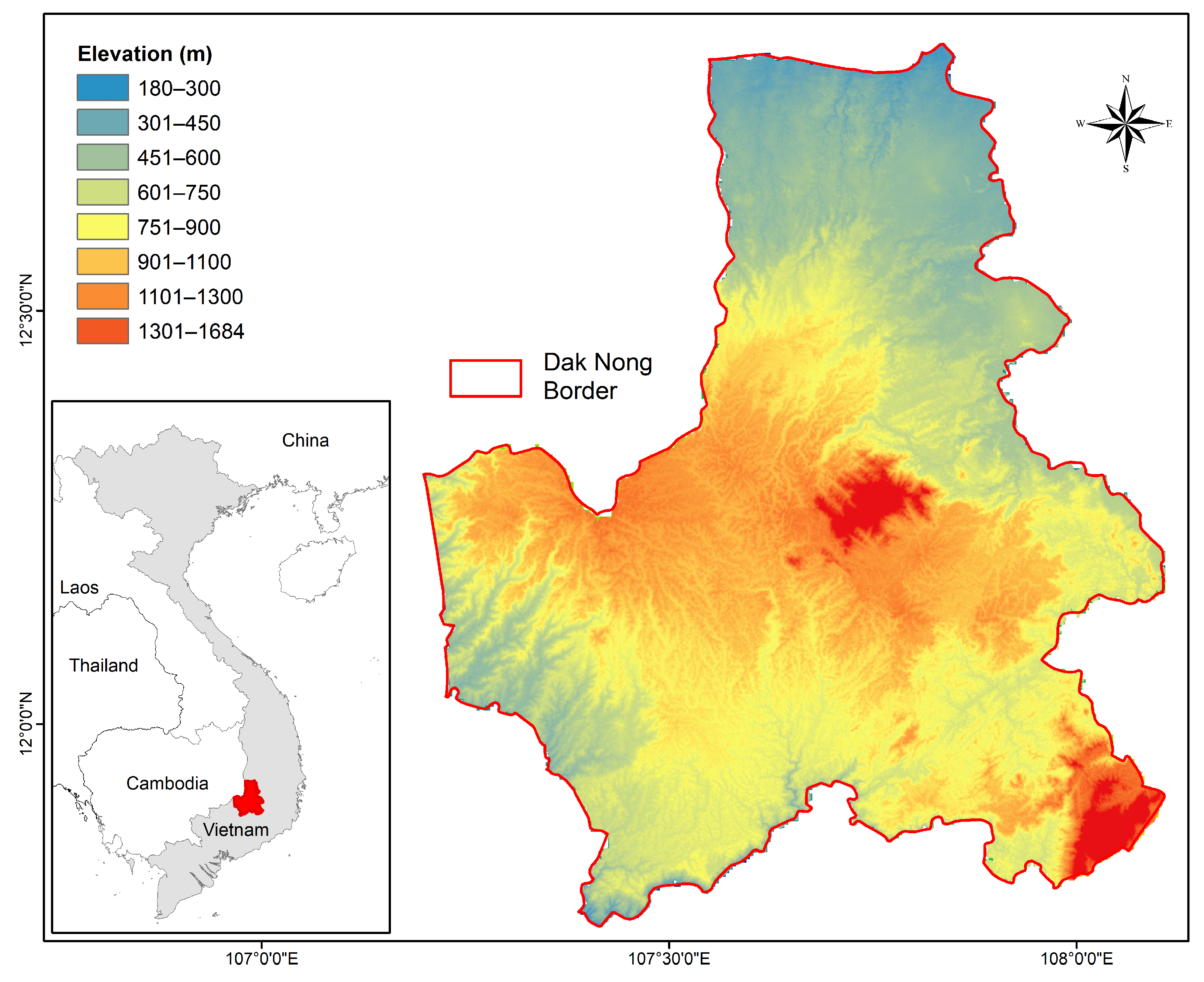
Figure 1. Study area map.
Sustainability 15 05695 g001
Figure 2. The general workflow performed in this study.
Sustainability 15 05695 g002
Figure 3. VHIs’ trend with a p = 0.01 significance level.
Sustainability 15 05695 g003
Figure 4. (a,b) VCI’s and TCI’s trend based on land use types, and (c,d) VCI and TCI based on soil types.
Sustainability 15 05695 g004
Figure 5. The Perennial Agriculture and overlaid with VCI’s trend.
Sustainability 15 05695 g005
Figure 6. The relationship between the VHIs’ trends and the population density.
Sustainability 15 05695 g006
Figure 7. The ratio of the area where the VHIs tend to increase (p) to the part that tends to decrease (1 − p).
Sustainability 15 05695 g007
Figure 8. (a) VHIs’ trend, and (b) Percentage of areas with an increased VHIs’ trend on areas with a clear VHIs’ trend. The white cells are no data.
Sustainability 15 05695 g008
Figure 9. The ratio of the area where the VHIs tends to increase to the area with clear trends correspond to (a) classes in Table 5, and (b) land use types and soil types.
Sustainability 15 05695 g009
Figure 10. Area of (a) land use types and (b) soil types according to the class of population density.
Sustainability 15 05695 g010
Figure 11. The simulation area distribution is not accurate.
Sustainability 15 05695 g011
Figure 12. The accuracy of the discriminant function according to predictor variables. (a) classes in Table 5, (b) land use types and soil types.
Sustainability 15 05695 g012
Table 1. Land use and their description.
Land Use TypeSymbolArea (%)
Perennial AgriculturePeA38.0
Production ForestPdF24.1
Annual CropsAnC14.4
Protection ForestPtF5.6
Special-use ForestSpF5.0
Unused LandUnL1.1
Paddy RicePdR0.7
Table 2. Soil types and their description.
Soil TypeFAO SymbolArea (%)
Rhodic FerralsolsFRr41.7
Plinthic FerralsolsFRp22.0
Xanthic FerralsolsFRx8.3
Haplic ArenosolsACh3.2
Chromic LuvisolsLVx3.2
Arenic AcrisolsACa3.0
Gleyic LuvisolsLVg1.4
Gleyic FluvisolsFLg1.3
Table 3. The coefficients of the logistic regression equation simulate the VHIs’ trend with the independent variables of land use or soil.
 The Independent Variable Is Land UseThe Independent Variable Is Soil
 Land Use TypesVCITCISoil TypesVCITCI
Exp(b)PdF0.070.05ACa0.090.07
UnL0.090.37FRp0.170.14
AnC0.180.76FRx0.510.60
SpF0.930.98 *FRr0.590.61
PeA1.147.88ACh0.720.62
PdR3.7529.63FLg5.285.81
   LVg12.3313.54
b00.528−1.470 0.4630.369
Correct (%)74.175.5 62.164.4
Note: The non-significant case (p > 0.01) in this table is denoted by an asterisk “*”.
Table 4. Characteristic of the land use types and soil with clear VHIs’ trend.
  P_Density (ng/ha)D_Road
(m)
D_River
(m)
Slope
(o)
Land use typesPdF0.3291410752.4
UnL0.224836752.4
AnC0.620085082.2
PeA0.911482401.8
PdR1.86962141.3
Soil typesACa0.720176451.3
FRp0.626258202.4
FLg1.010471521.3
LVx1.67812761.2
LVg1.17681991.3
Table 5. The classes of independent variables for regression model.
P_Density
(People/ha)
P_Rate
(%/year)
Elevation
(m)
Slope
(Degree)
D_Rivers
(m)
D_Roads
(m)
Class
0.1−5.52000.0001
2
3
4
5
6
7
0.30.64000.8250250
0.51.45501.3500500
0.81.96501.810001000
1.22.97502.515001500
1.84.68503.520002500
3.012.09505.025004000
30.014.0120035.0800013,000
Table 6. Standardized coefficients of discriminant function and structure matrix according to a step by step.
  Standardized Canonical Discriminant Function CoefficientsStructure Matrix
  Step 1Setp 2Step 3Step 1Step 2Step 3
VCIP_Density0.5190.5270.5280.7130.7170.718
LU0.5170.5150.5190.6500.6540.654
Soil0.3470.3410.3430.4360.4390.439
P_Rate0.1810.2360.2370.3970.4000.400
D_Roads0.1180.1120.1150.3540.3560.357
D_Rivers0.0170.018 0.3400.342 
Elevation0.128  0.187  
Slope0.018  0.159  
TCIP_Density0.5640.577 0.7000.713 
LU0.4470.445 0.5520.562 
Soil0.2930.295 0.3880.395 
P_Rate0.2180.291 0.3630.369 
D_Roads0.1740.178 0.3560.362 
D_Rivers0.1550.156 0.3530.359 
Elevation0.172  0.193  
Slope0.104  0.182  
Table 7. Canonical discriminant function coefficients and accuracy.
 VCITCI
P_Density2.3772.719
LU2.2202.275
Soil2.0212.029
P_Rate1.8221.969
D_Roads0.7281.161
D_Rivers 1.155
(Constant)−4.026−4.862
Correct (%)82.385.8
Disclaimer/Publisher’s Note: The statements, opinions and data contained in all publications are solely those of the individual author(s) and contributor(s) and not of MDPI and/or the editor(s). MDPI and/or the editor(s) disclaim responsibility for any injury to people or property resulting from any ideas, methods, instructions or products referred to in the content.