Abstract
Investigating the fiscal decentralization’s effect on the carbon intensity of agricultural production may assist the United States in reaching its carbon peak and becoming carbon neutral. This paper delves into the investigation of the spatiotemporal patterns and internal relationships between fiscal decentralization, agricultural carbon intensity, and environmental regulation. The goal was achieved by using the spatial Durbin model using panel data for 49 states of the United States from 2000 to 2019. The study has found that environmental regulations play a significant role in reducing regional carbon emissions in agriculture and contribute positively to carbon emissions control. However, fiscal decentralization, which grants local governments more financial autonomy, has a positive but insignificant impact on carbon emissions, indicating that the prioritization of economic development and carbon control over environmental protection is favored by local governments. In examining the impact of environmental regulations on carbon emissions, the study reveals that fiscal decentralization does not play a substantial role in moderating this relationship. To promote low-carbon agriculture projects and ensure coordinated economic and environmental development, the study recommends optimizing the fiscal decentralization system, formulating different policies for different regions, and regulating the competencies of local governments through an effective examination system. The study concludes that it is crucial to obtain data at the city or county level to accurately understand the relationship between agricultural carbon intensity, environmental regulation, and fiscal decentralization. As a result, the central government must focus on perfecting the fiscal decentralization system, developing a differentiated agricultural carbon emission control system, controlling competition among local governments, and perfecting a political performance assessment system.
1. Introduction
Excessive worldwide emissions of greenhouse gases (primarily CO2) are the primary source of air pollution and the greenhouse effect. They have resulted in climate change and global warming, impacting human life. The United States joined the worldwide movement to decrease carbon dioxide emissions by vigorously campaigning for energy saving and emission reduction [1,2,3]. The United States is still amid industrialization [4]. Its expanding population and rapid urbanization imply that it will be impossible for the economy to wean itself entirely off conventional fossil fuels anytime soon. The goal of the United States is to reach carbon neutrality by 2060 and to reach peak levels of carbon dioxide emissions by the year 2030 while carrying out the global effort to reduce carbon emissions and manage those emissions under the Paris Agreement rather than committing to ‘zero emissions’ like other countries.
After industry, agriculture is the second greatest provider of carbon dioxide [5,6,7]. A lot has to be done to meet the ‘double carbon’ target. Although the United States has far fewer agricultural workers compared to China or India, it still manages to rank third in agricultural production, generating a whopping USD 307.4 billion. Out of this amount, USD 306.4 billion is attributed to food production, which was achieved using only 8.36% of the country’s fertile land (Figure 1) [8,9].
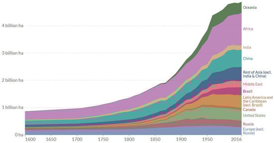
Figure 1.
Agricultural areas over the long term, 1600 to 2016 (OurWorldInData.org/land-use CC BY).
From 1949′s 113.18 million tons, 2020′s projected total grain production of 669.49 million tons is a significant increase. This high food production, however, is backed by the heavy use of fertilizer and pesticides and the reliance on conventional fossil fuels for power. As a result, there is much room for reducing carbon emissions and establishing low-carbon agriculture in the United States.
In a fiscally decentralized system, environmental governance depends on the actions of local governments. Reducing carbon emissions, increasing energy efficiency, and addressing the externalities of pollution are all successes for environmental control [10,11,12,13,14]. While the United States has made great strides in environmental protection, the country’s policies remain starkly divided between urban and rural areas. The United States’ environmental governance system aims to reduce pollution in urban areas and factories. The dichotomy between urban and rural areas falls short in effectively mitigating agricultural pollution, rendering it difficult to prevent and leading to widespread dispersion with indeterminate spatial, temporal, and quantitative patterns [15]. Because of this, the effect of environmental regulations on the amount of carbon dioxide released by agriculture is more readily influenced by the actions of local governments [16,17,18,19]. The question, therefore, becomes, how can fiscal decentralization, environmental control, and carbon emissions in farming all tie together? Would fiscal decentralization affect agricultural carbon emissions less if ecological regulations had a ‘race to the bottom’ quality? We argue that the race to the bottom in environmental law is a crucial factor limiting the potential of fiscal decentralization. To this end, it is essential to investigate fiscal decentralization and environmental control within the same analytical framework. In the same breath, coordinating the connection between agricultural carbon emissions and agricultural economic growth is fundamental to lowering farm emissions. This research thus employs an indicator, agricultural carbon intensity, which may simultaneously represent agricultural economic development and carbon emissions from agriculture. Our study focuses on optimizing the fiscal decentralization system by suggesting coordinated growth of agricultural economics and a reduction in agricultural carbon emissions. The goal is to coordinate the development of the agricultural sector with the effort to reduce carbon emissions from farms and to give policy recommendations as a point of reference for improving the fiscal decentralization system.
Fiscal decentralization, agricultural carbon intensity, and environmental regulation are the essential techniques covered in this research report. The process of moving decision-making authority from a central government to local governments or organizations such as corporations or people is known as fiscal decentralization. Environmental regulation includes laws, regulations, and policies aimed at minimizing pollution by limiting emissions into air, water, and land resources. Agricultural carbon intensity estimates how much CO2 is released per unit of output generated by agricultural activities such as crop production and may be used to analyze China’s agricultural sector’s sustainability performance.
There is currently a lack of research on the effects of fiscal decentralization on agricultural carbon intensity in the United States. There is still debate, and confirmation is needed of how fiscal decentralization impacts environmental regulation. This paper’s authors propose a hypothesis that there is a link between fiscal decentralization and agricultural carbon intensity in the United States. This study makes three significant additions to previous research: it adds an analysis methodology that considers the interplay between fiscal decentralization, agricultural carbon intensity, and environmental regulation. Therefore, this study’s findings are helpful for further clarifying the underlying process of fiscal decentralization, environmental law, and agricultural carbon intensity. There is a lack of literature that examines their connection in the United States. Second, most academics have looked at fiscal decentralization to see how it affects agricultural economic development or to talk about its connection to agricultural carbon emissions, both of which are essential contributions. While many researchers have looked at either the agricultural economy or agricultural carbon emissions, few have looked at both. Third, this research ensures the precision of its estimated findings by using Spatial Durbin Model (SDM) to analyze the connection between fiscal decentralization, agricultural carbon intensity, and environmental regulation.
Another distinguishing feature of this study is that it covers a 20-year period beginning in 2000 and ending in the present, enabling a more nuanced comprehension of the spatial and temporal dynamics underlying the development of agricultural carbon intensity, environmental regulation, and fiscal decentralization in the United States.
The article will then continue as follows: we present Literature Review and Research Hypothesis sections, then we estimate the United States’ agricultural carbon intensity using the above methodologies and data and present the Results and Discussion including the finding from the empirical research. The section titled Conclusions, Policy Implications, and Research Prospects presents an assessment of the limitations of the paper as well as potential avenues for future investigation.
2. Literature Review
This research sheds new light on the relationship between fiscal decentralization (F.D.) and ecological sustainability in the United States. There seems to be a discrepancy in the literature, as far as we can tell. In contrast to [20], we used ecological footprint (E.F.) to measure sustainability rather than environmental performance. Carbon dioxide (CO2) emissions have become a popular metric. Nevertheless, the existing body of literature has been subject to criticism for its inadequate comprehension of the myriad factors that contribute to a sustainable ecosystem. This metric has recently been considered because it excludes the individual’s environmental impact. Therefore, E.F. has become a focal point since it is a more cutting-edge measurement [21,22]. It integrates the paradigms of mitigating the detrimental effects of anthropogenic activities and managing the unsustainable utilization of global natural assets to combat ecological degradation [23]. Qiao et al. [24] study contributes to the field by using modern time-series estimating techniques to investigate the effect of F.D. on E.F. The study’s results also provide improved understanding as well as critical data, outcomes, and evidence of ecological safety, which are useful for policymakers, climate activists, and public representatives.
There has been no comprehensive analysis of how fiscal decentralization in the United States affects agricultural carbon intensity. However, its mechanism research reveals that fiscal decentralization first impacts agricultural economic growth, then agricultural carbon emissions, and last, agricultural carbon intensity. Researchers have shown that fiscal decentralization positively affects agricultural economics [25]. The efficiency with which resources are allocated and the consequent expansion of the economy may both be considerably enhanced by the devolution of fiscal power to regional and municipal governments [26]. Local governments strive to create a conducive business environment and facilitate economic development to enhance the appeal and competitiveness of their respective regional capital markets. This objective stems from the fact that local authorities recognize the direct correlation between economic growth and promotional incentives [27]. Almost all of the public services needed by people living in rural areas of the United States are funded and supplied by the central government. Because of fiscal decentralization, local governments are better equipped to deliver agriculture-friendly public goods and services [28]. Furthermore, agricultural output, financial aid for agriculture, and compulsory schooling in rural areas all benefit from fiscal decentralization [29,30,31].
Several studies have been done on the relationship between agricultural carbon emissions and agricultural economic growth. The consensus among these studies is that the two are tightly linked. Using the Kaya formula and considering the current state of agricultural carbon emissions, [32] concluded that the level of mechanization in agriculture, the structure of agriculture, and the economic development capacity are all crucial factors in reducing emissions. Researchers [33,34] discovered that increases in agricultural added value, increasing the share of the workforce employed in agriculture, and the amount of arable land per person, all leading to lower emissions of greenhouse gases. Additionally, farm carbon emissions are connected with factors such as energy use, fertilizer usage, planted area, and water availability [6,18,35]. It is evident that as the agricultural economy grows, so will agrarian carbon emissions. According to an examination of the relationship between the two mechanisms, environmental regulations affect agricultural carbon emissions primarily through agricultural economics and agricultural carbon emissions. There are three schools of thought about the connection between eco-law and the agriculture sector. In line with the Porter hypothesis, the first perspective agrees with this theory. It maintains that businesses may benefit economically and environmentally from acceptable environmental legislation by engaging in more creative production and waste reduction [36,37]. The second school of thought holds that the Porter hypothesis is not rock solid, and that environmental regulation would slow the expansion of the agriculture sector [38]. According to the third theory, geographical disparities, industry types, and the quality of environmental management all contribute to the ambiguity around how environmental regulations would affect the agricultural sector [39,40,41,42]. The research analysis suggests that the second perspective may be more accurate when describing the effects of environmental legislation on China’s agriculture industry. That is because China is still behind the United States and other high-income Asian nations in agricultural technology innovation and invests far less in agricultural research and development (R&D) than they do [43,44,45]. The influence of environmental rules on the agricultural industry is hampered by the sector’s inherent features, such as a lengthy production cycle, high capital pressure, delayed return, and limited anti-risk capacity. The majority of academics who have studied the relationship between environmental rules and agricultural carbon emissions have concluded that environmental controls may help decrease agricultural carbon emissions. In particular, this is shown in the fact that the objective of lowering agricultural carbon emissions may be attained by the implementation of environmental rules that successfully reduce pollution emissions from farms. According to [46], groundwater in Denmark has greatly improved thanks to stricter environmental rules. Plastic film recycling is positively impacted by environmental legislation, according to [20].
The following paragraphs address the relevant literature and its results concerning fiscal decentralization in the United States. According to [47], the United States Environmental Protection Agency (USEPA) issues permits and sets minimum criteria for ambient air quality and emissions standards (air pollution by factories, power plants, and mobile sources such as vehicles) for each state of the United States. Several states exceed the ambient monitoring standards set by USEPA. However, stronger green-group participant states are more likely to enact air pollution regulations that exceed USEPA criteria [48]. In addition, the race to the top among the states under the Reagan and Bush reforms regime is supported by data obtained by [49,50]. Though governments are granted discretion in making strategic regulatory choices [51], offered very little evidence to indicate the existence of a race to the bottom. It has been argued that decentralization may cause environmental pollution varying from nation to country [52], and it has been argued [53] that political and economic elements are necessary to decide whether there is a race to the top or a race to the bottom.
While there is some evidence that environmental legislation can cut down on carbon emissions from agriculture, the evidence is not conclusive [54,55]. Scholars have conducted a literature review that examines the impact of fiscal decentralization on the carbon intensity of agricultural production and the link between environmental regulation and agricultural carbon intensity. The theoretical model, information, and procedures are covered in the next section. The third part describes the results based on the techniques used. The conclusion and a summary of the potential policy are included in the last paragraph.
2.1. Research Hypothesis
2.1.1. Fiscal Decentralization and Agricultural Carbon Intensity
In the agricultural sector, carbon intensity serves as a crucial measure for balancing economic expansion and greenhouse gas emissions. The formula for determining agricultural carbon intensity reveals that as carbon emissions from farms increase, agricultural carbon intensity rises, and the level of agricultural economic development declines. The influence of fiscal decentralization on agricultural carbon intensity in the United States model continues to be an area of interest. Previous research indicates that fiscal decentralization has a ‘reducing’ impact on the carbon intensity of agriculture [56,57,58]. Furthermore, in accordance with the decoupling theory concerning carbon emissions and the framework regarding agricultural technological progression, a gradual reduction in the influence of agricultural economic growth on carbon emissions within the agricultural sector is envisaged [59,60,61]. Based on these observations, this research proposes the following hypothesis:
H1.
Increased fiscal decentralization is hypothesized to have a negative impact on agricultural carbon intensity.
2.1.2. Agricultural Carbon Intensity and Environmental Regulation
This research suggests that free-riding and mutual imitation could play a role in how environmental regulations affect the United States’ agricultural carbon emissions. The pollution control system of the United States, however, is chiefly oriented towards addressing the issue of industrial and urban pollution. Achieving a reduction in agricultural carbon emissions is proving to be an arduous task due to the primary emphasis of the United States’ pollution control system on industrial and urban pollution, as indicated by [62]. This skewed focus is compounded by the political evaluation framework that prioritizes economic parameters over agricultural carbon emissions. The political assessment mechanism accords greater significance to economic indicators while giving relatively less weight to carbon emissions originating from agricultural activities. Governments will conceal carbon emissions from agriculture to protect economic indices, leading to adverse selection behavior counterproductive to efforts to reduce agricultural carbon emissions [63]. At the same time, free-riding may become the norm since agricultural carbon emissions originate from various ambiguous and non-uniform sources.
In contrast, the impacts of environmental legislation tend to benefit everyone. The ‘I emit, you govern’ mentality of local governments, encouraged by the political rivalry system and the need for rapid economic growth, has resulted in a race to the bottom in environmental legislation to reduce agricultural carbon emissions. The agricultural industry’s growth in the United States has been impeded by the implementation of environmental laws. This slowing may be further undermined by the race to the bottom and free-riding phenomena, which reduce the effectiveness of policies intended to reduce greenhouse gas emissions from agriculture. In light of this, the following theory is advanced in this investigation:
H2.
Even though environmental regulations would reduce the carbon intensity of agriculture, there will be an adverse geographical spillover impact.
2.1.3. Fiscal Decentralization, Agricultural Carbon Intensity, and Environmental Regulation
This study aims to analyze the mechanism of agricultural carbon intensity by combining fiscal decentralization and environmental control within a single framework.
Investigating the agricultural industry and carbon emissions from agriculture that integrates fiscal decentralization and environmental regulation into a single framework is still in its infancy. The vast majority of the extant work examines the impact of environmental restrictions on the agricultural sector or agricultural carbon emissions in the context of United States-style fiscal decentralization. Destruction of the competition in designing and implementing ecological laws [64] impairs fiscal distribution since local governments are motivated by self-interest rather than central government priorities. A phenomenon known as the ‘green paradox’ is set in motion when rights influence the amount of carbon produced by farms [65]. Accordingly, the following theory is advanced in this investigation:
H3.
The ‘green paradox’ effect is caused by fiscal decentralization which, owing to environmental regulation’s race to the bottom features, prevents it from lowering agricultural carbon intensity.
3. Research Methods and Data
3.1. Estimation of Agricultural Carbon Emissions
All forms of agriculture (including horticulture, forestry, animal husbandry, and fisheries) are considered in this investigation. Due to the absence of official statistics, the agricultural carbon emissions of the United States have been estimated in this research, while simultaneously addressing this issue. Although the number and complexity of factors contributing to agricultural carbon emissions are constantly growing, the following four categories have been identified as significant contributors in the past. Farm supplies include raw coal, gas, fuel, power, pesticides, fertilizers, and agricultural film. Second, rice cultivation is a significant source of methane emissions. The third category includes methane and nitrous oxide emissions from livestock production, most notably from the fermentation of animal feces and other waste products in the intestines. Nitrous oxide is a kind that is produced when crops are planted and then released into the atmosphere. One ton of methane has a greenhouse effect equal to 6.8182 tons of C, and one ton of nitrous oxide has a greenhouse impact corresponding to 81.2727 tons of C, as stated in the IPCC’s fifth assessment report on the state of the world’s climate [66]. These equations for agricultural carbon emissions were proposed by [3,67,68], all of which are cited in this work:
where represents agricultural emissions, represents carbon dioxide emissions from the i-th kind of carbon source, C represents agricultural carbon emissions, and —represents the emission coefficient for the i-th type of carbon source. Carbon emission coefficients from prior research [69,70] are used here.
3.2. Measurement of Agricultural Carbon Intensity
Reducing the carbon intensity of agriculture is an efficient means of achieving low-carbon development in the United States agriculture sector. So, the definition of agricultural carbon intensity in this research is based on [3,71]:
where ACI is the dependent variable of agricultural carbon intensity, stands for the agricultural carbon dioxide emissions determined by Equation (1), and A.V. stands for the primary industry produce value-added.
3.3. Variables and Data
3.3.1. Independent Variable: Fiscal Decentralization (F.D.)
While there are several approaches to quantifying fiscal decentralization, the effect of local government budgetary autonomy on agricultural carbon emissions is the main topic that this study covers. The research employed the ratio of per capita fiscal spending as a proxy for the degree of budgetary decentralization, drawing inspiration from [32,72]. In addition, research shows that restructuring government spending due to fiscal decentralization would impact agricultural growth in the area [73,74].
3.3.2. Independent Variable: Environmental Regulation (E.R.)
Collaboration, persuasion, regulation, and economics are the four main types of environmental control [75]. In this analysis, economic regulation is considered an environmental regulation since it is the most efficient means of internalizing external costs. Further, this study aims to represent the environmental protection consciousness and initiatives for the control of the environment within municipal governments’ purview. The available data and practical considerations necessitate the use of the investment-to-GDP ratio as a representation of environmental regulation in the context of environmental pollution control [76,77].
3.3.3. Control Variable
The IPAT and STIRPAT models were used in this investigation to identify applicable control variables. These two models are used to investigate the most critical elements in CO2 output [1,78,79,80]. One standard method of doing so is via the IPAT model, which measures the influence of external factors. Population, wealth, and technological advancement are potential influences on ecosystem health. To account for other possible environmental impacts, the IPAT model was expanded into the STIRPAT model, which allows for the disaggregation of population, wealth, and technology. Therefore, the STIRPAT and IPAT models categorize the control variables: population size, economic status, technological sophistication, and others. The rate of urbanization and rural population density are used as proxies for population variables. Efforts to reduce agricultural carbon emissions may be aided by progressively replacing vast output with intense farming as rural populations grow [6,31]. Rapid urbanization means workers in the countryside will leave for the metropolis. This massive loss of workers might lead to the substitution of fossil fuels for human labor and a subsequent rise in carbon emissions from agriculture [81]. You may use the GDP per capita and the composition of the industrial sector as proxies for economic health. More significant investment in agricultural technology R&D, improved production efficiency, and reduced agricultural carbon intensity may be possible in economically developed and big agricultural provinces [82]. R&D expenditure as a percentage of regional GDP is used to calculate the technical indicators. Technological progress results from increased production efficiency and decreased agricultural carbon emissions [83]. The authors of [84] observed that carbon dioxide emissions are affected by the transportation sector’s influence on energy and environmental efficiency. So, one of the control variables in our analysis is the road traffic infrastructure.
3.3.4. Samples and Data Sources
Forty-nine states of the United States were chosen as representative samples between 2000 and 2019. Various sources included the USDA National Agricultural Statistics Service Information [85], Organization for Economic Cooperation and Development [86], and Statistical Abstract of the United States 2022 [87]. The index was log-transformed to remove heteroscedasticity. The effects of inflation and the price index indicators were revised downward to 2010 levels. Agricultural carbon intensity (ACI), the value-added agricultural carbon dioxide emissions of primary industry, was the dependent variable and was measured as ton/thousand U.S. dollars. The global Moran Index of agricultural carbon intensity is presented in Appendix A Table A1. The independent variables included: (1) fiscal decentralization (F.D.), which is per capita fiscal expenditure; (2) environmental regulation (E.R.), which is the environmental pollution control expenditure percentage of gross domestic product; (3) urbanization rate (U.R.), which is the proportion of percentage of the urban population in the total population; (4) industrial structure, (I.S.) the measure of the percentage of value-added of primary industry to GDP; (5) technique level (T.L.), the percentage of technology research and development expenditure to GDP; (6) road traffic infrastructure (RTI), the total road mileage per unit area measured in kilometers per square kilometer; (7) rural population density (RPD), the total rural population per cultivated area measured as persons per hectare; and (8) per capita gross domestic production (PGDP), measured as gross domestic product divided by the total population.
3.3.5. Estimation of Spatial Autocorrelation of Agricultural Carbon Intensity
Spatial autocorrelation is a phenomenon where observations of certain variables in the same geographical region may exhibit dependency. It measures the extent to which attribute values of geographical units are clustered together. Global spatial autocorrelation provides an overall assessment of this clustering, whereas local spatial autocorrelation examines specific regions where high or low clustering occurs.
3.3.6. Setting of the Spatial Weight Matrix
The selection of an appropriate weight matrix is crucial for the success of any geographic analysis [88]. Contemporary studies typically employ spatial weight matrices such as economic distance, adjacency, and geographic distance matrices. To maintain methodological continuity with prior studies, this investigation employed the methodology put forth by [89,90], which employs the gravity model to create a spatial weight matrix (W1) using the adjacency matrix (W3) and the geographic distance weight matrix (W2). To better represent the rule that the relative importance of economic and geographic elements in variables diminishes continuously with geographical distance, this sort of spatial weight distance matrix considers the underlying economic circumstances of both parties. In a nutshell, the formula is as follows:
where is the spatial weight matrix that was generated using the gravity model; and reflect the average per capita GDP of the state and state from the years 2000 to 2019, respectively; and is the distance that separates state and state from one another. The latitude and longitude coordinates of the two states’ respective capital cities are used to calculate the geographic spherical distance between the two jurisdictions.
3.3.7. Global Spatial Autocorrelation
There may be a geographical relationship between the level of carbon intensity in a region and the level of carbon intensity in agriculture. The global Moran index may take on values between −1 and 1, inclusive. Similar characteristics tend to cluster when the range is between 0 and 1. The strength of space’s positive connection increases as the Moran index approaches 1. When the Moran index is around 1, a high negative correlation exists between the two variables. This range, from 1 to 0, represents various correlations between qualities. The lower the value of the Moran index relative to zero, the less significant the geographical association. The following is the formula for the worldwide Moran index:
The notation I represents the global Moran index, while denotes the total number of observations, represents the spatial weight matrix, and for and j position of the special weight matrix, the and are the observations, respectively, and the average value of is the .
3.3.8. Local Spatial Autocorrelation
This research employed local spatial autocorrelation to investigate the linkage between agricultural carbon intensity and the neighboring states’ agricultural carbon intensity to better examine the geographical variability of agricultural carbon intensity in different states throughout the United States. Here is the formula for the local Moran index:
where is the local Morin index, and all other symbols are as defined in the formula mentioned above (3). State and its neighbors benefit from spatial clustering and have a comparable agricultural carbon intensity if is more than 0. If the value of is nonzero, then the province has a much higher agricultural carbon intensity than neighboring provinces. A Moran scatter plot may be constructed to visualize the regional spatial autocorrelation.
3.3.9. Spatial Econometric Model
Using the information provided in the sections titled “Measurement of agricultural carbon emissions and carbon intensity” and “Variables and data”, the following econometric model was developed. These parts drew on the IPAT and STIRPAT models, respectively:
where represents the intercept term, the coefficient of the variable is denoted by , and represents the random error term. The spatial econometrics theoretical model is an advancement and extension of econometrics that is used to investigate the impact of geographical location on economic activity. Traditional panel regression models typically fail to generate scientific findings in research and analysis because variables have distinct correlations or structures due to different geographic regions. As a result, spatial econometric models need to be implemented to reflect reality better [91]. The spatial lag model (SLM), the spatial error model (SEM), and the SDM are the most often used spatial measurement models. However, in SEM, the spatial lag of the error term is introduced as the independent variable, while in SLM, the spatial lag of the dependent variable is used. The dependent and error variables’ spatial lag term are introduced as independent variables in SDM. The study used the SDM to analyze because the proposed model can capture the spatial impacts of both explanatory and explained variables and the influence of variable error on observation values, which ultimately leads to more accurate conclusions [92].
The study’s SDM formula was as follows:
where denotes the -th state in the United States, where = 1, ⋯, 49; represents the year of observation. The spatial weight matrix is represented by the symbol W. The spatial lag term coefficients for the dependent variable and the independent variable are represented by and , respectively. The random error term for a specific state ith in a given year t is denoted as . The rest of the symbols and variables have the same notation as before.
4. Results and Discussion
4.1. Results for Spatial Panel Regression
In order to select an appropriate spatial measuring model, several tests need to be conducted. In accordance with the principles proposed by [93], this study utilized Stata 17 software to conduct Lagrange multiplier tests to determine the presence of spatial dependence in linear models. The Lagrange multiplier test includes the L.M. test for error dependence (LM-EER) and the simple L.M. test for a missing spatially lagged dependent variable (LMLAG). Moreover, to check whether non-spatial panel data models ignore the spatial effects of the data, this study employed (Robust LM-LAG and Robust LM-ERR).
Table 1 displays statistical data demonstrating that the LM-LAG, LM-ERR, Robust LM-LAG, and Robust LM-ERR tests all passed the 1% significance test, allowing the spatial Durbin estimation model to be implemented. The Wald test, including Wald spatial autoregressive (SAR) and spatial error model (SEM), was used in the analysis, with (p < 0.01) and likelihood ratio (L.R.) including the likelihood ratio spatial autoregressive model (LR-SAR) and likelihood ratio spatial error model (LR-SEM) test with (p < 0.01) to prove that the spatial Durbin estimation model did not degenerate into the SLM model and the SEM model under the circumstances of the spatial Durbin estimation model. At the same time, the Hausman test indicated that the fixed-effects model was superior to the random-effects model (p < 0.01). This investigation fitted the spatiotemporal double fixed-effect spatial Durbin estimation model, as determined by likelihood ratio fixed individual (LR-IND) with (p < 0.01) and likelihood ratio temporal set (LR-TIME) with (p < 0.01).

Table 1.
L.M. test, Wald test, Hausman test, and L.R. test results.
4.2. Results of Spatial Durbin Estimation
This research relied on the gravity model to pick the spatial weight matrix (W1), the geographic distance weight matrix (W2), and the adjacency matrix (W3) for regression analysis, since these three matrices were shown to be the most stable (Table 2). The predicted coefficients were often comparable in sign, magnitude, and significance across the three weight matrices, demonstrating the robustness of the regression findings.
Table 2.
SDM estimation and test results.
From 2000–2019 (Table 2), fiscal decentralization, environmental regulation, industrial structure, technological level, urbanization rate, road transportation infrastructure, and rural population density negatively affected agricultural carbon intensity. This correlates substantially with fiscal decentralization and environmental regulatory interaction factors. Agricultural carbon intensity is significantly bolstered by concurrently present road transportation infrastructure, environmental regulation, industrial structure, and rural population density in nearby regions. Decentralizing government finances and enforcing environmental standards combine to reduce agricultural carbon intensity in powerful ways. Unfortunately, the marginal impact of the independent variable cannot be inferred from the computed coefficient of SDM because of the spatial lag term. Conversely, the independent variable’s direct influence, indirect effect, and overall effect on agricultural carbon intensity must be disentangled to understand it.
4.3. Direct Effects and Spillover Effects of Influencing Factors
As compared to SDM-W1 (R2 = 0.7839) and SDM-W2 (R2 = 0.7936), SDM-W3 has a better R2 value of 0.7962. As a result, the authors decided to focus on both the primary and secondary consequences of SDM-W3 (Table 3). The direct impact is the result of variables inside the province itself, the indirect effect is the result of causes outside the states, and the overall effect is the sum of the two.
Table 3.
Direct effect, indirect effect, and the total effect of factors affecting agricultural carbon emissions.
Regarding the direct impacts, the coefficient of fiscal decentralization is −1.362 and is significant at the 1% level. The result is consistent with the prior research findings. As a result, the first hypothesis is correct. Moreover, according to the findings, the coefficient of the environmental regulatory coefficient is −1.148, which is consistent with the prior study’s findings and has passed the significance test at the level of 1%. As a result, the first part of hypothesis 2 is correct.
Similarly, the coefficient of interaction terms of environmental regulation and fiscal decentralization is positive and significant at a 1% level. That indicates that fiscal decentralization would diminish environmental regulation’s inhibitive impact on agricultural carbon intensity. So, the third hypothesis is correct. One possible explanation for this phenomenon is that an increased level of fiscal decentralization gives local governments a greater capacity and incentive to participate in the region’s economic growth and environmental governance. That is especially the case when the performance appraisal mechanism emphasizes economic development and ignores the rigid demands of the agricultural environment. In these situations, the local government effect will become apparent. Emphasizing economy and disregarding governance is a self-interested fiscal spending preference that has lessened the negative impact of environmental legislation on agricultural carbon emissions.
The urbanization rate has a significant negative relationship (−0.166, p < 0.01) with agricultural carbon intensity, making it one of the most significant control variables. Urbanization has the potential to reduce carbon intensity in agricultural production, as supported by the correlations between urbanization, economic development, and agricultural science and technology. Improved industrial structure (coefficient −0.157, p < 0.01), as measured by the ratio of primary industries’ value to GDP, is associated with better environmental conditions for agricultural production, increased investment in agricultural technology, and environmental protection. The technical level (coefficient −1.415, p < 0.05) has a more significant effect on agricultural carbon intensity than any other explanatory variable. Science and technology research and development have resulted in significant reductions in agricultural carbon emissions and increased production efficiency, enabling the development of agricultural green production technology. Road transportation infrastructure (coefficient −0.288, p < 0.01) has a statistically significant impact on agricultural carbon intensity, as improved infrastructure can improve farmers’ knowledge of the importance of environmental preservation and enhance communication between rural areas and the world. Rural population density (coefficient −0.054, p < 0.01) is negatively associated with agricultural carbon intensity, as people in rural areas value their property more, use fewer chemical pesticides and fertilizers, and use more mulch, resulting in lower agricultural carbon intensity.
The findings of the study support half of hypothesis 2 with regard to spillover effects. The coefficient of environmental regulations on agricultural carbon intensity of neighboring regions is statistically significant at 0.597 (p < 0.01), while the coefficient of fiscal decentralization on agricultural carbon intensity in surrounding areas is −0.597 (p < 0.1). However, the coefficient of environmental regulation on agricultural carbon intensity is not statistically significant. Moreover, a positive statistically significant association is found between the urbanization rate and the carbon intensity of agriculture in the vicinity. The siphon effect, which causes rural workers in the surrounding area to congregate in cities, become more pronounced as urbanization increased. This can lead to a significant loss of rural workers, which may necessitate the substitution of fossil fuels for human labor, increasing agricultural carbon emissions. The coefficient of industrial structure on the agricultural carbon intensity of neighboring regions is also notably positive for big agricultural provinces due to their apparent advantages in agricultural technology and money. There is a statistically significant positive correlation between the presence of roads and the carbon intensity of nearby farms. More developed road networks provide better agricultural transportation systems, but this might lead to a localized concentration of agricultural resources that is not good for the region’s potential for low-carbon agricultural growth. There is a statistically significant inverse relationship between GDP per capita and the carbon intensity of agriculture in the region. That demonstrates the economic radiation effect, which occurs when economically developed places spread their wealth, technology, and human capital to the surrounding areas.
4.4. Empirical Results at the Regional Level
In order to explore the divergences in how fiscal decentralization and environmental regulations affect agricultural carbon intensity across various regions of the United States, the research samples were divided between major grain-producing and non-main grain-producing regions. This was due to the differences in their resource endowment, natural environment, and agricultural economic growth. According to the findings presented in Table 4, there exists a negative correlation between environmental regulations and agricultural carbon intensity in non-primary grain-producing regions. The local governments in these areas have a more pronounced impact on agricultural carbon intensity than those in major grain-producing regions since the latter focuses primarily on achieving stable and high-yield grain production. As a result, this can lead to an overuse of chemical pesticides and fertilizers, which reduces the effectiveness of environmental regulations in mitigating carbon emissions.
Table 4.
Empirical results at the level of the region.
Furthermore, the study found that fiscal decentralization has a minimal impact on agricultural carbon intensity in major grain-producing regions, but it can significantly reduce it in secondary and tertiary grain-producing areas. This is because the stability of grain production in major grain-producing regions has a more significant influence on the food security of the United States, thereby resulting in fewer constraints on agricultural carbon emissions in these areas. Consequently, agricultural carbon intensity is less affected by environmental regulation and fiscal decentralization in major grain-producing regions than in non-main grain-producing areas.
4.5. Robustness Testing and Endogenous Test
4.5.1. Robustness Testing
This study re-estimated the model presented in a previous publication by incorporating new measurement indicators for the moderating factors. Specifically, the study calculated the comprehensive index of environmental regulation (E.R. (1)) by considering industrial wastewater discharge, industrial discharge, and industrial smoke and dust discharge. The calculation of the index involved three main steps.
The first step involved standardizing the levels of industrial wastewater discharge, industrial discharge, and industrial soot discharge in each province, as per Equation (8):
where represents the emission of pollutant in state and represents the index’s standardized outcome. indicates the lowest value of the -th pollutant’s emission in all provinces, while represents the highest value of the -th pollutant’s emission in all provinces.
To determine the weights of various pollutants, the following equation, Equation (9), was utilized:
In this equation, denotes the mean level of emissions for the -th contaminant across all states and years. By calculating the weights of different pollutants using this formula, we derived a comprehensive index of environmental regulation for province i, as presented in Equation (10).
The robustness testing results are presented in Table 5, confirming the negative and significant coefficient of fiscal decentralization and environmental regulation, as previously observed. However, the interaction term between fiscal decentralization and environmental law shows a positive and significant coefficient. This indicates that local governments can use fiscal decentralization to support environmental regulatory laws and achieve emission reduction goals. The central and local governments should work together and leverage fiscal decentralization to develop effective carbon management strategies [82,93,94].
Table 5.
Robustness test for substitution moderating variables.
The indirect impacts reveal that the coefficient of fiscal decentralization is still negative and significant, in line with the research hypothesis presented in Table 3. However, it is worth noting that the estimated coefficient of environmental law on agricultural carbon intensity is significantly positive, which contrasts with the findings in Table 3. This inconsistency must be taken into account when analyzing the overall impacts. Nonetheless, these results do not invalidate the study’s findings.
4.5.2. Endogenous Test
Table 6’s benchmark regression results are consistent with Table 3’s direct impacts, suggesting that fiscal decentralization and environmental regulation may lessen agricultural carbon intensity. However, endogeneity issues may undermine the reliability of these findings. To mitigate this concern, the study used the two-stage least squares (2SLS) approach and took commercial housing sales in each province as an instrumental variable. Retail housing sales were chosen as the instrumental variable because the real estate industry is a crucial driver of the United States’ national economic development and a significant source of tax revenue for local governments [95]. Therefore, it reflects a region’s level of fiscal decentralization. However, it appears that real estate growth has little direct impact on farming.
Table 6.
2SLS estimation of instrumental variable.
In summary, our findings indicate a substantial link between commercial real estate transactions and fiscal decentralization, while there is no direct correlation with agricultural carbon intensity. These results satisfy the criteria for an instrumental variable. Furthermore, the effects of fiscal decentralization and environmental regulations on agricultural carbon intensity remain consistent in the 2SLS estimate, which utilizes commercial dwelling sales as an instrumental variable. The Kleibergen–Paap rk L.M. statistic yields a p-value below 1%, and the Kleibergen–Paap rk Wald F statistic surpasses the 10% threshold value of the Stock–Yogo weak identification test. Therefore, utilizing commercial housing sales as the instrumental variable is a valid choice.
5. Conclusions, Policy Implications, and Research Prospects
5.1. Conclusions
The study has determined that fiscal decentralization and environmental regulation can effectively reduce agricultural carbon intensity. However, the impact of fiscal decentralization on environmental law may lead to a race to the bottom effect, which hinders the reduction of agricultural carbon intensity. To control agricultural emissions effectively, the central government must optimize its fiscal decentralization system. It is also necessary to develop differentiated policies for various regions and optimize regulations regarding competition among local governments and performance evaluation systems accordingly.
The findings of the research indicate that environmental regulations have significantly reduced regional carbon emissions in agriculture, demonstrating a negative correlation between carbon emissions and environmental regulations. The study also highlights the positive impact of these regulations on controlling carbon emissions. In order to avoid a race to the bottom scenario in carbon emission management, it is essential for local governments to establish emission reduction targets and a carbon control performance system that promotes active participation in implementing environmental regulatory policies.
On the other hand, the study found that fiscal decentralization has a positive impact on carbon emissions in general, but it is not statistically significant. This suggests that local governments in United States prioritize economic development over environmental protection and carbon control, often overlooking long-term goals such as environmental preservation. In addition, their focus on short-term economic objectives may exacerbate carbon emissions in the region.
Despite the importance of environmental regulations in curbing carbon emissions, their connection appears to be minor amid the rapidly growing US economy. Fiscal decentralization, which involves the transfer of financial power from central authorities to local governments, has been found to have no significant impact on this relationship. This is supported by a negative but statistically insignificant coefficient of the interaction term between regional environmental laws and fiscal decentralization. However, the central government has taken measures to address the issue by assigning reduction targets and establishing an evaluation system for local governments. This system connects the enforcement of environmental regulations to confidential performance evaluations, effectively discouraging environmentally harmful behavior by local governments. Local governments have also benefited from fiscal decentralization, gaining increased financial support and enforcement capabilities for carbon management. Although its impact on the link between environmental regulations and carbon emissions may not be significant, fiscal decentralization presents a glimmer of hope for future environmental sustainability.
As we delve into the impact of environmental regulations on carbon emissions, we find that spatial variability is not a significant factor. However, when it comes to fiscal decentralization, the story takes an interesting turn. The interplay between fiscal decentralization and carbon emissions reveals significant disparities across regions. In the eastern region, the estimated coefficients for fiscal decentralization are negative and significant, while in the western region they are positive and significant. The central area, too, has significant coefficients to contribute.
The real twist in the tale, however, is the moderating effect of fiscal decentralization on the relationship between environmental regulations and carbon emissions. This effect is only significant in the western region, throwing light on the stark differences between regions in terms of their response to environmental regulations. It is a testament to the complexity of the issue at hand as we navigate through various factors, we must pay heed to the nuances of different regions to arrive at a comprehensive understanding.
Based on the study results, there were no observable temporal variations in the effects of environmental regulations and fiscal decentralization, or their intersection term, on carbon emissions. Environmental regulations are legal provisions established by government entities to ensure the preservation of natural resources, such as air quality (Figure 2).
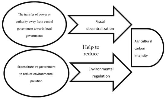
Figure 2.
Relationship between variables.
5.2. Policy Implications
The following policy suggestions are made in light of the findings:
- To boost agricultural economic levels and reduce carbon emissions, the federal government should direct local governments’ fiscal expenditures and prioritize improving the fiscal decentralization system to lean toward low-carbon agriculture projects.
- Based on the state-specific aspects of agricultural development, the central government should upgrade its environmental management authority as appropriate, maintain some degree of centralization in agricultural carbon emission reduction, and replace the traditional environmental regulation mode with a differentiated agricultural carbon emission management system.
- To ensure that economic development is prioritized, and change is optimized, it is imperative for the federal government to regulate the competencies of local governments through an effective examination system. Additionally, this will maximize the effectiveness of the official promotion incentives that are already in place to bring about a shift in the spending patterns of the local government and raise the proportion of carbon emissions in performance evaluation indicators, which will allow for the coordinated economic and environmental development of communities.
5.3. Research Limitations and Prospects
This study focused on examining the complex relationship between fiscal decentralization, environmental regulations, and agricultural carbon intensity in the United States. While acknowledging the potential limitations of our research, we hope that our findings will encourage further investigation into this critical topic. The coefficient values used in our analysis were based on established sources, including official documents from the US government, to maintain the accuracy and validity of our agricultural carbon emission accounting. However, the robustness of the findings is impacted by the continued uncertainty around the coefficients below the state level. The agricultural sector significantly contributes to greenhouse gas emissions and is a potential carbon sink. More precise carbon emissions data may be produced in the future because of improvements in the methods used to compute carbon emissions and carbon absorption. Lastly, obtaining data at the city or county level is necessary, since there are patent differences in agricultural development between regions within a state, to show a more accurate and explanatory relationship between agricultural carbon intensity, environmental regulation, and fiscal decentralization.
Author Contributions
Conceptualization, N.A., K.U.R. and P.S.; Data curation, N.A.K.; Formal analysis, B.H.; Funding acquisition, P.S.; Investigation, Z.H. and A.W.-S.; Methodology, N.A. and B.H.; Project administration, P.S.; Resources, N.A.K.; Software, K.U.R., Z.H., A.W.-S. and P.S.; Supervision, N.A. and P.S.; Validation, N.A., K.U.R., Z.H., N.A.K., A.W.-S., P.S. and B.H.; Visualization, K.U.R. and B.H.; Writing—original draft, N.A., K.U.R. and N.A.K.; Writing—review & editing, Z.H., N.A.K., A.W.-S. and P.S. All authors have read and agreed to the published version of the manuscript.
Funding
This research received no external funding.
Institutional Review Board Statement
Not applicable.
Informed Consent Statement
Not applicable.
Data Availability Statement
Data are openly accessed and freely available to everyone.
Conflicts of Interest
The authors declare no conflict of interest.
Appendix A
Table A1.
Global Moran index of agricultural carbon intensity.
Table A1.
Global Moran index of agricultural carbon intensity.
| Year | Moran Index | Z-Statistics | p-Value | Year | Moran Index | Z-Statistics | p-Value |
|---|---|---|---|---|---|---|---|
| 2000 | 0.088 | 2.100 | 0.010 | 2010 | 0.085 | 1.659 | 0.031 |
| 2001 | 0.089 | 1.987 | 0.014 | 2011 | 0.099 | 1.847 | 0.019 |
| 2002 | 0.093 | 2.098 | 0.010 | 2012 | 0.087 | 1.611 | 0.036 |
| 2003 | 0.089 | 2.153 | 0.008 | 2013 | 0.075 | 1.359 | 0.062 |
| 2004 | 0.095 | 2.036 | 0.012 | 2014 | 0.091 | 1.537 | 0.042 |
| 2005 | 0.092 | 1.850 | 0.019 | 2015 | 0.064 | 1.196 | 0.087 |
| 2006 | 0.114 | 2.138 | 0.009 | 2016 | 0.067 | 1.229 | 0.081 |
| 2007 | 0.099 | 1.939 | 0.016 | 2017 | 0.064 | 1.107 | 0.102 |
| 2008 | 0.098 | 1.849 | 0.019 | 2018 | 0.034 | 0.741 | 0.190 |
| 2009 | 0.108 | 2.139 | 0.009 | 2019 | 0.031 | 0.688 | 0.205 |
References
- Liu, H.; Song, Y. Financial development and carbon emissions in China since the recent world financial crisis: Evidence from a spatial-temporal analysis and a spatial Durbin model. Sci. Total Environ. 2020, 715, 136771. [Google Scholar] [CrossRef]
- Wang, K.; Che, L.; Ma, C.; Wei, Y.-M. The shadow price of CO2 emissions in China’s iron and steel industry. Sci. Total Environ. 2017, 598, 272–281. [Google Scholar] [CrossRef] [PubMed]
- Zhang, L.; Pang, J.; Chen, X.; Lu, Z. Carbon emissions, energy consumption and economic growth: Evidence from the agricultural sector of China’s main grain-producing areas. Sci. Total Environ. 2019, 665, 1017–1025. [Google Scholar] [CrossRef] [PubMed]
- Atack, J.; Margo, R.A.; Rhode, P.W. Industrialization and urbanization in nineteenth century America. Reg. Sci. Urban Econ. 2022, 94, 103678. [Google Scholar] [CrossRef]
- Gul, A.; Chandio, A.A.; Siyal, S.A.; Rehman, A.; Xiumin, W. How climate change is impacting the major yield crops of Pakistan? An exploration from long-and short-run estimation. Environ. Sci. Pollut. Res. 2022, 29, 26660–26674. [Google Scholar] [CrossRef] [PubMed]
- Rehman, A.; Ma, H.; Ahmad, M.; Irfan, M.; Traore, O.; Chandio, A.A. Towards environmental Sustainability: Devolving the influence of carbon dioxide emission to population growth, climate change, Forestry, livestock and crops production in Pakistan. Ecol. Indic. 2021, 125, 107460. [Google Scholar] [CrossRef]
- Rehman, A.; Ma, H.; Ozturk, I. Decoupling the climatic and carbon dioxide emission influence to maize crop production in Pakistan. Air Qual. Atmos. Health 2020, 13, 695–707. [Google Scholar] [CrossRef]
- Food and Agriculture Organization of the United Nations. Statistical Yearbook. 2020. Available online: https://www.fao.org/3/cb1329en/CB1329EN.pdf (accessed on 12 December 2022).
- FRED Economic Data, St. Louis Fed. Employment Level—Agriculture and Related Industries. Economic Research. 2020. Available online: https://fred.stlouisfed.org/series/LNS12034560 (accessed on 12 December 2022).
- Pan, X.; Ai, B.; Li, C.; Pan, X.; Yan, Y. Dynamic relationship among environmental regulation, technological innovation and energy efficiency based on large scale provincial panel data in China. Technol. Forecast. Soc. Chang. 2019, 144, 428–435. [Google Scholar] [CrossRef]
- Zhang, W.; Li, G.; Uddin, M.K.; Guo, S. Environmental regulation, foreign investment behavior, and carbon emissions for 30 provinces in China. J. Clean. Prod. 2020, 248, 119208. [Google Scholar] [CrossRef]
- Zhao, J.; Jiang, Q.; Dong, X.; Dong, K. Would environmental regulation improve the greenhouse gas benefits of natural gas use? A Chinese case study. Energy Econ. 2020, 87, 104712. [Google Scholar] [CrossRef]
- Ahmed, N.; Areche, F.O.; Nieto, D.D.C.; Borda, R.F.C.; Gonzales, B.C.; Senkus, P.; Siemiński, P.; Skrzypek, A. Nexus between Cyclical Innovation in Green Technologies and CO2 Emissions in Nordic Countries: Consent toward Environmental Sustainability. Sustainability 2022, 14, 11768. [Google Scholar] [CrossRef]
- Ahmed, N.; Areche, F.O.; Sheikh, A.A.; Lahiani, A. Green Finance and Green Energy Nexus in ASEAN Countries: A Bootstrap Panel Causality Test. Energies 2022, 15, 5068. [Google Scholar] [CrossRef]
- Merrington, G.; Nfa, L.W.; Parkinson, R.; Redman, M.; Winder, L. Agricultural Pollution: Environmental Problems and Practical Solutions; CRC Press: Boca Raton, FL, USA, 2002. [Google Scholar]
- Madsen, P.M. Does corporate investment drive a “race to the bottom” in environmental protection? A reexamination of the effect of environmental regulation on investment. Acad. Manag. J. 2009, 52, 1297–1318. [Google Scholar] [CrossRef]
- Yijing, C.; Jue, W. The Dilemma and solution of Water pollution Control from the Perspective of Environmental Regulation. E3S Web Conf. 2019, 136, 06007. [Google Scholar] [CrossRef]
- Li, C.; Sun, M.; Xu, X.; Zhang, L.; Guo, J.; Ye, Y. Environmental village regulations matter: Mulch film recycling in rural China. J. Clean. Prod. 2021, 299, 126796. [Google Scholar] [CrossRef]
- Ahmed, N.; Hamid, Z.; Mahboob, F.; Rehman, K.U.; Ali, M.S.e.; Senkus, P.; Wysokińska-Senkus, A.; Siemiński, P.; Skrzypek, A. Causal Linkage among Agricultural Insurance, Air Pollution, and Agricultural Green Total Factor Productivity in United States: Pairwise Granger Causality Approach. Agriculture 2022, 12, 1320. [Google Scholar] [CrossRef]
- Li, W.; Zhang, P. Relationship and integrated development of low-carbon economy, food safety, and agricultural mechanization. Environ. Sci. Pollut. Res. 2021, 28, 68679–68689. [Google Scholar] [CrossRef]
- Alola, A.A.; Bekun, F.V.; Sarkodie, S.A. Dynamic impact of trade policy, economic growth, fertility rate, renewable and non-renewable energy consumption on ecological footprint in Europe. Sci. Total Environ. 2019, 685, 702–709. [Google Scholar] [CrossRef]
- Charfeddine, L. The impact of energy consumption and economic development on ecological footprint and CO2 emissions: Evidence from a Markov switching equilibrium correction model. Energy Econ. 2017, 65, 355–374. [Google Scholar] [CrossRef]
- Qiao, G.; Yang, D.; Ahmad, M.; Ahmed, Z. Modeling for Insights: Does Fiscal Decentralization Impede Ecological Footprint? Int. J. Environ. Res. Public Health 2022, 19, 10146. [Google Scholar] [CrossRef]
- Zahra, S.; Badeeb, R.A. The impact of fiscal decentralization, green energy, and economic policy uncertainty on sustainable environment: A new perspective from ecological footprint in five OECD countries. Environ. Sci. Pollut. Res. 2022, 29, 54698–54717. [Google Scholar] [CrossRef] [PubMed]
- Zhang, X.; Chau, K. An automotive thermoelectric–photovoltaic hybrid energy system using maximum power point tracking. Energy Convers. Manag. 2011, 52, 641–647. [Google Scholar] [CrossRef]
- Lin, J.Y.; Liu, Z. Fiscal decentralization and economic growth in China. Econ. Dev. Cult. Chang. 2000, 49, 1–21. [Google Scholar] [CrossRef]
- Guo, G. China’s local political budget cycles. Am. J. Political Sci. 2009, 53, 621–632. [Google Scholar] [CrossRef]
- Canavire-Bacarreza, G.; Martinez-Vazquez, J.; Yedgenov, B. Identifying and disentangling the impact of fiscal decentralization on economic growth. World Dev. 2020, 127, 104742. [Google Scholar] [CrossRef]
- Ba, Y.M. Democratic Deepening and the Provision of Public Goods: A Study on Decentralization and Agricultural Development in 30 Countries in Sub-Saharan Africa. Ph.D. Thesis, Georgia State University, Atlanta, GA, USA, 2011. [Google Scholar]
- Jain, N.; Sheoran, J. Post economic reforms and Indian agriculture sector: A study of fiscal expenditure and agricultural growth. ZENITH Int. J. Bus. Econ. Manag. Res. 2013, 3, 14–21. [Google Scholar]
- Salqaura, S.; Mulyo, J.; Darwanto, D. The influence of fiscal policy on agriculture sector in Java island. Agro Ekon. 2019, 29, 173–184. [Google Scholar] [CrossRef]
- Ahmed, N.; Mahboob, F.; Hamid, Z.; Sheikh, A.A.; Ali, M.S.e.; Glabiszewski, W.; Wysokińska-Senkus, A.; Senkus, P.; Cyfert, S. Nexus between Nuclear Energy Consumption and Carbon Footprint in Asia Pacific Region: Policy toward Environmental Sustainability. Energies 2022, 15, 6956. [Google Scholar] [CrossRef]
- Chen, X.; Chang, C.-P. Fiscal decentralization, environmental regulation, and pollution: A spatial investigation. Environ. Sci. Pollut. Res. 2020, 27, 31946–31968. [Google Scholar] [CrossRef]
- Cui, H.; Zhao, T.; Shi, H. STIRPAT-Based Driving Factor Decomposition Analysis of Agricultural Carbon Emissions in Hebei, China. Pol. J. Environ. Stud. 2018, 27. [Google Scholar] [CrossRef] [PubMed]
- Cheng, Z.; Li, L.; Liu, J. The spatial correlation and interaction between environmental regulation and foreign direct investment. J. Regul. Econ. 2018, 54, 124–146. [Google Scholar] [CrossRef]
- Cohen, M.A.; Tubb, A. The impact of environmental regulation on firm and country competitiveness: A meta-analysis of the porter hypothesis. J. Assoc. Environ. Resour. Econ. 2018, 5, 371–399. [Google Scholar] [CrossRef]
- Weimin, Z.; Chishti, M.Z.; Rehman, A.; Ahmad, M. A pathway toward future sustainability: Assessing the influence of innovation shocks on CO2 emissions in developing economies. Environ. Dev. Sustain. 2022, 24, 4786–4809. [Google Scholar] [CrossRef]
- Managi, S. Competitiveness and environmental policies for agriculture: Testing the Porter hypothesis. Int. J. Agric. Resour. Gov. Ecol. 2004, 3, 310–324. [Google Scholar] [CrossRef]
- Feix, R.D.; Miranda, S.H.G.d.; Barros, G.S.A.d.C. Environmental regulation and international trade patterns for agro-industrial under a South-North Perspective. In Proceedings of the 2008 International Congress, Ghent, Belgium, 26–29 August 2008. [Google Scholar]
- Kriechel, B.; Ziesemer, T. The environmental Porter hypothesis: Theory, evidence, and a model of timing of adoption. Econ. Innov. New Technol. 2009, 18, 267–294. [Google Scholar] [CrossRef]
- Song, Y.; Wei, Y.; Zhu, J.; Liu, J.; Zhang, M. Environmental regulation and economic growth: A new perspective based on technical level and healthy human capital. J. Clean. Prod. 2021, 318, 128520. [Google Scholar] [CrossRef]
- Tovey, H. Agricultural development and environmental regulation in Ireland. In Agricultural Transformation, Food and Environment; Routledge: Oxfordshire, UK, 2017; pp. 109–130. [Google Scholar]
- Chai, Y.; Pardey, P.G.; Chan-Kang, C.; Huang, J.; Lee, K.; Dong, W. Passing the food and agricultural R&D buck? The United States and China. Food Policy 2019, 86, 101729. [Google Scholar]
- Ahmed, N.; Sheikh, A.A.; Hassan, B.; Khan, S.N.; Borda, R.C.; Huamán, J.M.C.; Senkus, P. The Role of Educating the Labor Force in Sustaining a Green Economy in MINT Countries: Panel Symmetric and Asymmetric Approach. Sustainability 2022, 14, 12067. [Google Scholar] [CrossRef]
- Li, Y.; Zheng, C. Evolution Pattern of Technical Innovation Input and Output of Agricultural Product Processing Industry in China. In Proceedings of the 2018 2nd International Conference on Management, Education and Social Science (ICMESS 2018), Qingdao, China, 23–24 June 2018; pp. 1341–1346. [Google Scholar]
- Hansen, B.; Thorling, L.; Kim, H.; Blicher-Mathiesen, G. Long-term nitrate response in shallow groundwater to agricultural N regulations in Denmark. J. Environ. Manag. 2019, 240, 66–74. [Google Scholar] [CrossRef] [PubMed]
- Potoski, M. Clean air federalism: Do states race to the bottom? Public Adm. Rev. 2001, 61, 335–343. [Google Scholar] [CrossRef]
- Oates, W.E. On the evolution of fiscal federalism: Theory and institutions. Natl. Tax J. 2008, 61, 313–334. [Google Scholar] [CrossRef]
- Fredriksson, P.G.; Svensson, J. Political instability, corruption and policy formation: The case of environmental policy. J. Public Econ. 2003, 87, 1383–1405. [Google Scholar] [CrossRef]
- Millimet, D.L.; List, J.A.; Stengos, T. The environmental Kuznets curve: Real progress or misspecified models? Rev. Econ. Stat. 2003, 85, 1038–1047. [Google Scholar] [CrossRef]
- Konisky, D.M. Regulatory competition and environmental enforcement: Is there a race to the bottom? Am. J. Political Sci. 2007, 51, 853–872. [Google Scholar] [CrossRef]
- Sigman, H. Decentralization and environmental quality: An international analysis of water pollution levels and variation. Land Econ. 2014, 90, 114–130. [Google Scholar] [CrossRef]
- Kim, J.H. Linking land use planning and regulation to economic development: A literature review. J. Plan. Lit. 2011, 26, 35–47. [Google Scholar]
- Li, T.; Liu, Y.; Lin, S.; Liu, Y.; Xie, Y. Soil pollution management in China: A brief introduction. Sustainability 2019, 11, 556. [Google Scholar] [CrossRef]
- Yoder, L. Compelling collective action: Does a shared pollution cap incentivize farmer cooperation to restore water quality? Int. J. Commons 2019, 13, 378–399. [Google Scholar] [CrossRef]
- Zhang, K.; Zhang, Z.-Y.; Liang, Q.-M. An empirical analysis of the green paradox in China: From the perspective of fiscal decentralization. Energy Policy 2017, 103, 203–211. [Google Scholar] [CrossRef]
- He, Q.; Deng, X.; Li, C.; Yan, Z.; Kong, F.; Qi, Y. The green paradox puzzle: Fiscal decentralisation, environmental regulation, and agricultural carbon intensity in China. Environ. Sci. Pollut. Res. 2022, 29, 78009–78028. [Google Scholar] [CrossRef]
- Yang, Y.; Tian, Y.; Peng, X.; Yin, M.; Wang, W.; Yang, H. Research on Environmental Governance, Local Government Competition, and Agricultural Carbon Emissions under the Goal of Carbon Peak. Agriculture 2022, 12, 1703. [Google Scholar] [CrossRef]
- Huang, Q.; Zhang, Y. Decoupling and decomposition analysis of agricultural carbon emissions: Evidence from Heilongjiang province, China. Int. J. Environ. Res. Public Health 2022, 19, 198. [Google Scholar] [CrossRef] [PubMed]
- Liu, W.; Xu, R.; Deng, Y.; Lu, W.; Zhou, B.; Zhao, M. Dynamic relationships, regional differences, and driving mechanisms between economic development and carbon emissions from the farming industry: Empirical evidence from rural China. Int. J. Environ. Res. Public Health 2021, 18, 2257. [Google Scholar] [CrossRef] [PubMed]
- Zhou, M.; Hu, B. Decoupling of carbon emissions from agricultural land utilisation from economic growth in China. Agric. Econ. 2020, 66, 510–518. [Google Scholar] [CrossRef]
- Zhang, W.; Wu, S.; Ji, H.; Kolbe, H. Estimation of China’s agricultural non-point source pollution situation and control countermeasures I. Estimation of China’s agricultural non-point source pollution situation in the early 21st century. China Agric. Sci. 2004, 1008–1017. [Google Scholar]
- Yuan, P.; Zhu, L. Agricultural pollution prevention and control in China: Deficiencies of environmental regulation and the stake holder’s adverse selection. Issues Agric. Econ. 2015, 36, 73–80. [Google Scholar]
- Woods, N.D. The State of State Environmental Policy Research: A Thirty-Year Progress Report. Rev. Policy Res. 2021, 38, 347–369. [Google Scholar] [CrossRef]
- Sinn, H.-W. Public policies against global warming: A supply side approach. Int. Tax Public Financ. 2008, 15, 360–394. [Google Scholar] [CrossRef]
- Pachauri, R.; Meyer, L. Climate Change 2014: Synthesis Report. Contribution of Working Groups I, II and III to the Fifth Assessment Report of the Intergovernmental Panel on Climate Change; IPCC: Geneva, Switzerland, 2014. [Google Scholar]
- Huang, X.; Xu, X.; Wang, Q.; Zhang, L.; Gao, X.; Chen, L. Assessment of agricultural carbon emissions and their spatiotemporal changes in China, 1997–2016. Int. J. Environ. Res. Public Health 2019, 16, 3105. [Google Scholar] [CrossRef] [PubMed]
- Tian, P.; Li, D.; Lu, H.; Feng, S.; Nie, Q. Trends, distribution, and impact factors of carbon footprints of main grains production in China. J. Clean. Prod. 2021, 278, 123347. [Google Scholar] [CrossRef]
- Luo, Y.; Long, X.; Wu, C.; Zhang, J. Decoupling CO2 emissions from economic growth in agricultural sector across 30 Chinese provinces from 1997 to 2014. J. Clean. Prod. 2017, 159, 220–228. [Google Scholar] [CrossRef]
- Zhu, H.; Duan, L.; Guo, Y.; Yu, K. The effects of FDI, economic growth and energy consumption on carbon emissions in ASEAN-5: Evidence from panel quantile regression. Econ. Model. 2016, 58, 237–248. [Google Scholar] [CrossRef]
- Zhou, B.; Zhang, C.; Song, H.; Wang, Q. How does emission trading reduce China’s carbon intensity? An exploration using a decomposition and difference-in-differences approach. Sci. Total Environ. 2019, 676, 514–523. [Google Scholar] [CrossRef]
- Jin, J.; Zou, H.-f. Fiscal decentralization, revenue and expenditure assignments, and growth in China. J. Asian Econ. 2005, 16, 1047–1064. [Google Scholar] [CrossRef]
- Gudeta, T.; Alam, M.; Tolassa, D. The Practices and Challenges of Fiscal Decentralization: A Case of Bedelle Woreda, Oromia Region, Ethiopia. PanAfrican J. Gov. Dev. (PJGD) 2021, 2, 50–80. [Google Scholar] [CrossRef]
- Hong, D.P.T.; Viet, H.N. Fiscal Decentralization and Agricultural Field: Empirical Evidence from Vietnam. J. Appl. Sci. 2016, 16, 462–469. [Google Scholar] [CrossRef]
- Böcher, M. A theoretical framework for explaining the choice of instruments in environmental policy. For. Policy Econ. 2012, 16, 14–22. [Google Scholar] [CrossRef]
- Wang, B.; Wu, Y.; Yan, P. Environmental Efficiency and Environmental Total Factor Productivity Growth in China’s Regional Economies (Zhongguo Quyu Huanjing Xiaolu yu Huanjing Quanyaosu Shengchanlu Zengzhang). Econ. Res. J. 2010, 45, 95–109. [Google Scholar]
- Zhang, M.; Liu, X.; Ding, Y.; Wang, W. How does environmental regulation affect haze pollution governance?—An empirical test based on Chinese provincial panel data. Sci. Total Environ. 2019, 695, 133905. [Google Scholar] [CrossRef]
- Wen, L.; Li, Z. Driving forces of national and regional CO2 emissions in China combined IPAT-E and PLS-SEM model. Sci. Total Environ. 2019, 690, 237–247. [Google Scholar] [CrossRef]
- Zheng, X.; Lu, Y.; Yuan, J.; Baninla, Y.; Zhang, S.; Stenseth, N.C.; Hessen, D.O.; Tian, H.; Obersteiner, M.; Chen, D. Drivers of change in China’s energy-related CO2 emissions. Proc. Natl. Acad. Sci. USA 2020, 117, 29–36. [Google Scholar] [CrossRef]
- Ahmed, N.; Sheikh, A.A.; Mahboob, F.; Ali, M.S.e.; Jasińska, E.; Jasiński, M.; Leonowicz, Z.; Burgio, A. Energy Diversification: A Friend or Foe to Economic Growth in Nordic Countries? A Novel Energy Diversification Approach. Energies 2022, 15, 5422. [Google Scholar] [CrossRef]
- Zhang, N.; Yu, K.; Chen, Z. How does urbanization affect carbon dioxide emissions? A cross-country panel data analysis. Energy Policy 2017, 107, 678–687. [Google Scholar] [CrossRef]
- Yang, H.; Wang, X.; Bin, P. Agriculture carbon-emission reduction and changing factors behind agricultural eco-efficiency growth in China. J. Clean. Prod. 2022, 334, 130193. [Google Scholar] [CrossRef]
- Ismael, M.; Srouji, F.; Boutabba, M.A. Agricultural technologies and carbon emissions: Evidence from Jordanian economy. Environ. Sci. Pollut. Res. 2018, 25, 10867–10877. [Google Scholar] [CrossRef] [PubMed]
- Lin, B.; Chen, Y. Will land transport infrastructure affect the energy and carbon dioxide emissions performance of China’s manufacturing industry? Appl. Energy 2020, 260, 114266. [Google Scholar] [CrossRef]
- USDA, United States Department of Agriculture. National Agricultural Statistics Service Information. 2022. Available online: https://www.nass.usda.gov/Data_and_Statistics/ (accessed on 12 December 2022).
- OECD. Gross domestic product (GDP) (indicator). 2022. Available online: https://www.oecd-ilibrary.org/economics/gross-domestic-product-gdp/indicator/english_dc2f7aec-en (accessed on 12 December 2022).
- Tench, R. Proquest Statistical Abstract of the United States 2022: The National Data Book; Reed Business Information: New York City, NY, USA, 2022. [Google Scholar]
- Feng, Y.; Wang, X.; Du, W.; Wu, H.; Wang, J. Effects of environmental regulation and FDI on urban innovation in China: A spatial Durbin econometric analysis. J. Clean. Prod. 2019, 235, 210–224. [Google Scholar] [CrossRef]
- Earnest, A.; Morgan, G.; Mengersen, K.; Ryan, L.; Summerhayes, R.; Beard, J. Evaluating the effect of neighbourhood weight matrices on smoothing properties of Conditional Autoregressive (CAR) models. Int. J. Health Geogr. 2007, 6, 54. [Google Scholar] [CrossRef]
- Liu, Y.; Dong, F. How industrial transfer processes impact on haze pollution in China: An analysis from the perspective of spatial effects. Int. J. Environ. Res. Public Health 2019, 16, 423. [Google Scholar] [CrossRef]
- Anselin, L. Spatial Econometrics: Methods and Models; Springer: Berlin/Heidelberg, Germany, 1988; Volume 4. [Google Scholar]
- Zhao, P.; Zeng, L.; Li, P.; Lu, H.; Hu, H.; Li, C.; Zheng, M.; Li, H.; Yu, Z.; Yuan, D. China’s transportation sector carbon dioxide emissions efficiency and its influencing factors based on the EBM DEA model with undesirable outputs and spatial Durbin model. Energy 2022, 238, 121934. [Google Scholar] [CrossRef]
- Elhorst, J.P. Specification and estimation of spatial panel data models. Int. Reg. Sci. Rev. 2003, 26, 244–268. [Google Scholar] [CrossRef]
- Chen, Y.; Li, M. The Measurement and Influencing Factors of Agricultural Carbon Emissions in China’s Western Taiwan Straits Economic Zone. Nat. Environ. Pollut. Technol. 2020, 19, 587–601. [Google Scholar] [CrossRef]
- Chong, J.; Phillips, G.M. COVID-19 losses to the real estate market: An equity analysis. Financ. Res. Lett. 2022, 45, 102131. [Google Scholar] [CrossRef]
Disclaimer/Publisher’s Note: The statements, opinions and data contained in all publications are solely those of the individual author(s) and contributor(s) and not of MDPI and/or the editor(s). MDPI and/or the editor(s) disclaim responsibility for any injury to people or property resulting from any ideas, methods, instructions or products referred to in the content. |
© 2023 by the authors. Licensee MDPI, Basel, Switzerland. This article is an open access article distributed under the terms and conditions of the Creative Commons Attribution (CC BY) license (https://creativecommons.org/licenses/by/4.0/).