
Toughness Properties of a 50-Year-Old Pipeline Material


Abstract
1. Introduction
2. Materials and Methods
- -
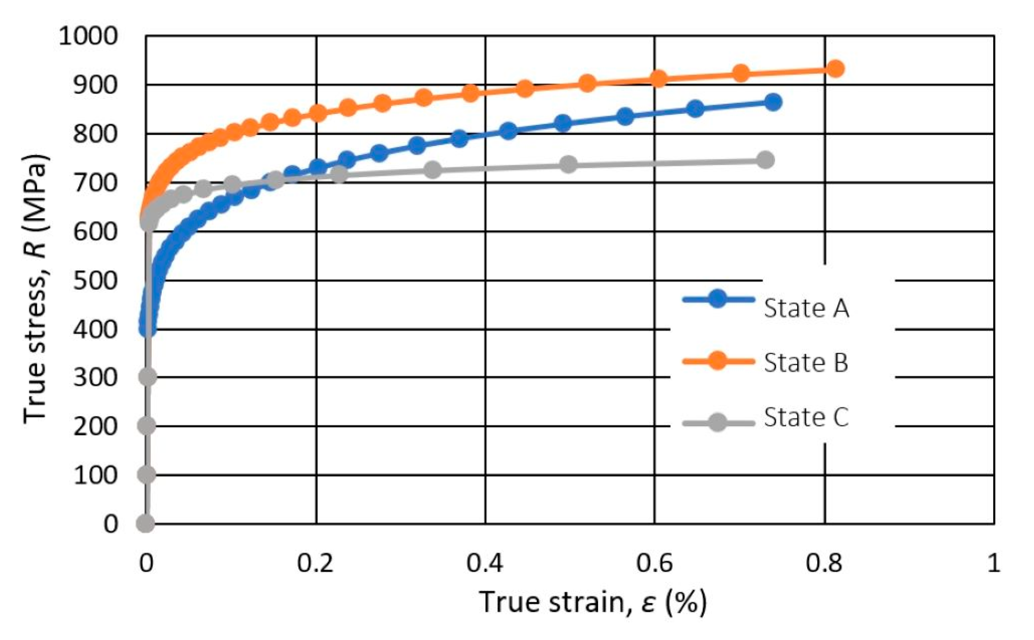
- State A: The normalised state of the material before its deformation and pipe making (undeformed sheets).
- -
- State B: The aged and deformed state, which implies 10% cold deformation and heated for 30 min at +250 °C.
- -
- State C: The deformed state of the material which is in the range of 10% cold deformation.
3. Results Analysis and Discussion
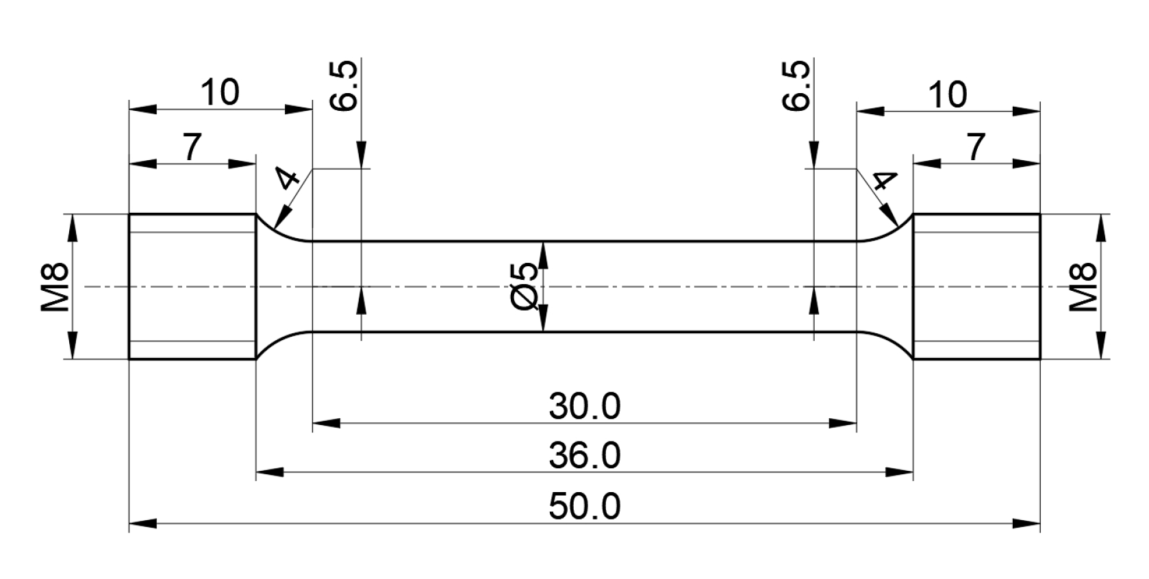
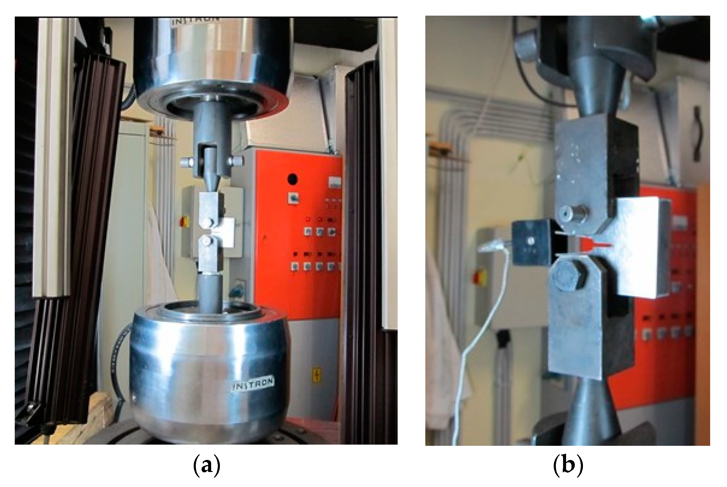
3.1. Tensile Testing
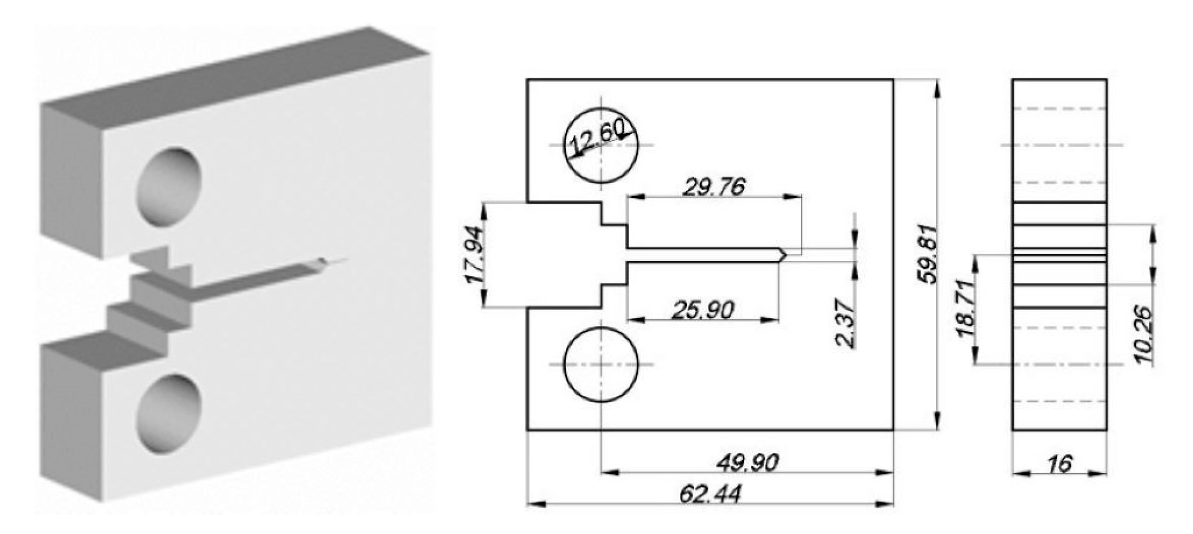
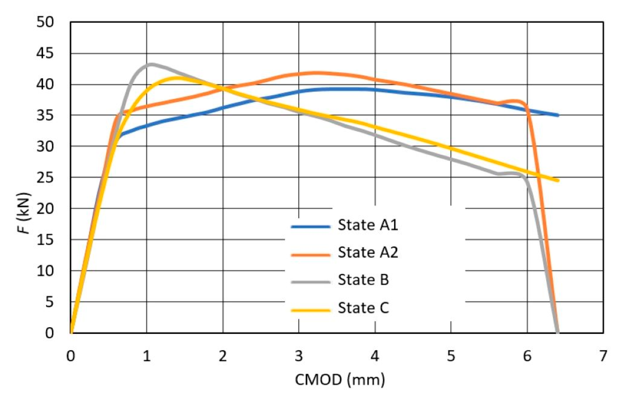
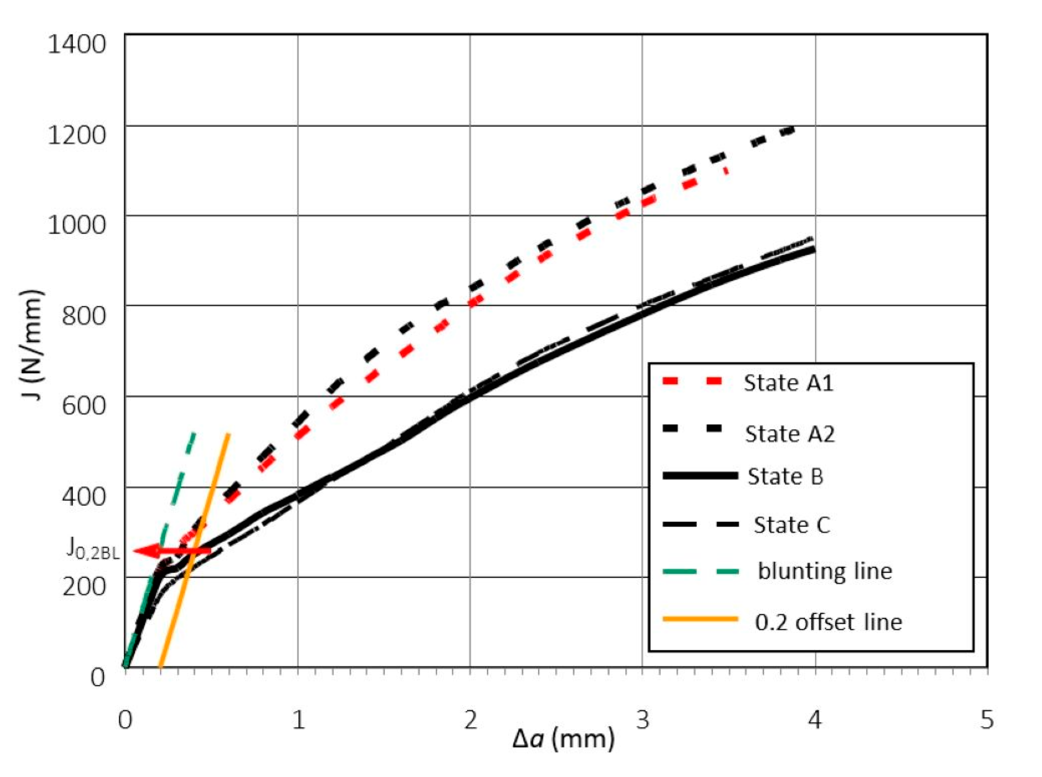
3.2. Examination of Fracture Mechanics
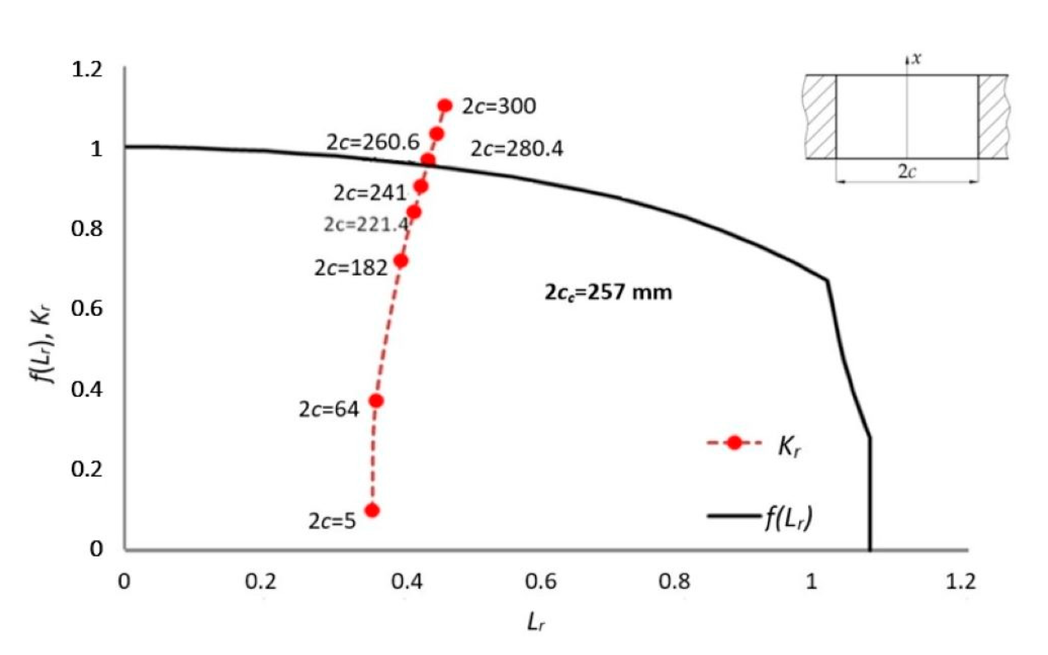
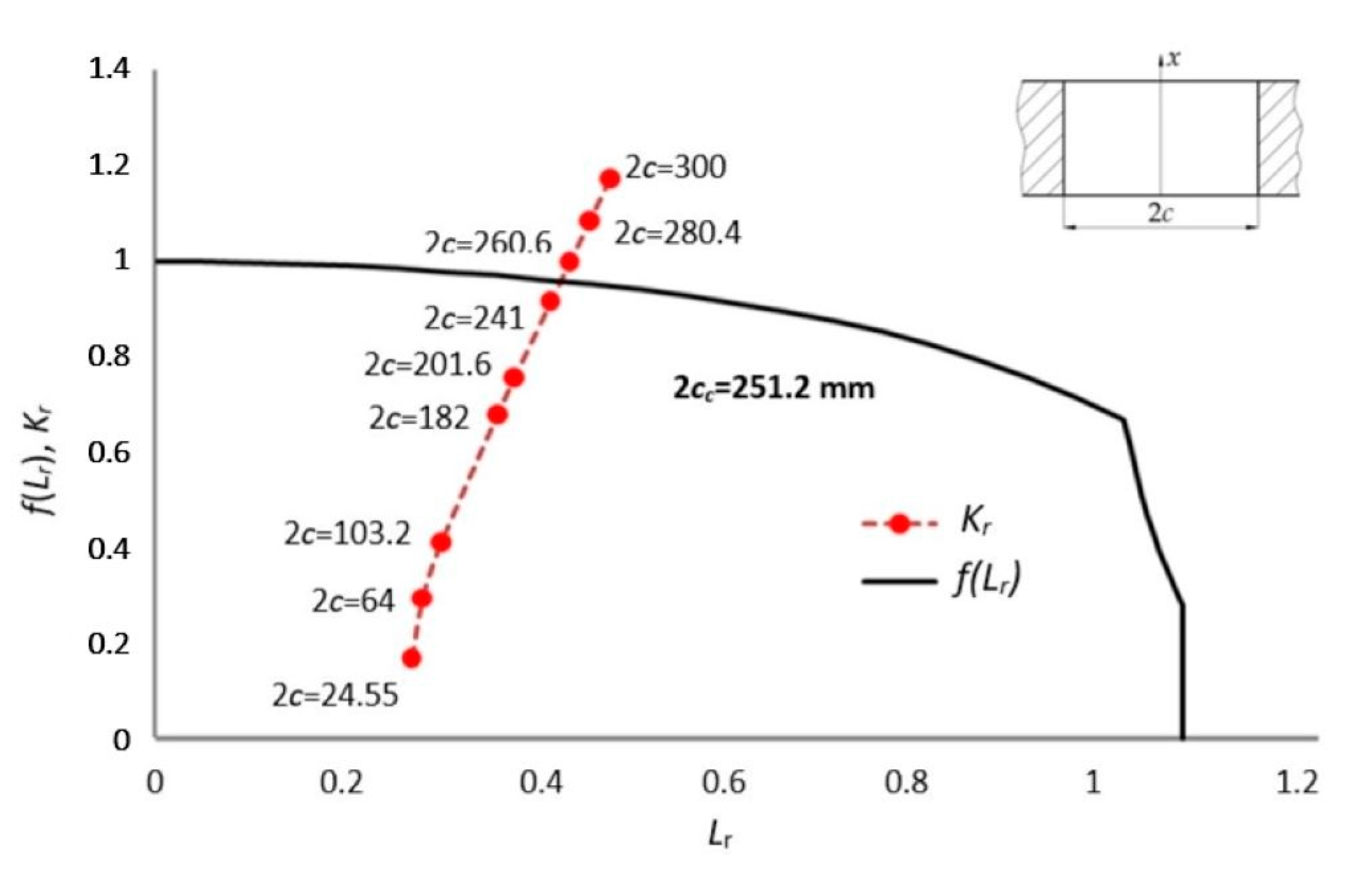
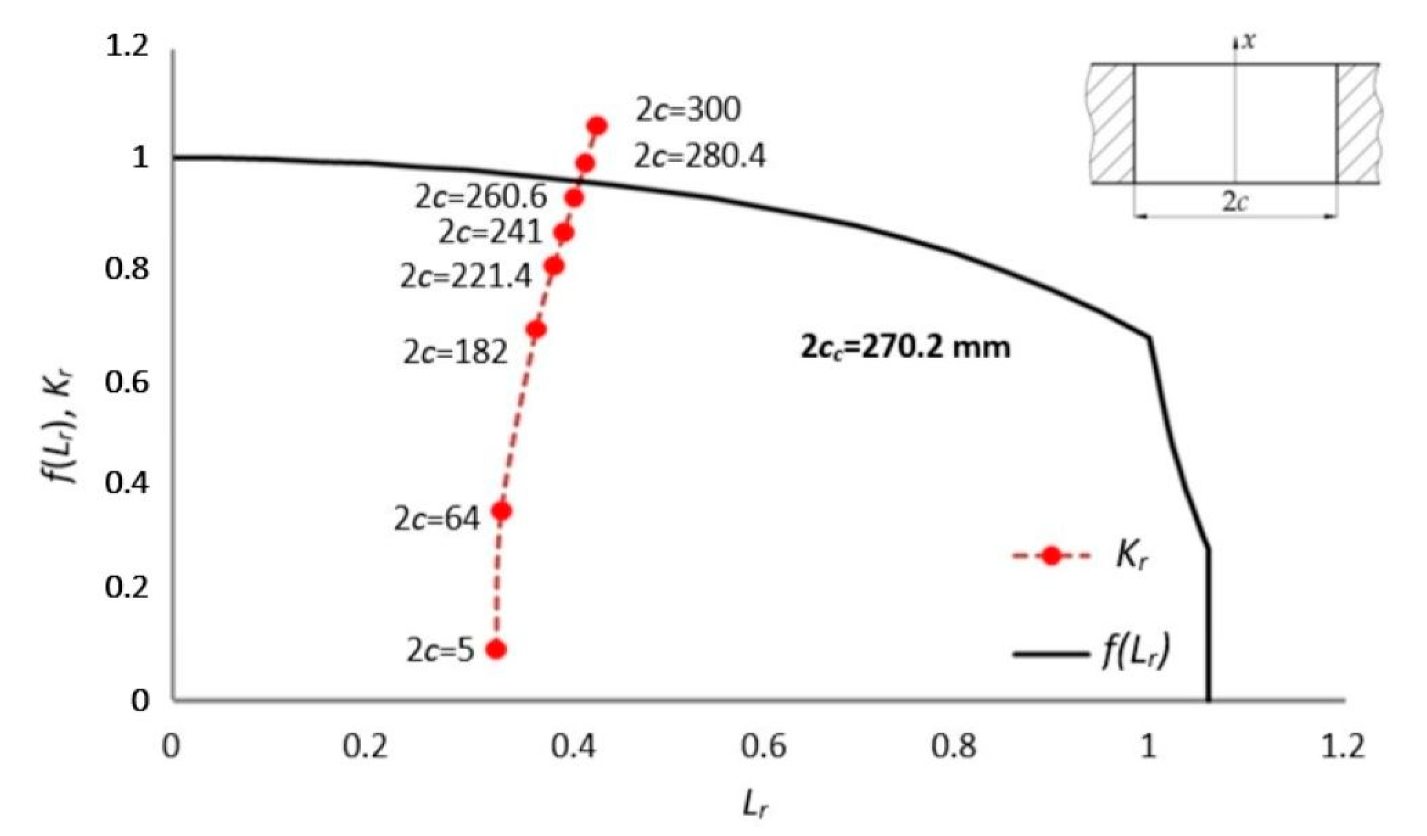
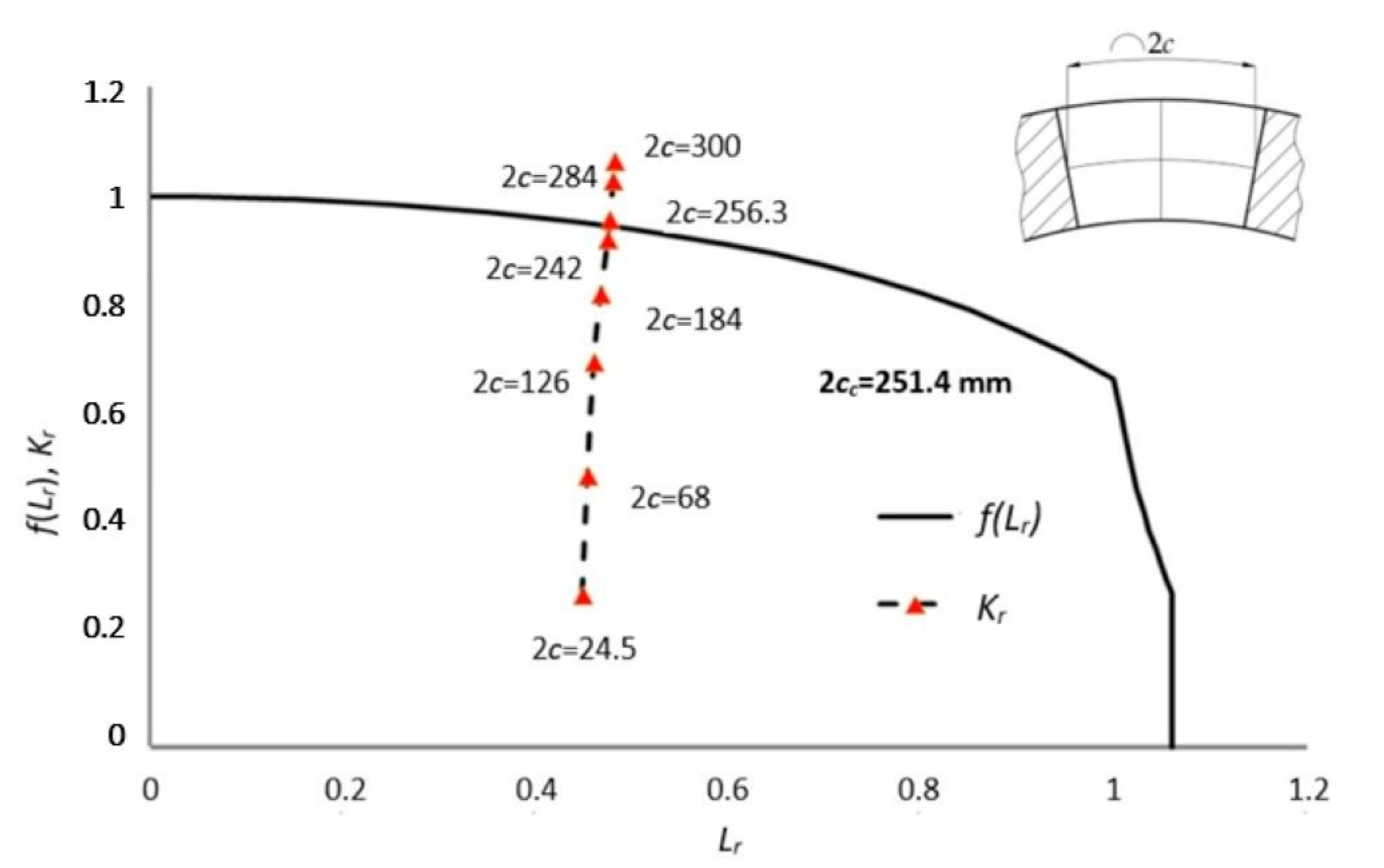
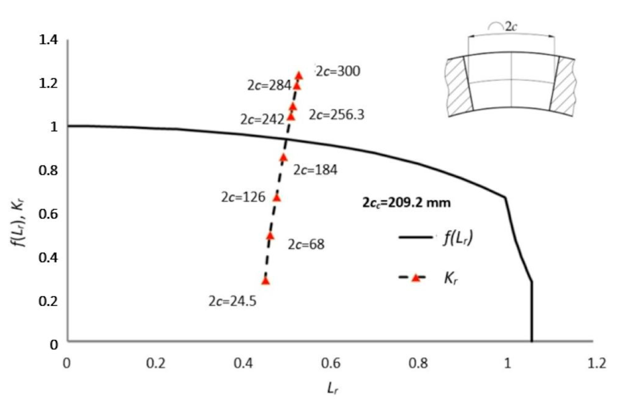
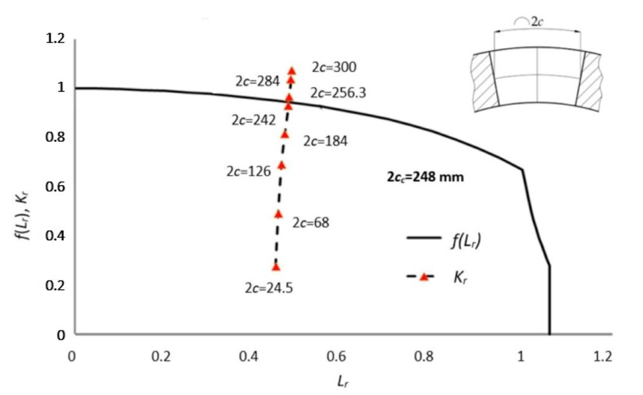
3.3. Calculation of Critical Crack Length
SINTAP Procedure, Level “1”
- -
- -
- ETM, which was developed by HZG (Helmholtz-Zentrum Hereon) [32].
4. Conclusions
Funding
Institutional Review Board Statement
Informed Consent Statement
Data Availability Statement
Acknowledgments
Conflicts of Interest
References
- Sang, Z.F.; Xue, L.P.; Lin, Y.J.; Widera, G.E.O. Limit and burst pressures for a cylindrical shell intersection with inter-mediate diameter ratio. Int. J. Press. Vessel. Pip. 2002, 79, 341–349. [Google Scholar] [CrossRef]
- Ćulafić, S.; Maneski, T.; Bajić, D. Stress Analysis of a Pipeline as a Hydropower Plant Structural Element. J. Eng. Mech. 2020, 66, 51–60. [Google Scholar] [CrossRef]
- Barry, R.M.; Venter, G. Analysis of reinforcement designs for specials in steel pipelines. Int. J. Press. Vessel. Pip. 2019, 169, 204–214. [Google Scholar] [CrossRef]
- Skopinsky, V.N. Numerical stress analysis of intersecting cylindrical shells. J. Press. Vessel Technol. 1993, 115, 275–282. [Google Scholar] [CrossRef]
- Sedmak, S.; Sedmak, A. Integrity of Penstock of Hydroelectric Powerplant. Struct. Integr. Life 2005, 5, 59–70. [Google Scholar]
- Qiuping, M.; Guiyun, T.; Yanli, Z.; Rui, L.; Huadong, S.; Zhen, W.; Bin, G.; Kun, Z. Pipeline In-Line Inspection Method, In-strumentation and Data Management. Sensors 2021, 21, 3862. [Google Scholar] [CrossRef]
- Sachedina, K.; Mohany, A. A review of pipeline monitoring and periodic inspection methods. Pipeline Sci. Technol. 2018, 2, 187–201. [Google Scholar] [CrossRef]
- Arsić, M.; Malešević, Z.; Mladenović, M.; Savić, Z.; Bošković, G. Analysis of Current State and Integrity Evaluation of the Pipeline at Hydro Power Plant. In IMK-14—Research & Development in Heavy Machinery; University of Kragujevac: Kragujevac, Serbia, 2017; Volume 23, pp. 9–14. [Google Scholar]
- El Fakkoussi, S.; Moustabchir, H.; Elkhalfi, A.; Pruncu, C. Computation of the stress intensity factor KI for external longitudinal semi-elliptic cracks in the pipelines by FEM and XFEM methods. Int. J. Interact. Des. Manuf. 2019, 13, 545–555. [Google Scholar] [CrossRef]
- Moustabchir, H.; Hamdi Alaoui, M.A.; Babaoui, A.; Dearn, K.D.; Pruncu, C.I.; Azari, Z. The influence of variations of geometrical parameters on the notching stress intensity factors of cylindrical shells. J. Theor. Appl. Mech. 2017, 55, 559–569. [Google Scholar] [CrossRef]
- Zareei, A.; Nabavi, S.M. Calculation of stress intensity factors for circumferential semi-elliptical cracks with high aspect ratio in pipes. Int. J. Press. Vessel. Pip. 2016, 146, 32–38. [Google Scholar] [CrossRef]
- Li, C.Q.; Fu, G.; Yang, W. Stress intensity factors for inclined external surface cracks in pressurised pipes. Eng. Fract. Mech. 2016, 165, 72–86. [Google Scholar] [CrossRef]
- ASTM E1820-18; Standard Test Method for Measurement of Fracture Toughness. American Society for Testing and Materials: West Conshohocken, PA, USA, 2018. [CrossRef]
- Faleskog, J.; Barsoum, I. Tension–torsion fracture experiments—Part I: Experiments and a procedure to evaluate the equivalent plastic strain. Int. J. Solids Struct. 2013, 50, 4241–4257. [Google Scholar] [CrossRef]
- Chan, K.S.; Lankford, J. The role of microstructural dissimilitude in fatigue and fracture of small cracks. Acta Metall. 1988, 36, 193–206. [Google Scholar] [CrossRef]
- Smaili, F.; Lojen, G.; Vuherer, T. Fatigue crack initiation and propagation of different heat affected zones in the presence of a microdefect. Int. J. Fatigue 2019, 128, 105191. [Google Scholar] [CrossRef]
- Boyer, H.E. Atlas of Fatigue Curves; ASM International: Metals Park, OH, USA, 1986. [Google Scholar]
- Gao, H.; Wu, Y.F.; Li, C.Q. Performance of normalization method for steel with different strain hardening levels and effective yield strengths. Eng. Fract. Mech. 2019, 218, 106594. [Google Scholar] [CrossRef]
- Chen, X.; Nanstad, R.; Sokolov, M.A.; Manneschmidt, E.T. Determining Ductile Fracture Toughness in Metals. Adv. Mater. Process. 2014, 172, 19–23. [Google Scholar]
- Gao, H.; Wang, W.; Wang, Y.; Zhang, B.; Li, C.Q. A modified normalization method for determining fracture toughness of steel. Fatigue Fract. Eng. Mater. Struct. 2020, 43, 1–16. [Google Scholar] [CrossRef]
- ASTM E1820-05a; Standard Test Method for Measurement of Fracture Toughness. American Society for Testing and Materials: West Conshohocken, PA, USA, 2017.
- SINTAP Structural Integrity Assessment Procedures for Europen Industry; Sub-Task 3.3 Report: Final Issue. Determination of Structure Toughness from Charpy Impact Enegy: Procedure and Validation. Brite-Euram Project No. BE95-1426; British Steel: London, UK, 1998.
- Stephen, W.; Bannister, A. Structural integrity procedure for Europe SINTAP-an overview. Mater. High Temp. 2002, 19, 91–97. [Google Scholar] [CrossRef]
- Brkić, A.; Maneski, T.; Spasojević-Brkić., V.; Golubović, T. Industrial safety improvement of crane cabins. Struct. Integr. Life 2015, 15, 95–102. [Google Scholar]
- Report No. 0306-42/09 on the Examination of the Elliptical Connecting Plate of the Branch Junction 6A (A Side) on the Supply Pipeline No.3 HPP “Perućica”; Black Metallurgy Institute AD: Nikšić, Montenegro, September 2009.
- Report No. 0200000-06/10 on Testing Anchors on Supply Pipelines No.1 and No.3 HPP “Perućica”; Black Metallurgy Institute AD: Nikšić, Montenegro, October 2009.
- Report on Magnetic Particle Tests No.274/01-MT/09—Examination of the Part of the Branch Junction in the Reinforcement Zone from the Inside on the Supply Pipeline No. 3 HPP “Perućica” Nikšić; Center for Control and Testing d.o.o.: Belgrade, Serbia, August 2009.
- Report on Magnetic Particle Tests No.351/01-UT/11—Examination the Homogeneity of the Base Material of the Anchor in the Scope of 100% (Pipeline No.3) HPP “Perućica” Nikšić; Center for Control and Testing d.o.o.: Belgrade, Serbia, January 2011.
- Elaborate on Testing the Stress-Strain State of the Branch Junction A6 on Pipeline C3 HPP “Perućica” Nikšić; Faculty of Mechanical Engineering: Podgorica, Montenegro, 2007.
- Assessment of the Integrity of Structures Containing Defects. Amendment 3; R6 Revision 4; BEGL Procedure; British Energy: Gloucester, UK, 2004.
- Sahu, M.K.; Chattopadhyay, J.; Dutta, B.K. Application of R6 failure assessment method to obtain fracture toughness. Theor. Appl. Fract. Mech. 2016, 81, 67–75. [Google Scholar] [CrossRef]
- Landes, J.D.; Schwalbe, K.H.; Dietzel, W. ETM Format for Creep Deformation Parameters; GKSS-Forschungszentrum Geesthacht GmbH: Geesthacht, Germany, 2004. [Google Scholar]
- Hadley, I. 3-Fracture Assessment Methods for Welded Structures. In Fracture and Fatigue of Welded Joints and Structures; Woodhead Publishing Limited TWI: Cambridge, UK, 2011; pp. 60–90. [Google Scholar]
- Brlić, T. Appearance of Lüders Bands in Niobium Microalloyed Steel. Doctoral Thesis, University of Zagreb, Faculty of Metallurgy, Zagreb, Croatia, 2020. [Google Scholar]
- Shengwen, T.; Xiaobo, R.; Jianying, H.; Zhiliang, Z. Effect of the Lüders plateau on ductile fracture with MBL model. Eur. J. Mech. A Solids 2019, 78, 103840. [Google Scholar] [CrossRef]
- Chapuilot, S. KI Formula for Pipes with a Semi-Elliptical Longitudinal or Circumferential, Internal or External Cracks; CEA Report CEA-R-5900; International Atomic Energy Agency (IAEA): Vienna, Austria, 2000. [Google Scholar]
- Sattari-Far, I.; Dillström, P. Local limit load solutions for surface cracks in plates and cylinders using finite element analysis. Int. J. Press. Vessel. Pip. 2004, 81, 57–66. [Google Scholar] [CrossRef]
- Zang, W. Stress Intensity Factor Solutions for Axial and Circumferential Through-Wall Cracks in Cylinders; Report SINTAP/SAQ/02; SAQ Control AB: Stockholm, Sweden, 1997. [Google Scholar]
- Kiefner, J.F.; Maxey, W.A.; Eiber, R.J.; Duffy, A.R. Failure Stress Levels of Flaws in Pressurized Cylinders; STP49657S; American Society for Testing Material: West Conshohocken, PA, USA, 1973; pp. 461–481. [Google Scholar]
- Al Laham, S. Stress Intensity Factor and Limit Load Handbook; SINTAP/Task 2.6; Report EPD/GEN/REP/0316/98, Issue 2; British Energy Generation Ltd.: Barnwood, UK, 1998. [Google Scholar]


| Material | E, GPa | Rp0.2, MPa | Rm, MPa | Em, % | Ef, % | σ0, MPa | N |
|---|---|---|---|---|---|---|---|
| State A | 196 | 442 | 610 | 13.7 | 27 | 27 | 27 |
| State B | 193 | 647 | 726 | 4.7 | 12 | 12 | 12 |
| State C | 192 | 627 | 684 | 4.5 | 11 | 11 | 11 |
| Parameter | Label | A1 | A2 | B | C |
|---|---|---|---|---|---|
| Initial crack length | a0, mm | 25.052 | 28.089 | 27.797 | 29.766 |
| The ratio of the length of the crack to the width of the compact tension specimen | a0/W | 0.561 | 0.562 | 0.556 | 0.595 |
| Stable increase in crack length | Δastab, mm | 3.495 | 4.020 | 4.412 | 4.525 |
| Crack opening 0.2BL * | J0.2,BL, N/mm | 298 | 305 | 250 | 219 |
| Crack length increment at 0.2BL | Δa0.2BL, mm | 0.570 | 0.540 | 0.307 | 0.336 |
| Maximum force | Fmax, kN | 39.1 | 41.9 | 42.9 | 41.2 |
| Value at Fmax | Jm, N/mm | 635 | 740 | 340 | 315 |
| Fracture toughness of material PSS ** | KI,mat, MPa∙m0.5 | 242 | 244 | 220 | 206 |
| Fracture toughness of material PSN ** | KI,mat, MPa∙m0.5 | 253 | 256 | 230 | 216 |
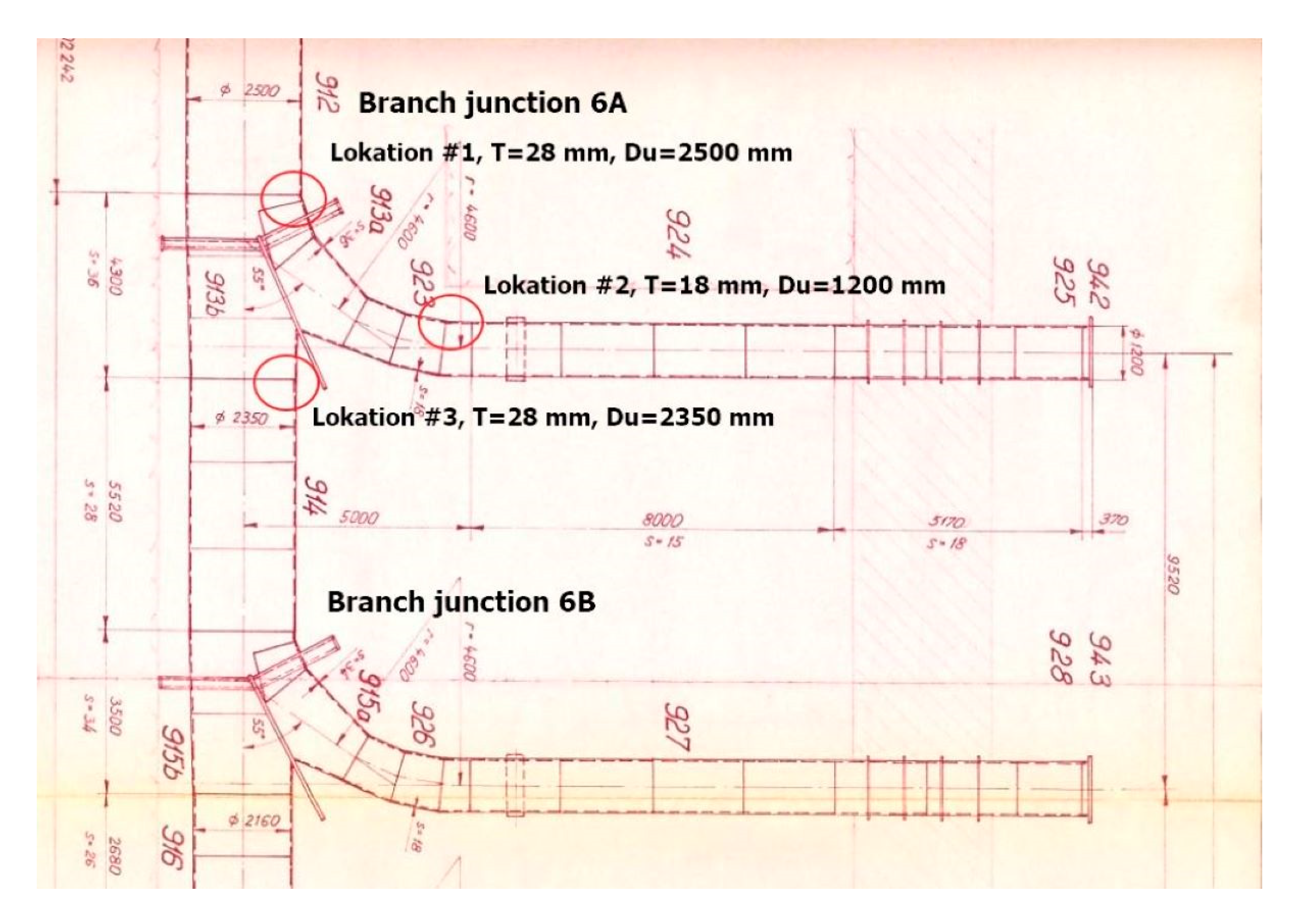
| Location | T, mm | Du, mm | a/c | σ, MPa | ac, mm | 2cc, mm | Comment |
|---|---|---|---|---|---|---|---|
| #1 | 28.0 | 2500 | 0.1 | 227.2 | 25.05 | 500.1 | Fracture before highlighting |
| #2 | 18.0 | 1200 | 0.1 | 169.7 | 17.0 * | 340.0 * | The condition for LBB |
| #3 | 28.0 | 2350 | 0.1 | 213.2 | 26.08 | 521.6 | Fracture before highlighting |
| Location | T, mm | Du, mm | a/c | σ, MPa | a, mm | 2c, mm | Comment |
|---|---|---|---|---|---|---|---|
| #1 | 28.0 | 2500 | 0.2 | 227.2 | 27.0 * | 270.0 * | The condition for LBB |
| #2 | 18.0 | 1200 | 0.2 | 169.7 | 17.0 * | 170.0 * | |
| #3 | 28.0 | 2350 | 0.2 | 213.2 | 27.0 * | 270.0 * |
| Location | T, mm | Du, mm | σ, MPa | 2cc, mm | Comment |
|---|---|---|---|---|---|
| #1 | 28.0 | 2500 | 227.2 | 257.0 * | The condition for LBB |
| #2 | 18.0 | 1200 | 169.7 | 251.2 * | |
| #3 | 28.0 | 2350 | 213.2 | 270.2 * |
| Location | T, mm | Du, mm | σ, MPa | 2c, mm | Comment |
|---|---|---|---|---|---|
| 1 | 28.0 | 2350 | 106.8 | 248.0 | They are fulfilled conditions for LBB |
| 2 | 28.0 | 2500 | 113.6 | 251.4 | |
| 3 | 18.0 | 1200 | 84.8 | 209.2 |
Disclaimer/Publisher’s Note: The statements, opinions and data contained in all publications are solely those of the individual author(s) and contributor(s) and not of MDPI and/or the editor(s). MDPI and/or the editor(s) disclaim responsibility for any injury to people or property resulting from any ideas, methods, instructions or products referred to in the content. |
© 2023 by the author. Licensee MDPI, Basel, Switzerland. This article is an open access article distributed under the terms and conditions of the Creative Commons Attribution (CC BY) license (https://creativecommons.org/licenses/by/4.0/).
Share and Cite
Bajić, D. Toughness Properties of a 50-Year-Old Pipeline Material. Sustainability 2023, 15, 5143. https://doi.org/10.3390/su15065143
Bajić D. Toughness Properties of a 50-Year-Old Pipeline Material. Sustainability. 2023; 15(6):5143. https://doi.org/10.3390/su15065143
Chicago/Turabian StyleBajić, Darko. 2023. "Toughness Properties of a 50-Year-Old Pipeline Material" Sustainability 15, no. 6: 5143. https://doi.org/10.3390/su15065143
APA StyleBajić, D. (2023). Toughness Properties of a 50-Year-Old Pipeline Material. Sustainability, 15(6), 5143. https://doi.org/10.3390/su15065143