Integrating Unsupervised Machine Intelligence and Anomaly Detection for Spatio-Temporal Dynamic Mapping Using Remote Sensing Image Series

Abstract

The synergistic use of remote sensing and unsupervised machine learning has emerged as a potential tool for addressing a variety of environmental monitoring applications, such as detecting disaster-affected areas and deforestation. This paper proposes a new machine-intelligent approach to detecting and characterizing spatio-temporal changes on the Earth’s surface by using remote sensing data and unsupervised learning. Our framework was designed to be fully automatic by integrating unsupervised anomaly detection models, remote sensing image series, and open data extracted from the Google Earth Engine platform. The methodology was evaluated by taking both simulated and real-world environmental data acquired from several imaging sensors, including Landsat-8 OLI, Sentinel-2 MSI, and Terra MODIS. The experimental results were measured with the kappa and F1-score metrics, and they indicated an assertiveness level of 0.85 for the change detection task, demonstrating the accuracy and robustness of the proposed approach when addressing distinct environmental monitoring applications, including the detection of disaster-affected areas and deforestation mapping.

1. Introduction

Preservation is crucial for the maintenance of human life on the planet, as the environment is constantly changing due to anthropogenic actions [1]. Among the biggest global environmental challenges, we can cite the emission of greenhouse gases, massive deforestation, and other critical disturbing disasters that have been catalyzed by the unbridled consumption of natural resources [2]. Concerned with the world environmental scenario, the “United Nations 2030 Agenda” brings a transversal, multidimensional, and holistic vision of this issue; the sustainable development goals dictate how to make human wellbeing, economic prosperity, and environmental protection coexist by supporting public policies for mitigating and coping with the impacts on the environment [3].

Considering the environmental context, Brazil has been at the center of debates, especially because of the Amazon forest, which is the largest tropical forest in the world. Indeed, this biome plays an essential role in maintaining global climate dynamics and regulation [4], as it has undergone intensive deforestation since 2010, thus resulting in landscape disturbances [5]. Additionally, the El Niño–Southern Oscillation (ENSO) events have raised the concentration of ${\mathrm{CO}}_2$ in the atmosphere, increasing the planet’s surface temperature and the burning occurrences in the Amazon forest [6]. La Niña is another genuine example of a phenomenon that leads to landscape disturbance, as it promotes high precipitation and evapotranspiration in the Amazon basin [7], thus causing regional flooding disasters. Finally, there are also landscape disturbances that are caused by catastrophic failures, such as the one that occurred in Brazil because of the collapses of mining dams in the towns of Mariana [8] and Brumadinho [9].

In order to successfully deal with events of environmental change such as those mentioned above, the development of new tools for the constant observation of biomes and humanmade structures is critically important; this includes the creation of new remote-sensing-based technologies. In addition to capturing reflected radiation at different spectral wavelengths, remote sensing has enabled the spatio-temporal tracking of large areas [10,11], which can be computationally performed by using different strategies, such as spectral indices [12]. Another powerful and well-established tool in this context is machine learning, as it allows the design of new algorithms for extracting information and knowledge from large databases [13]. For example, Holloway et al. [14] demonstrated several applications of machine learning methods, which included classification, clustering, and regression models, for the creation of new approaches to achieving the United Nations Sustainable Development Goals.

Anomaly detection (AD) comprises a category of unsupervised machine learning that aims at identifying elements that do not follow an expected behavior [15]. Several studies in the scientific literature have been supported by anomaly detection methods, which include recent applications in domains such as health sciences [16], social monitoring [17], and psychology [18]. Furthermore, anomaly detection methods also appear in the context of remote sensing, e.g., to detect temporal changes on the Earth’s surface [19,20,21].

In contrast to conventional image classification techniques, anomaly detection methods can simultaneously deal with seasonal and atmospheric interferences that may impact the targets’ behavior when distinguishing changes in the Earth’s surface, such as those caused by deforestation [22], technological disasters [23], and wildfires [21]. However, due to limitations imposed by the spatial resolution of remote sensing data [24,25] and considering that anomalies comprise a small portion of the data, algorithms purely based on anomaly detection tend to overestimate the false positive errors [26]. Since seasonal trends and the target’s spectral variability are relevant features that must be preserved when applying anomaly detection methods on remote sensing image series, the use of more sophisticated approaches involving machine learning tasks can improve the discrimination of transient data in time series, thus producing data-driven models that are capable of overcoming these issues.

In light of the above-presented discussions, this paper proposes a new framework that combines anomaly detection models and remote sensing image series, which are expressed in terms of spectral indices, to identify and characterize regions with high spectral–temporal dynamics. Our approach uses the Google Earth Engine (GEE) platform to collect fresh data, allowing the training of data-driven models to discriminate among the transient features of time series of remotely sensed images. Beyond integrating the GEE platform and AD-based methods, the proposed methodology is designed for the mapping of areas with recurrent temporal changes (i.e., highly dynamic areas) in a fully unsupervised way. To the best of the authors’ knowledge, there is no similar proposal that takes as input a time series of remote sensing images and, following an entirely unsupervised process, delivers decision rules for identifying anomalies in remote sensing scenes extracted from a sensor that has been selected. Moreover, in contrast to other methods in the general literature that make use of anomaly detection to identify specific targets or produce susceptibility maps for very particular events, our approach focuses on the good fitting capabilities of unsupervised AD-based models that are adapted to the context of remote sensing for the characterization and identification of recurrent changes of an arbitrary nature. As a result, our framework is flexible enough to be applied in the context of the monitoring of anthropogenic actions, including deforestation and agriculture applications, as well as the analysis of landscape changes caused by disaster events, such as dam failures.

Experiments with simulated data and case studies with actual remote sensing images of regions affected by intense deforestation, as well as technological disasters, were carried out in order to demonstrate the effectiveness and robustness of the proposed methodology.

This paper is organized as follows: Section 2 presents the basic notations, anomaly detection models, and spectral indices; Section 3 proposes our framework for mapping spatio-temporal disturbances; Section 4 covers an extensive set of experiments that used synthetic and actual remote sensing data, and discussions are found in Section 5. Finally, Section 6 concludes our research.

Finally, the aim and hypothesis of this study are given as follows:

• Aim: “Developing an accurate and flexible machine-learning-based method that detects and maps spatio-temporal dynamics by assuming only a time series of remotely sensed images as input.”
• Hypothesis: “Regions subject to frequent disturbances are mapped as anomalies in remote sensing image series.”

2. Theoretical Background

2.1. Preliminary Notations

Let $\mathcal{I}$ be a matrix representing a remotely sensed image. Each pixel/position of $\mathcal{I}$ is expressed by s, which is defined over a regular grid $\mathcal{S}\subset {\mathbb{N}}^2$. The radiance reflected by the Earth’s surface and recorded by the remote sensor is usually expressed by a vector $\mathbf{x}$, which is characterized as an element of the attribute space $\mathcal{X}$. Therefore, $\mathcal{I}\left(s\right)=\mathbf{x}$ represents the behavior of $\mathcal{I}$ with respect to position s, which is given by the d-dimensional vector $\mathbf{x}=[x_1,x_2,\dots ,x_d]$.

Among the different applications supported by remote sensing images, distinguishing targets on the Earth’s surface through machine learning techniques for classification is a typical approach. A classification process stands for applying a function $F:\mathcal{X}\to \mathcal{Y}$ on the attribute vector $\mathbf{x}$ of each $s\in \mathcal{S}$ so as to associate a class $y\in \mathcal{Y}=\left\{1,\dots ,c\right\}$.

The different classification techniques proposed in the literature comprise specific ways of modeling F. Moreover, the learning paradigm dictates the approach to obtaining F. Supervised and unsupervised methods are the usual strategies for learning from data, and they are used for classification purposes [27,28,29,30]. Supervised methods perform the modeling by gathering and analyzing labeled data that are available in a training set $\mathcal{D}=\left\{({\mathbf{x}}_i,y_i)\in \mathcal{X}\times \mathcal{Y}:i=1,\dots ,m\right\}$. On the other hand, unsupervised methods are not supported by training ground-truth sets to model F. Consequently, such methods are not able to define a label (with semantic meaning) for the input data. In this case, the learning process relies on analogies that are found when the dataset is explored. As a result, clusters of similar elements are determined without a particular semantic meaning.

An anomaly detection process comprises a particular case of unsupervised classification, which splits the data into “regular” and “anomalous” elements [31].

2.2. Anomaly Detection

Among a variety of techniques that permeate the machine learning field, anomaly detection methods consist of a useful approach to identifying elements with significantly distinct behavior compared to other observations. In a broad context, anomalies and outliers share similar characteristics, as they stand for elements that present a distinct behavior in comparison to other pixel clusters and segments in an image [23,32,33].

Anomaly detection techniques have been effectively applied to detect bank frauds and intruders in security systems, as well as to support medical analysis [34]. Beyond these applications, anomaly detection methods are also known as a potential tool for environmental monitoring [35,36]. The Local Outlier Factor [37], Elliptic Envelope [38], One-Class Support Vector Machine (OC-SVM) [39], and Isolation Forest (IF) [40] are representatives of anomaly detection methods that are commonly found in the scientific literature. In particular, the OC-SVM and IF methods have been successfully employed in remote sensing studies [21,41,42].

As a variant of the Support Vector Machine (SVM) method, the OC-SVM provides a model for distinguishing the “regular objects” of a set $\mathcal{Z}$ with probability $\nu$ of false-positive occurrence. Formally, the OC-SVM comprises a function $F:\mathcal{X}\to \left\{+1,-1\right\}$ that returns $+1$ when the input data belong to $\mathcal{Z}$, or $-1$ otherwise. This function is given by:

$$F\left(\mathbf{x}\right)=\mathrm{sgn}\left(\sum _{i=1}^n{\alpha }_{i}K(\mathbf{x},{\mathbf{x}}_i)-b\right)$$

(1)

where $b={\sum }_{j=1}^n{\alpha }_{j}K({\mathbf{x}}_i,{\mathbf{x}}_j)$, ${\mathbf{x}}_i\in \mathcal{Z}$, and $K(·,·)$ stands for a kernel function. The coefficients ${\alpha }_i$, $i=1,\dots ,n$, are obtained by solving the following optimization problem:

$$\begin{array}{c}\underset{{\alpha }_1,\dots ,{\alpha }_n}{min}\sum _{i,j=1}^n{\alpha }_i{\alpha }_{j}K({\mathbf{x}}_i,{\mathbf{x}}_j)\hfill \\ s.t.\left\{\begin{array}{c}{\alpha }_i\in [0,\frac{1}{\nu n}]\hfill \\ \sum _{i=1}^n{\alpha }_i=1\hfill \end{array}\right.\hfill \end{array}$$

(2)

It is worth noting that the OC-SVM is parameterized by $\nu \in [0,1]$ and depends on the adopted kernel function. Further details on kernel functions are discussed in [43].

The Isolation Forest (IF) method comprises a low-computational-cost alternative for anomaly detection in large databases. This method has been used in remote sensing studies [44] and analyses involving digital image processing [45]. In summary, the IF method relies on an ensemble of decision trees called “isolated trees” (ITs). According to the conceptual idea behind this method, when the data/objects are submitted to classification in a decision tree scheme, the anomalies tend to present a short path to the root node. The expected length of this path is strictly dependent on both the number of decision trees (nTrees) in the ensemble and the dataset size [46].

The definition of an IT starts from a sample set $\left\{{\mathbf{x}}_1,\dots ,{\mathbf{x}}_m\right\}$, where ${\mathbf{x}}_i={[x_{i1},\dots ,x_{id}]}^T\in {\mathbb{R}}^d$, with the components expressing a specific attribute. This vector set may also be represented by a matrix $\mathbf{X}$ whose columns are the vectors ${\mathbf{x}}_i$, $i=1,\dots ,m$. The nodes of a given IT may be either internal or external. While the earlier has two descendants, the external one has no descendent, and it is called a “leaf”. According to this structure, the IT randomly selects a value p from the q-th attribute to split $\mathbf{X}$ into two descendants. After recursively performing this process, the IT is determined. As stopping criteria for the IT expansion, the following are considered: (i) The IT reaches its length limit, (ii) $\left|\mathbf{X}\right|=$1, or (iii) all of the columns of $\mathbf{X}$ are equal.

Regarding the IT structure, the anomaly detection process is performed by taking scores assigned to each ${\mathbf{x}}_i$ according to the root-to-leaf path length that this vector takes to pass through the IT, which is herein represented by $h\left({\mathbf{x}}_i\right)$. The average values of $h\left({\mathbf{x}}_i\right)$ for the external nodes proceed similarly to an unsuccessful search in a Binary Search Tree, and they are given by:

$$C\left(m\right)=2H(m-1)-\frac{2(m-1)}{m}$$

(3)

where $H\left(z\right)=ln\left(z\right)+0.5772156649$ is a harmonic number [47] and $C\left(m\right)$ is the average of $h\left(·\right)$ concerning the m observations. In turn, the anomaly score is expressed as follows:

$$S({\mathbf{x}}_i,m)=2^{-\left(\frac{E\left(h\left({\mathbf{x}}_i\right)\right)}{C\left(m\right)}\right)}$$

(4)

where $E\left(h\left({\mathbf{x}}_i\right)\right)=\frac{1}{q}{\sum }_{i=1}^{q}h\left({\mathbf{x}}_i\right)$ is the mean of $h\left({\mathbf{x}}_i\right)$ from a collection of ITs.

Therefore, it can be inferred that if $E\left(h\left({\mathbf{x}}_i\right)\right)$ tends to zero, the score tends to 1, thus representing an anomaly. On the other hand, when $h\left({\mathbf{x}}_i\right)$ tends to $m-1$, $S({\mathbf{x}}_i,m)$ tends to 0, representing data that are very likely regular. Furthermore, when $E\left(h\left({\mathbf{x}}_i\right)\right)$ tends to $C\left(m\right)$, $S({\mathbf{x}}_i,m)$ should tend to 0.5, resulting in there being no anomaly distinction.

2.3. Spectral Indices

A spectral index combines two or more spectral bands to better characterize specific targets observed on the Earth’s surface. Among the many spectral indices found in the literature, vegetation indices consider the spectral response of chlorophyll targets concerning electromagnetic radiation from the sun [48,49]. An ordinary vegetation index for canopy characterization is the normalized difference vegetation index (NDVI) [50], which uses the red and infrared bands as input data. This index has various application purposes, such as monitoring and mapping crops, droughts, pest damage, agricultural productivity, hydrological modeling, and others [51].

The normalized difference water index (NDWI) [52] comprises a spectral index based on the region of the electromagnetic spectrum that is sensitive to the presence of water. It allows the detection of particulate matter and suspended sediments in water columns. Complementarily, the global vegetation moisture index (GVMI) [53,54] quantifies the water pattern at the canopy level and compares the local values to the global scale. This index has successfully been adopted for vegetation monitoring purposes [55,56].

Formally, let us consider $\mathcal{I}\left(s\right)=\mathbf{x}$, with components $x_{Green}$, $x_{Red}$, $x_{NIR}$, and $x_{SWIR}$ standing for the radiometric response at the green, red, near-infrared, and shortwave-infrared wavelengths. The resulting NDVI, NDWI, and GVMI images are given by:

$$\begin{array}{c}{\mathcal{I}}_{\mathrm{NDVI}}=\frac{x_{NIR}-x_{Red}}{x_{NIR}+x_{Red}}\\ {\mathcal{I}}_{\mathrm{NDWI}}=\frac{x_{Green}-x_{NIR}}{x_{Green}+x_{NIR}}\\ {\mathcal{I}}_{\mathrm{GVMI}}=\frac{(x_{NIR}+0.1)-(x_{SWIR}+0.02)}{(x_{NIR}+0.1)+(x_{SWIR}+0.02)}\end{array}$$

3. Anomaly-Detection-Based Framework for Mapping Landscape Disturbances

3.1. Conceptual Formalization

Figure 1 depicts a general overview of the proposed framework for mapping temporal landscape disturbances. As a first step, our approach takes the region of interest (ROI) and the period of analysis (POA) in which the analysis takes place. Other specifications are also requested in this initial stage, and these include the choice of a sensor, a cloud/shadow coverage threshold for distinguishing valid images, a spectral index, an envelope width ($\alpha$) value for selecting training samples, and an anomaly detection method.

Once the ROI, POA, sensor, and cloud occurrence threshold are defined, a request is submitted to the Google Earth Engine (GEE) platform [57], which returns an image series. A median image representing the global targets’ trend at each position inside the ROI is then computed to represent the temporal trend on the ROI. This is properly performed by computing the median value of each pixel with respect to all instants in the time series, excluding the pixel positions affected by the occurrence of clouds or shadows.

It is worth stressing that the cloud/shadow threshold adopted during the data request avoids the inclusion of non-informative images in the series; thus, images with a high prevalence of clouds and shadows are discarded. Furthermore, since the selected images may contain regions affected by clouds and shadows, it is necessary to disregard such regions by building and applying individual masks.

Then, the selected spectral index is computed for the entire image series, including the median image. After that, the spectral index image is subtracted from the median image, thus generating a new image series with values floating around a null tendency.

As a consequence, regions without land-cover change tend to have their pixels/positions assigned values that are close to zero. Conversely, when relevant land cover occurs in a given instant, the spectral index in that and subsequent instants tends to substantially deviate from the null tendency. In such cases, the land-cover changes will be mapped as disturbances/anomalies, as is expected. Areas affected by clouds and shadows are disregarded in each image by using the previously defined mask.

By considering the image series that results from the previous processes—with the null tendency and the clouds/shadows masked—an “envelope” of values $[-\alpha \sigma ,+\alpha \sigma ]$ is determined, where $\sigma$ stands for the standard deviation computed from all pixels in the image series, and $\alpha \in {\mathbb{R}}_{+}^{*}$ is a scalar. In our approach, this envelope is applied to select the non-anomalous examples (i.e., equivalent to $\mathcal{Z}$ or $\mathbf{X}$, as discussed in Section 2.2), which are used to model the anomaly detection function F that is present in OC-SVM and IF methods.

Next, the function F is applied on each image that comprises the time series, producing a spatio-temporal disturbance map that holds the frequency of each position/location that is characterized as an anomaly. The anomaly detection models are then built from non-anomalous data to capture the occurrence of “anomalous fluctuations”. Notice that instants at which regions are affected by clouds and shadows are not taken into account when computing and mapping the frequency of anomalies.

It is important to point out that the anomaly detection scheme modeled in our approach follows concepts that are similar to those behind other recently published methods [21,42], which preserve anomalous patterns within a sequence of remote sensing images. In fact, the created time series generates pixels whose values fluctuate around zero, regardless of the target assigned to the pixels. Although seasonal factors may influence the fluctuation of the null pixels, their intensities do not carry expressive changes. Moreover, even in the most drastic case wherein such an issue may eventually occur, a tolerable limit (i.e., the range $[-\alpha \sigma ,+\alpha \sigma ]$) is used when using our approach to ensure the selection of regular (i.e., non-anomalous) examples.

3.2. Implementation Details

The following implementation details complement the discussion regarding our proposed framework. The code is freely available at https://github.com/vlsgino/DynaLand.

• Programming language and libraries: The framework was implemented with the Python 3.8 programming language [58] and the Numpy [59], Pandas [60], Scikit-Learn [61], and GDAL [62] libraries. These libraries were fundamental when manipulating matrix data, applying anomaly detection methods, and representing the outputs.
• GEE Application Programming Interface (API): The Python-based version of GEE-API [63] was employed to access remote sensing image catalogs and produce image series according to the period, region, and sensor of interest, which included data from Landsat-8 OLI, Sentinel-2 MSI, and Terra MODIS.
• Data structure: The Pandas dataframe structure was adopted to organize and manipulate the image series obtained from GEE-API.
• Output representation: Functions from the GDAL library were adopted to convert the Pandas dataframes containing the landscape disturbance mapping into a “GeoTiff” image representation.

4. Experiments and Results

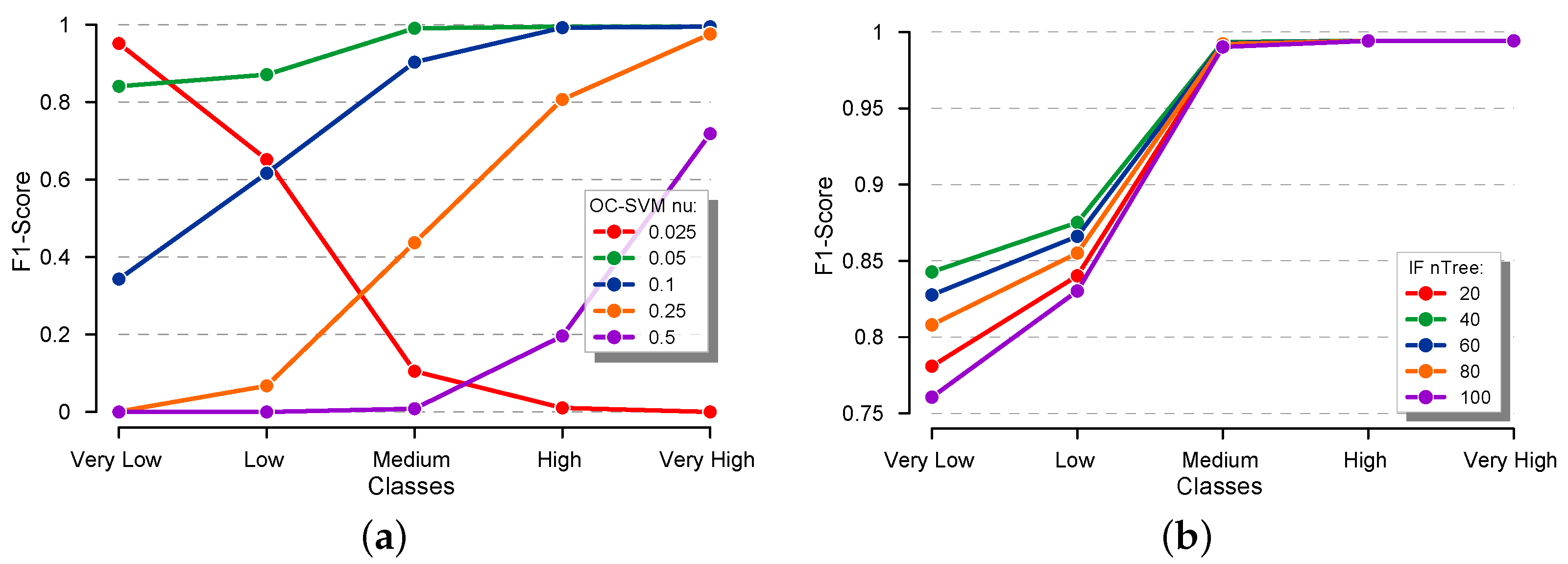
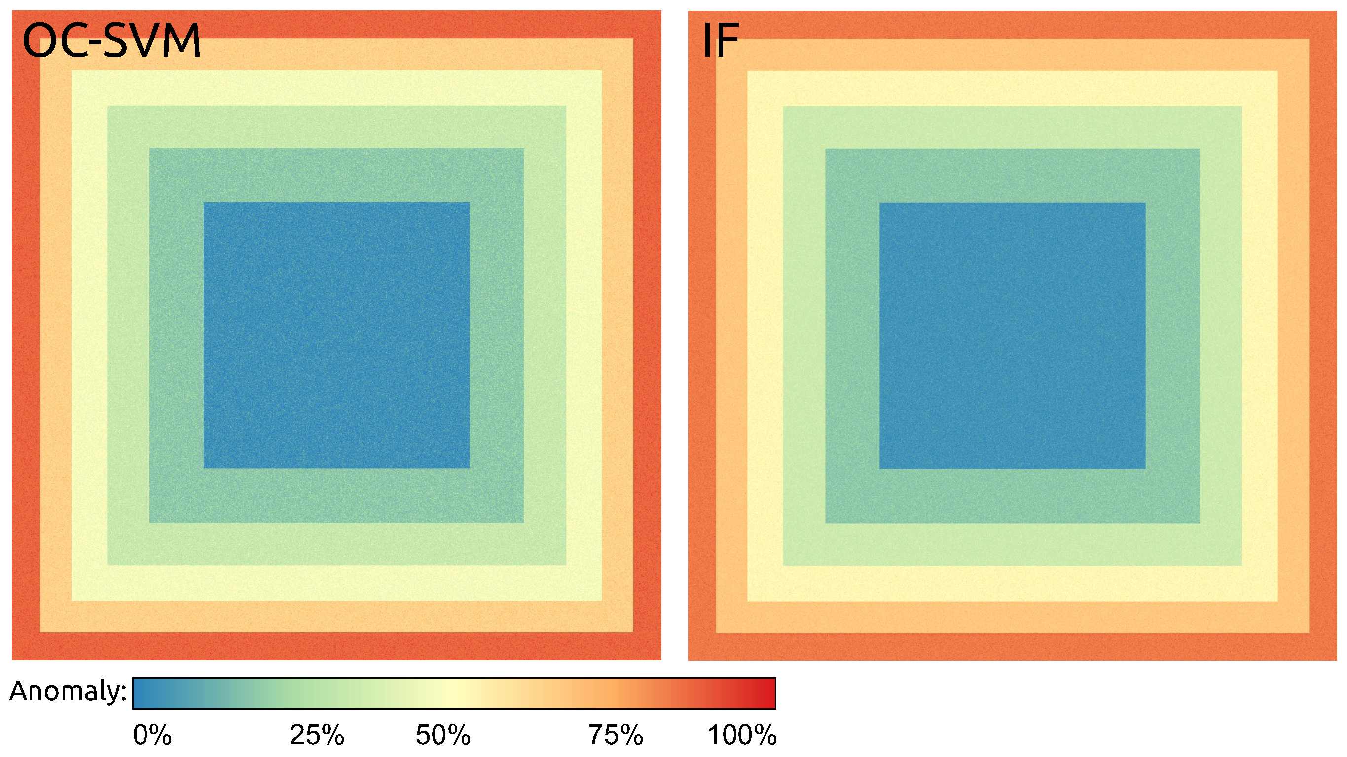
In order to assess the proposed framework, this section presents an extensive set of experiments with synthetic data and real-world remotely sensed images. Specifically, Section 4.1 presents an experiment that used a synthetic image series with different anomaly frequencies. This experiment aims to (i) provide an initial battery of tests with controlled data to demonstrate that the proposed framework achieves the expected results in several scenarios of applications (i.e., distinct anomaly frequencies) and (ii) point out the need to tune the model with appropriate parameters. Afterward, Section 4.2 demonstrates three case studies in which the framework was applied to distinct areas, periods, and sensors. The kappa coefficient [64] and F1-score [65] were used to assess the results’ accuracy.

4.1. Synthetic Data

Firstly, the proposed framework was assessed by using a synthetic image series. Figure 2a displays the conceptual structure for an image in this series, which was segmented into six regions (red, green, blue, orange, cyan, and magenta). Formally, let ${\mathcal{I}}^{\left(i\right)}$ be an image defined on a support $\mathcal{S}$, wherein for a given position $s\in \mathcal{S}$, ${\mathcal{I}}^{\left(i\right)}\left(s\right)=x\in [-1,+1]$. Furthermore, $\mathcal{S}$ was segmented in terms of the regions ${\mathcal{R}}_1,\dots ,{\mathcal{R}}_6$ according to the following criteria: $\mathcal{S}={\bigcup }_{j=1}^6{\mathcal{R}}_j$; ${\bigcap }_{j=1}^6{\mathcal{R}}_j=\varnothing$; $\#{\mathcal{R}}_j=\#{\mathcal{R}}_{\ell },\forall j,\ell =1,\dots ,6$. From the structure obtained above, an image series ${\mathcal{I}}^{\left(1\right)},\dots ,{\mathcal{I}}^{\left(100\right)}$ was synthesized, where the value x was drawn from a uniform distribution according to the region to which s belonged. Moreover, the values x were drawn while assuming the following: If $s\in {\mathcal{R}}_j$, we had a total of $(100-20·(j-1\left)\right)$ instants where ${\mathcal{I}}^{\left(i\right)}\left(s\right)=x\in [-0.2,+0.2]$; otherwise, $x\in [-1,-0.2[\cup ]+0.2,+1]$. Figure 2b depicts values of x as observed over the time series for randomly selected positions s in each region.

After determining the image series, the proposed framework was applied to map the temporal disturbances by considering both the OC-SVM and IF methods as anomaly detection models. Based on the simulation process, we manually set the envelope to $[-0.2,+0.2]$ and used only pixels inside the region ${\mathcal{R}}_1$ (i.e., free of anomalies) to model the OC-SVM and IF methods. In our analysis, the following parameter configurations were taken: $\nu \in \{0.025,0.05,0.1,0.25,0.5\}$; $nTree\in \{20,40,60,80,100\}$. The RBF kernel function was adopted in the OC-SVM method with $\gamma =0.01$. The outputs were assessed in terms of the F1-score by using five “classes of disturbances”, which are represented herein by “very low”, “low”, “medium”, “high”, and “very high” when the anomaly frequencies were in the 1–20%, 21–40%, 41–60%, 61–80%, and 81–100% ranges, respectively. The most internal region (${\mathcal{R}}_1$—the red block in Figure 2a) was not taken into account when computing the values of the F1-score.

Figure 3 shows the performance of OC-SVM and IF on each “class of disturbance” when considering distinct parameters ($\nu$ and $nTree$). Regardless of the method or parameter, the “medium”, “high”, and “very high” classes were perfectly identified (i.e., with F1-score = 1). Conversely, the choice of the method and parameter were relevant when mapping the classes “very low” and “low”, where $\nu =0.05$ and $nTree=40$, implying good choices for OC-SVM and IF, respectively. The maps obtained with these parameter configurations are shown in Figure 4.

The results support the conclusion that both OC-SVM and IF allowed the segmentation of the full synthetic image series according to the defined “anomaly frequency classes”. It is worth noticing that the performance of the OC-SVM method was strongly influenced by the parameter $\nu$ (Figure 3a). Conversely, the IF method showed good performance in identifying the “medium”, “high”, and “very high” classes regardless of the choice of parameter $nTree$ (Figure 3b).

4.2. Real-World Applications

Experiments with actual remote sensing data are given and discussed in this section by taking distinct study areas and images acquired by different remote sensors. The study areas and corresponding datasets are discussed in Section 4.2.1, followed by the results and the analyses presented in Section 4.2.2.

In order to avoid having useless data while reducing the computational effort, we eliminated the image series whose cloud/shadow occurrences exceeded 20% of the total study area. Concerning the envelope width, after an extensive battery of experimental tests, $\alpha =0.5$ was taken as a convenient choice for (i) defining the envelope $[-\alpha \sigma ,+\alpha \sigma ]$ and (ii) selecting valid samples for training the anomaly detection methods.

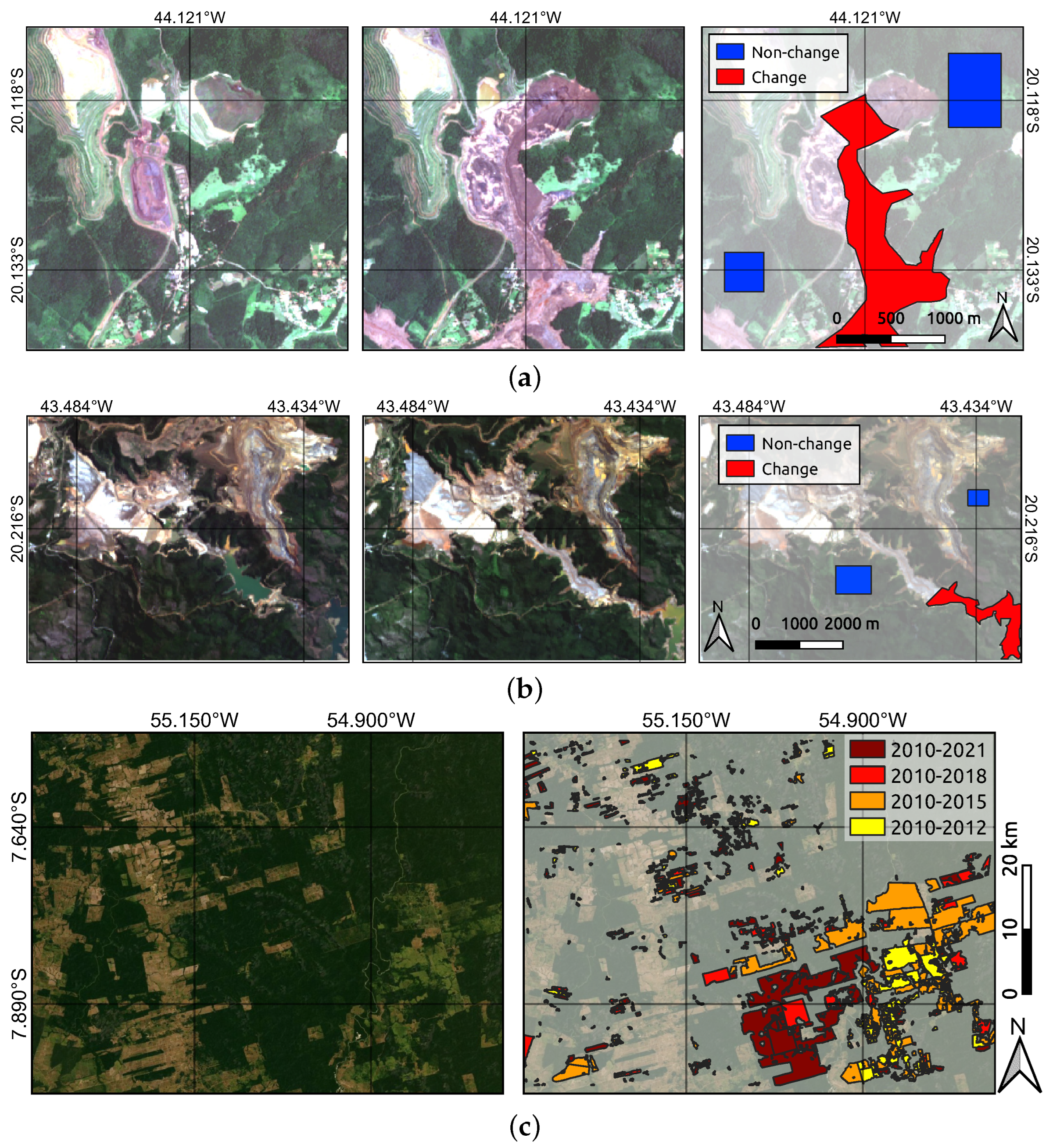
4.2.1. Study Areas and Datasets

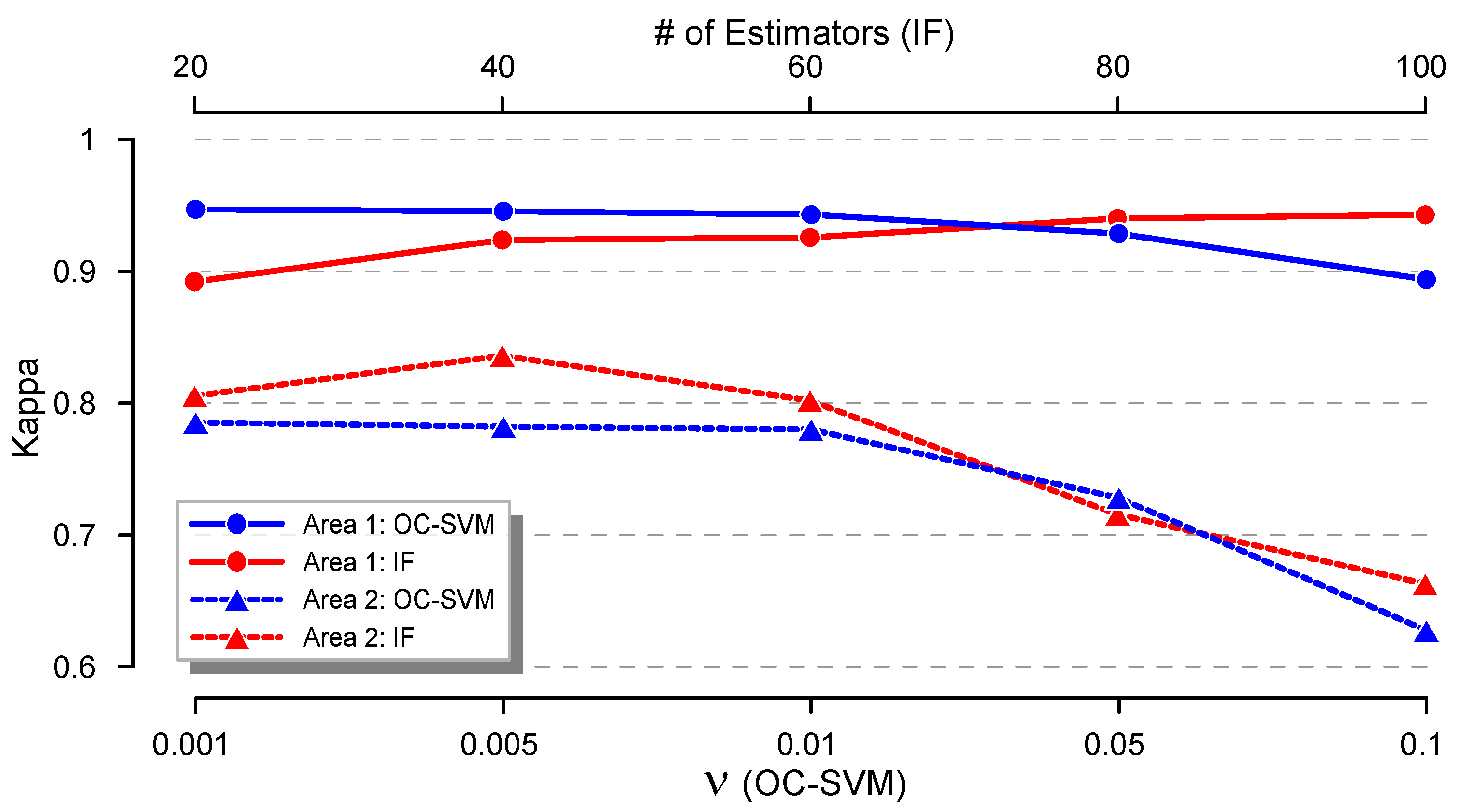
Figure 5 presents the study area locations evaluated in this experiment. The first study area (Area 1) comprised the region of Brumadinho, Minas Gerais, Brazil. This region was deeply modified after a dam collapse on 25 January 2019. The second study area (Area 2) contained the region of Mariana, Minas Gerais, which was also affected by a dam collapse on 5 November 2015. Finally, the third area (Area 3) contained a portion of Altamira, Pará, Brazil, a region under intense deforestation over the last decade. According to the Brazilian Institute of Geography and Statistics (IBGE) [66], the deforested regions located in the leftmost part of Area 3 have been continuously used for intensive cultivation/planting of soybeans and wheat, causing significant spectral variations over time every year, especially before the harvest, when the land cover is converted into bare soil. Notice that the recurrent variability in the spectral indices found in those cropped areas presents a well-known behavior, as discussed in previous applications [67,68].

Concerning the first area, a times series of 71 images acquired by the Operational Land Imager (OLI) sensor on board the Landsat-8 satellite was employed. These images had a 30 $\mathrm{m}$ spatial resolution and were acquired between 1 January 2013 and 31 December 2021. For Area 2, an image series of 62 instants was taken, ranging from 1 January 2016 to 31 December 2021 and obtained by the Multi-Spectral Instrument (MSI) on board the Sentinel-2A/B satellites with 10 $\mathrm{m}$ of spatial resolution. Finally, for Area 3, images acquired by the Moderate-Resolution Imaging Spectroradiometer (MODIS) product MOD13Q1.006 Terra Vegetation Indices 16-Day Global were adopted with 250 $\mathrm{m}$ of spatial resolution. Considering the period of analysis from 1 January 2010 to 31 December 2021, a total of 276 images were obtained. The NDVI, NDWI, and GVMI indices were considered for Areas 1, 2, and 3, respectively. This choice focused on better distinguishing the targets found in each study area—specifically, Area 1: soil and vegetation; Area 2: water, soil, and vegetation; Area 3: high- and low-biomass areas.

In order to assess the results, ground-truth reference samples were collected after a careful visual interpretation of Areas 1 and 2. These samples were divided into “non-change” and “change” areas. On the other hand, since a constant deforestation process has modified the third study area, we employed the polygons from the annual deforestation inventory provided by the well-established Monitoring Program for the Amazon and Other Biomes (PRODES) [69] as ground-truth samples. In this case, the samples were grouped into four periods: 2010–2012, 2010–2015, 2010–2018, and 2010–2021; thereafter, they were used to assess the periods 2010–2012, 2013–2015, 2016–2018, and 2019–2021. Figure 6 depicts the selected ground-truth samples for each study area.

4.2.2. Results

Considering the study areas, image series, and reference samples that were previously described, the proposed framework was then applied to map the landscape disturbances. Similarly to the experiments with synthetic data, the OC-SVM and IF methods and the distinct parameter configurations for $\nu$ and $nTree$ were tested.

Figure 7 depicts the achieved results as measured with the kappa coefficient. Regarding the OC-SVM method, one can conclude that $\nu =0.001$ led to a good parameter choice for Areas 1 and 2. On the other hand, while $nTree=40$ was shown to be a reasonable parameter for IF in Area 2, the same was not observed for Area 1, where $nTree=100$ delivered higher accuracy.

Given the most suitable parameters, as highlighted in Figure 7 (i.e., OC-SVM/$\nu$ equals $0.001$ for Areas 1 and 2; IF/$nTree$ equals 100 and 40 for Areas 1 and 2, respectively), the respective landscape disturbance maps are shown in Figure 8 and Figure 9. These maps exhibit the temporal dynamics in terms of “anomaly detection percentages”.

Complementarily, Figure 10 indicates the anomaly frequencies according to the “class of disturbances” for Areas 1 and 2. By visually inspecting the results, one can verify that both methods performed similarly in each study area. As expected, the non-changed areas tended to be assigned to very low and low anomaly frequencies.

Regarding the third study area, Figure 11 presents the accuracy values in terms of the F1-score for the periods 2010–2012, 2013–2015, 2016–2018, and 2019–2021. The OC-SVM method performed better with $\nu =0.1$. Concerning the IF method, the most accurate results were achieved with 40 trees. According to the adopted parameters, Figure 12 and Figure 13 present the landscape disturbance maps obtained with the OC-SVM and IF methods. The landscape disturbance maps agreed with the ground-truth samples in Figure 6c, mainly when focusing on the lower-right region. As already observed for Areas 1 and 2, the outputs of the OC-SVM and IF methods shared high similarities.

In addition, the best parameter configurations observed for Area 3—OC-SVM/$\nu =0.1$ and IF/$nTree=40$—were assigned to Figure 12 and Figure 13 as anomaly count maps, and the anomaly degree was divided into triennial periods according to the PRODES deforestation data.

5. Discussion

Remote sensing and machine learning tools have arisen as convenient approaches for environmental monitoring and for supporting legal decisions. Although surveillance technologies have evolved significantly in Brazil, enforcement for mining dams and deforestation has lagged since the middle of the 2010s due to the distribution and use of resources from public institutions. Therefore, this study aimed to develop a data-driven anomaly-detection-based framework for monitoring and mapping frequently disturbed areas.

In this sense, the proposed framework was applied to both the simulated dataset and areas that were recently affected by dam collapses (Areas 1 and 2) and intense deforestation (Area 3). Although the simulated dataset did not show seasonal trends, it presented anomaly occurrences with different frequencies over distinct regions. It was observed that the OC-SVM method was more sensitive to parameter changes. Given the convenient parameterization, the methods performed similarly (Figure 3). Therefore, the synthetic experiments responded as expected.

The same behavior was verified in the experiments with real-world remote sensing applications. First, regarding Areas 1 and 2, both methods identified the areas affected after the collapse of the dams (Area 1—center-bottom regions; Area 2—southeast region). Low-dynamic regions, such as those with preserved vegetation and exposed soil, were also highlighted when the proposed framework used the GVMI (Area 2) and NDWI (Area 3) indices.

Figure 12 and Figure 13 show the “anomaly count” maps for each triennial period between 2010 and 2021. Considering that the deforested areas in this region hold agricultural expansion purposes [66], leading to a recurrent crop-to-soil transition, it is expected that such areas will present “high” and “very high” disturbance class profiles over the years. In addition, one can notice that the recent agricultural activities (e.g., nearby coordinates of 54.9W/7.89S) were correctly assigned as “medium” disturbances, as the mentioned transition was not mature enough compared to that in other areas (e.g., the central-right and central-left quadrants, which were deforested between 2012 and 2015 and before 2010, respectively).

Regarding the differences observed in the outputs obtained when distinct models were adopted, we should consider that the OC-SVM and IF models follow different identification/classification schemes. While the OC-SVM method is used to identify extreme (i.e., anomalous) cases with an occurrence probability of $\nu$, the IF method exploits the divergences observed in the data so as to create a decision tree ensemble that does not necessarily establish a percentage of anomalies. Moreover, the models’ parameter tuning is another procedure that may influence the definitive classifications.

Despite their flexibility and good fitting capabilities, AD-based models also have limitations. Although anomaly-detection-driven methods allow for the mapping of concrete changes by assuming only an image time series as input data, they may not successfully capture changes under very specific circumstances, i.e., when concrete modifications occur at the end of the time series. Since the number of representative images in a given time series is an important parameter when training and modeling decision rules, a simple yet effective strategy for circumventing this issue may be to expand the number of instants of the analysis period in an effort to increase the number of anomalies to be quantified.

A practical aspect to be observed when using our approach is that there are no conceptual barriers to applying the designed methodology for the mapping of spatio-temporal dynamics in many other contexts—for example, identifying regions with recurrent changes in urban areas and landscapes with complex configurations. In those cases, a convenient spatial resolution and set of spectral indices would be provided to capture the relevant changes in the images. For instance, one may consider high-resolution data to improve the target’s discriminability—in the spirit of [70]—and then apply anomaly detection models to accurately map temporal changes.

However, it is worth mentioning that the proposed methodology may not achieve optimal performance for regions composed of low-contrast targets or those that are extremely dynamic, such as those observed in deserts and glaciers. Nonetheless, an appropriate analysis can be made for the better circumvention of this expected drawback.

6. Conclusions

This paper introduced a fully unsupervised data-driven framework for mapping landscape disturbances by combining remote sensing image series and anomaly detection methods. Experiments with simulated and real-world remote sensing data were carried out in order to demonstrate the effectiveness and robustness of the designed framework.

Based on the presented results, it was verified that the proposed methodology, which was applied as an environmental monitoring system prototype, was capable of detecting anomalies corresponding to targets with high spectral–temporal dynamics. Furthermore, both tested anomaly detection methods performed similarly after a convenient parameter choice.

In contrast to most of the methods discussed in the recent literature—e.g., the prediction of forest dynamics via spatiotemporal data fusion from multiple sources [71], multitemporal classification for agricultural landscape transformation [72], and the monitoring of land-cover dynamics via deep learning and remote sensing images [73]—our approach was designed to be data-efficient, as it does not require high-resolution or fused data, nor large labeled datasets, as demanded by deep learning schemes. Moreover, the methodology is not limited to monitoring only forest or agricultural areas. As a result, our framework could contribute to the advancement of the debate on the protection, management, and planning of landscapes, as promoted by the European Landscape Convention (ELC) [74]. Furthermore, the framework’s versatility extends beyond forest and agricultural monitoring, thus allowing researchers to gain a broader understanding of landscapes while still detecting changes in other contexts, such as deforestation or disasters. This could potentially encourage more transdisciplinary research on the impacts of landscapes in fields such as ecology and geography.

In summary, the main contributions of this paper are the following:

• A fully unsupervised framework designed to detect regions that are subject to relevant spatio-temporal disturbances. Our approach uses the Google Earth Engine platform to collect fresh data, allowing the training of data-driven models while discriminating the transient features present in time series of remotely sensed images.
• Our approach is capable of accurately identifying and mapping concrete changes by assuming only a time series of remotely sensed images as input data.
• The proposed methodology allows the use of distinct anomaly detection models, as well as image time series acquired by various remote sensors, including Landsat-8 OLI, Sentinel-2 MSI, and Terra MODIS.
• An innovative conjunction of unsupervised machine learning concepts and remote sensing techniques for the identification of recurrent changes of an arbitrary nature, which is flexible enough to address a variety of anthropogenic actions, including deforestation and landscape changes caused by disaster events, such as dam failures.

As a perspective for future work, we include (i) the assessment of the seasonal impacts, randomness, and intensity, (ii) the investigation of other specific combinations of spectral indices, including an extension for properly dealing with multiple attributes, (iii) the analysis of other anomaly detection approaches, and (iv) the evaluation of additional remote sensors, including synthetic aperture radars, hyperspectral instruments, and aerial photos.

References

1. Hawken, P.; Lovins, A.B.; Lovins, L.H. Natural Capitalism: The Next Industrial Revolution; Routledge: London, UK, 2013. [Google Scholar]
2. Steffen, W.; Broadgate, W.; Deutsch, L.; Gaffney, O.; Ludwig, C. The trajectory of the Anthropocene: The great acceleration. Anthr. Rev. 2015, 2, 81–98. [Google Scholar] [CrossRef]
3. Pradhan, P.; Costa, L.; Rybski, D.; Lucht, W.; Kropp, J.P. A systematic study of sustainable development goal (SDG) interactions. Earth’s Future 2017, 5, 1169–1179. [Google Scholar] [CrossRef] [Green Version]
4. Jimenez, J.C.; Marengo, J.A.; Alves, L.M.; Sulca, J.C.; Takahashi, K.; Ferrett, S.; Collins, M. The role of ENSO flavours and TNA on recent droughts over Amazon forests and the Northeast Brazil region. Int. J. Climatol. 2019, 41, 3761–3780. [Google Scholar] [CrossRef]
5. Silva Junior, C.H.; Pessoa, A.; Carvalho, N.S.; Reis, J.B.; Anderson, L.O.; Aragão, L.E. The Brazilian Amazon deforestation rate in 2020 is the greatest of the decade. Nat. Ecol. Evol. 2021, 5, 144–145. [Google Scholar] [CrossRef]
6. Burton, C.; Betts, R.A.; Jones, C.D.; Feldpausch, T.R.; Cardoso, M.; Anderson, L.O. El Niño driven changes in global fire 2015/16. Front. Earth Sci. 2020, 8, 199. [Google Scholar] [CrossRef]
7. Moura, M.M.; Dos Santos, A.R.; Pezzopane, J.E.M.; Alexandre, R.S.; da Silva, S.F.; Pimentel, S.M.; de Andrade, M.S.S.; Silva, F.G.R.; Branco, E.R.F.; Moreira, T.R.; et al. Relation of El Niño and La Niña phenomena to precipitation, evapotranspiration and temperature in the Amazon basin. Sci. Total Environ. 2019, 651, 1639–1651. [Google Scholar] [CrossRef] [PubMed]
8. do Carmo, F.F.; Kamino, L.H.Y.; Junior, R.T.; de Campos, I.C.; do Carmo, F.F.; Silvino, G.; Mauro, M.L.; Rodrigues, N.U.A.; de Souza Miranda, M.P.; Pinto, C.E.F.; et al. Fundão tailings dam failures: The environment tragedy of the largest technological disaster of Brazilian mining in global context. Perspect. Ecol. Conserv. 2017, 15, 145–151. [Google Scholar] [CrossRef]
9. Rotta, L.H.S.; Alcantara, E.; Park, E.; Negri, R.G.; Lin, Y.N.; Bernardo, N.; Mendes, T.S.G.; Souza Filho, C.R. The 2019 Brumadinho tailings dam collapse: Possible cause and impacts of the worst human and environmental disaster in Brazil. Int. J. Appl. Earth Obs. Geoinf. 2020, 90, 102119. [Google Scholar]
10. Hansen, M.C.; Potapov, P.V.; Moore, R.; Hancher, M.; Turubanova, S.A.; Tyukavina, A.; Thau, D.; Stehman, S.V.; Goetz, S.J.; Loveland, T.R.; et al. High-Resolution Global Maps of 21st-Century Forest Cover Change. Science 2013, 342, 850–853. [Google Scholar] [CrossRef] [Green Version]
11. Berger, K.; Machwitz, M.; Kycko, M.; Kefauver, S.C.; Van Wittenberghe, S.; Gerhards, M.; Verrelst, J.; Atzberger, C.; van der Tol, C.; Damm, A.; et al. Multi-sensor spectral synergies for crop stress detection and monitoring in the optical domain: A review. Remote Sens. Environ. 2022, 280, 113198. [Google Scholar] [CrossRef]
12. Sagan, V.; Peterson, K.T.; Maimaitijiang, M.; Sidike, P.; Sloan, J.; Greeling, B.A.; Maalouf, S.; Adams, C. Monitoring inland water quality using remote sensing: Potential and limitations of spectral indices, bio-optical simulations, machine learning, and cloud computing. Earth-Sci. Rev. 2020, 205, 103187. [Google Scholar] [CrossRef]
13. Lary, D.J.; Alavi, A.H.; Gandomi, A.H.; Walker, A.L. Machine learning in geosciences and remote sensing. Geosci. Front. 2016, 7, 3–10. [Google Scholar] [CrossRef] [Green Version]
14. Holloway, J.; Mengersen, K. Statistical machine learning methods and remote sensing for sustainable development goals: A review. Remote Sens. 2018, 10, 1365. [Google Scholar] [CrossRef] [Green Version]
15. Shaukat, K.; Alam, T.M.; Luo, S.; Shabbir, S.; Hameed, I.A.; Li, J.; Abbas, S.K.; Javed, U. A review of time-series anomaly detection techniques: A step to future perspectives. In Proceedings of the Future of Information and Communication Conference, Vancouver, BC, Canada, 29–30 April 2021; pp. 865–877. [Google Scholar]
16. Racetin, I.; Krtalić, A. Systematic review of anomaly detection in hyperspectral remote sensing applications. Appl. Sci. 2021, 11, 4878. [Google Scholar] [CrossRef]
17. Marzuoli, A.; Liu, F. Monitoring of natural disasters through anomaly detection on mobile phone data. In Proceedings of the 2019 IEEE International Conference on Big Data (Big Data), Los Angeles, CA, USA, 9–12 December 2019; pp. 4089–4098. [Google Scholar]
18. Bijlani, N.; Nilforooshan, R.; Kouchaki, S. An Unsupervised Data-Driven Anomaly Detection Approach for Adverse Health Conditions in People Living With Dementia: Cohort Study. JMIR Aging 2022, 5, e38211. [Google Scholar] [CrossRef] [PubMed]
19. Guo, Q.; Pu, R.; Cheng, J. Anomaly detection from hyperspectral remote sensing imagery. Geosciences 2016, 6, 56. [Google Scholar] [CrossRef] [Green Version]
20. Chi, M.; Plaza, A.; Benediktsson, J.A.; Sun, Z.; Shen, J.; Zhu, Y. Big data for remote sensing: Challenges and opportunities. Proc. IEEE 2016, 104, 2207–2219. [Google Scholar] [CrossRef]
21. Luz, A.E.O.; Negri, R.G.; Massi, K.G.; Colnago, M.; Silva, E.A.; Casaca, W. Mapping Fire Susceptibility in the Brazilian Amazon Forests Using Multitemporal Remote Sensing and Time-Varying Unsupervised Anomaly Detection. Remote Sens. 2022, 14, 2429. [Google Scholar] [CrossRef]
22. Hamunyela, E.; Brandt, P.; Shirima, D.; Do, H.T.T.; Herold, M.; Roman-Cuesta, R.M. Space-time detection of deforestation, forest degradation and regeneration in montane forests of Eastern Tanzania. Int. J. Appl. Earth Obs. Geoinf. 2020, 88, 102063. [Google Scholar] [CrossRef]
23. Dias, M.A.; Silva, E.A.D.; Azevedo, S.C.D.; Casaca, W.; Statella, T.; Negri, R.G. An Incongruence-Based Anomaly Detection Strategy for Analyzing Water Pollution in Images from Remote Sensing. Remote Sens. 2020, 12, 43. [Google Scholar] [CrossRef] [Green Version]
24. Nasrabadi, N.M. Hyperspectral target detection: An overview of current and future challenges. IEEE Signal Process. Mag. 2013, 31, 34–44. [Google Scholar] [CrossRef]
25. Manolakis, D.; Shaw, G. Detection algorithms for hyperspectral imaging applications. IEEE Signal Process. Mag. 2002, 19, 29–43. [Google Scholar] [CrossRef]
26. Kim, S.; Choi, K.; Choi, H.S.; Lee, B.; Yoon, S. Towards a Rigorous Evaluation of Time-Series Anomaly Detection. In Proceedings of the AAAI Conference on Artificial Intelligence, Palo Alto, CA, USA, 22 February–1 March 2022; Volume 36, pp. 7194–7201. [Google Scholar]
27. Bishop, C.M. Pattern Recognition and Machine Learning, 1st ed.; Springer: New York, NY, USA, 2007. [Google Scholar]
28. Webb, A.R.; Copsey, K.D. Statistical Pattern Recognition, 3rd ed.; John Wiley & Sons Ltd.: Hoboken, NJ, USA, 2011. [Google Scholar] [CrossRef]
29. Negri, R.G.; Frery, A.C.; Casaca, W.; Azevedo, S.; Dias, M.A.; Silva, E.A.; Alcântara, E.H. Spectral–Spatial-Aware Unsupervised Change Detection With Stochastic Distances and Support Vector Machines. IEEE Trans. Geosci. Remote Sens. 2021, 59, 2863–2876. [Google Scholar] [CrossRef]
30. Yan, J.; Wang, X. Unsupervised and semi-supervised learning: The next frontier in machine learning for plant systems biology. Plant J. 2022, 111, 1527–1538. [Google Scholar] [CrossRef]
31. Akoglu, L.; Tong, H.; Koutra, D. Graph based anomaly detection and description: A survey. Data Min. Knowl. Discov. 2015, 29, 626–688. [Google Scholar] [CrossRef] [Green Version]
32. Zhang, J.; Roy, D.; Devadiga, S.; Zheng, M. Anomaly detection in MODIS land products via time series analysis. Geo-Spat. Inf. Sci. 2007, 10, 44–50. [Google Scholar] [CrossRef] [Green Version]
33. Alvera-Azcárate, A.; Sirjacobs, D.; Barth, A.; Beckers, J.M. Outlier detection in satellite data using spatial coherence. Remote Sens. Environ. 2012, 119, 84–91. [Google Scholar] [CrossRef] [Green Version]
34. Gu, J.; Wang, L.; Wang, H.; Wang, S. A novel approach to intrusion detection using SVM ensemble with feature augmentation. Comput. Secur. 2019, 86, 53–62. [Google Scholar] [CrossRef]
35. Dereszynski, E.W.; Dietterich, T.G. Spatiotemporal models for data-anomaly detection in dynamic environmental monitoring campaigns. ACM Trans. Sens. Netw. (TOSN) 2011, 8, 1–36. [Google Scholar] [CrossRef] [Green Version]
36. Ananias, P.H.M.; Negri, R.G.; Dias, M.A.; Silva, E.A.; Casaca, W. A Fully Unsupervised Machine Learning Framework for Algal Bloom Forecasting in Inland Waters Using MODIS Time Series and Climatic Products. Remote Sens. 2022, 14, 4283. [Google Scholar] [CrossRef]
37. Ma, H.; Hu, Y.; Shi, H. Fault detection and identification based on the neighborhood standardized local outlier factor method. Ind. Eng. Chem. Res. 2013, 52, 2389–2402. [Google Scholar] [CrossRef]
38. Hoyle, B.; Rau, M.M.; Paech, K.; Bonnett, C.; Seitz, S.; Weller, J. Anomaly detection for machine learning redshifts applied to SDSS galaxies. Mon. Not. R. Astron. Soc. 2015, 452, 4183–4194. [Google Scholar] [CrossRef] [Green Version]
39. SchÖlkopf, B.; Smola, A.J. Learning with Kernels: Support Vector Machines, Regularization, Optimization, and Beyond; Adaptive computation and machine learning; MIT Press: Cambridge, MA, USA, 2002. [Google Scholar]
40. Liu, F.T.; Ting, K.M.; Zhou, Z.H. Isolation forest. In Proceedings of the 2008 Eighth IEEE International Conference on Data Mining, Pisa, Italy, 15–19 December 2008; pp. 413–422. [Google Scholar]
41. Rembold, F.; Atzberger, C.; Savin, I.; Rojas, O. Using low resolution satellite imagery for yield prediction and yield anomaly detection. Remote Sens. 2013, 5, 1704–1733. [Google Scholar] [CrossRef] [Green Version]
42. Ananias, P.H.M.; Negri, R.G. Anomalous behaviour detection using one-class support vector machine and remote sensing images: A case study of algal bloom occurrence in inland waters. Int. J. Digit. Earth 2021, 14, 921–942. [Google Scholar] [CrossRef]
43. Shawe-Taylor, J.; Cristianini, N. Kernel Methods for Pattern Analysis; Cambridge University Press: Cambridge, UK, 2004. [Google Scholar]
44. Li, S.; Zhang, K.; Duan, P.; Kang, X. Hyperspectral anomaly detection with kernel isolation forest. IEEE Trans. Geosci. Remote Sens. 2019, 58, 319–329. [Google Scholar] [CrossRef]
45. Alonso-Sarria, F.; Valdivieso-Ros, C.; Gomariz-Castillo, F. Isolation forests to evaluate class separability and the representativeness of training and validation areas in land cover classification. Remote Sens. 2019, 11, 3000. [Google Scholar] [CrossRef] [Green Version]
46. Lesouple, J.; Baudoin, C.; Spigai, M.; Tourneret, J.Y. Generalized isolation forest for anomaly detection. Pattern Recognit. Lett. 2021, 149, 109–119. [Google Scholar] [CrossRef]
47. Havil, J. Gamma: Exploring Euler’s constant. Aust. Math. Soc. 2003, 250. Available online: http://www.jstor.org/stable/j.ctt7sd75 (accessed on 3 March 2023).
48. Moreira, R.D.C. Influência do Posicionamento e da Largura de Bandas de Sensores Remotos e dos Efeitos Atmosféricos na Determinação de índices de Vegetação. Master’s Thesis, Instituto Nacional de Pesquisas Espaciais, São José dos Campos, Brazil, 2000; 181p. [Google Scholar]
49. Kaur, R.; Pandey, P. A review on spectral indices for built-up area extraction using remote sensing technology. Arab. J. Geosci. 2022, 15, 1–22. [Google Scholar] [CrossRef]
50. Rouse, J.W.; Haas, R.H.; Schell, J.A.; Deering, D.W. Monitoring vegetation systems in the Great Plains with ERTS. NASA Spec. Publ. 1974, 351, 309. [Google Scholar]
51. Xue, J.; Su, B. Significant Remote Sensing Vegetation Indices: A Review of Developments and Applications. J. Sens. 2017, 2017, 1353691:1–1353691:17. [Google Scholar] [CrossRef] [Green Version]
52. Gao, B.C. NDWI—A normalized difference water index for remote sensing of vegetation liquid water from space. Remote Sens. Environ. 1996, 58, 257–266. [Google Scholar] [CrossRef]
53. Ceccato, P.; Gobron, N.; Flasse, S.; Pinty, B.; Tarantola, S. Designing a spectral index to estimate vegetation water content from remote sensing data: Part 1: Theoretical approach. Remote Sens. Environ. 2002, 82, 188–197. [Google Scholar] [CrossRef]
54. Glenn, E.P.; Nagler, P.L.; Huete, A.R. Vegetation index methods for estimating evapotranspiration by remote sensing. Surv. Geophys. 2010, 31, 531–555. [Google Scholar] [CrossRef]
55. Sow, M.; Mbow, C.; Hély, C.; Fensholt, R.; Sambou, B. Estimation of Herbaceous Fuel Moisture Content Using Vegetation Indices and Land Surface Temperature from MODIS Data. Remote Sens. 2013, 5, 2617–2638. [Google Scholar] [CrossRef] [Green Version]
56. Zeng, J.; Zhang, R.; Qu, Y.; Bento, V.A.; Zhou, T.; Lin, Y.; Wu, X.; Qi, J.; Shui, W.; Wang, Q. Improving the drought monitoring capability of VHI at the global scale via ensemble indices for various vegetation types from 2001 to 2018. Weather Clim. Extrem. 2022, 35, 100412. [Google Scholar] [CrossRef]
57. Gorelick, N.; Hancher, M.; Dixon, M.; Ilyushchenko, S.; Thau, D.; Moore, R. Google Earth Engine: Planetary-scale geospatial analysis for everyone. Remote Sens. Environ. 2017, 202, 18–27. [Google Scholar] [CrossRef]
58. van Rossum, G.; Drake, F.L. The Python Language Reference Manual; Network Theory Ltd.: Surrey, UK, 2011. [Google Scholar]
59. Van Der Walt, S.; Colbert, S.C.; Varoquaux, G. The NumPy array: A structure for efficient numerical computation. Comput. Sci. Eng. 2011, 13, 22. [Google Scholar] [CrossRef] [Green Version]
60. McKinney, W. Data structures for statistical computing in Python. In Proceedings of the 9th Python in Science Conference, Austin, TX, USA, 28 June–3 July 2010; Volume 445, pp. 51–56. [Google Scholar]
61. Pedregosa, F.; Varoquaux, G.; Gramfort, A.; Michel, V.; Thirion, B.; Grisel, O.; Blondel, M.; Prettenhofer, P.; Weiss, R.; Dubourg, V.; et al. Scikit-learn: Machine learning in Python. J. Mach. Learn. Res. 2011, 12, 2825–2830. [Google Scholar]
62. Warmerdam, F. The geospatial data abstraction library. In Open Source Approaches in Spatial Data Handling; Springer: Berlin/Heidelberg, Germany, 2008; pp. 87–104. [Google Scholar]
63. GEE-API. Google Earth Engine API. 2022. Available online: https://developers.google.com/earth-engine (accessed on 29 October 2022).
64. Congalton, R.G.; Green, K. Assessing the Accuracy of Remotely Sensed Data; CRC Press: Boca Raton, FL, USA, 2009; p. 183. [Google Scholar]
65. Rijsbergen, C.J.V. Information Retrieval, 2nd ed.; Butterworth-Heinemann: Ann Arbor, MI, USA, 1979. [Google Scholar]
66. IBGE. Monitoramento da Cobertura e Uso da Terra. 2022. Available online: https://www.ibge.gov.br/geociencias/cartas-e-mapas/informacoes-ambientais/15831-cobertura-e-uso-da-terra-do-brasil.html (accessed on 29 October 2022).
67. Brovelli, M.A.; Sun, Y.; Yordanov, V. Monitoring Forest Change in the Amazon Using Multi-Temporal Remote Sensing Data and Machine Learning Classification on Google Earth Engine. ISPRS Int. J. Geo-Inf. 2020, 9, 580. [Google Scholar] [CrossRef]
68. Nakalembe, C.; Becker-Reshef, I.; Bonifacio, R.; Hu, G.; Humber, M.L.; Justice, C.J.; Keniston, J.; Mwangi, K.; Rembold, F.; Shukla, S.; et al. A review of satellite-based global agricultural monitoring systems available for Africa. Glob. Food Secur. 2021, 29, 100543. [Google Scholar] [CrossRef]
69. FG Assis, L.F.; Ferreira, K.R.; Vinhas, L.; Maurano, L.; Almeida, C.; Carvalho, A.; Rodrigues, J.; Maciel, A.; Camargo, C. TerraBrasilis: A spatial data analytics infrastructure for large-scale thematic mapping. ISPRS Int. J. Geo-Inf. 2019, 8, 513. [Google Scholar] [CrossRef] [Green Version]
70. Wang, X.; Liu, S.; Du, P.; Liang, H.; Xia, J.; Li, Y. Object-Based Change Detection in Urban Areas from High Spatial Resolution Images Based on Multiple Features and Ensemble Learning. Remote Sens. 2018, 10, 276. [Google Scholar] [CrossRef] [Green Version]
71. Zhu, X.; Cai, F.; Tian, J.; Williams, T.K.A. Spatiotemporal Fusion of Multisource Remote Sensing Data: Literature Survey, Taxonomy, Principles, Applications, and Future Directions. Remote Sens. 2018, 10, 527. [Google Scholar] [CrossRef] [Green Version]
72. Wang, X.; Zhang, J.; Xun, L.; Wang, J.; Wu, Z.; Henchiri, M.; Zhang, S.; Zhang, S.; Bai, Y.; Yang, S.; et al. Evaluating the Effectiveness of Machine Learning and Deep Learning Models Combined Time-Series Satellite Data for Multiple Crop Types Classification over a Large-Scale Region. Remote Sens. 2022, 14, 2341. [Google Scholar] [CrossRef]
73. Jiang, H.; Peng, M.; Zhong, Y.; Xie, H.; Hao, Z.; Lin, J.; Ma, X.; Hu, X. A Survey on Deep Learning-Based Change Detection from High-Resolution Remote Sensing Images. Remote Sens. 2022, 14, 1552. [Google Scholar] [CrossRef]
74. Pătru-Stupariu, I.; Nita, A. Impacts of the European Landscape Convention on interdisciplinary and transdisciplinary research. Landsc. Ecol. 2022, 37, 1211–1225. [Google Scholar] [CrossRef]
Figure 1. Overview of the proposed framework.
Sustainability 15 04725 g001
Figure 2. The synthesized image series. (a) The conceptual image structure. The regions R 1 , R 2 , R 3 , R 4 , R 5 , R 6 are represented in red, green, blue, orange, cyan, and magenta, respectively. (b) Values x observed for positions s selected in each conceptual image’s region. The color of each line assigns the selected position to one region.
Sustainability 15 04725 g002
Figure 3. Performance of OC-SVM and IF when identifying distinct anomaly frequency classes according to distinct parameter configurations. (a) OC-SVM. (b) IF.
Sustainability 15 04725 g003
Figure 4. Output maps obtained by the OC-SVM ( ν = 0.05 ) and IF ( n T r e e = 40 ) methods when applied to map the anomaly frequencies.
Sustainability 15 04725 g004
Figure 5. Spatial locations of the study areas.
Sustainability 15 04725 g005
Figure 6. Ground-truth reference samples for Areas 1, 2, and 3. The first two areas are represented before and after the dam collapse events. (a) Area 1—Brumadinho; Landsat-8 OLI data. (b) Area 2—Mariana; Sentinel-2 MSI data. (c) Area 3—Altamira; MODIS/MOD13Q1.006 data.
Sustainability 15 04725 g006
Figure 7. Kappa coefficient values obtained by the OC-SVM and IF methods for Areas 1 and 2 with distinct parameters.
Sustainability 15 04725 g007
Figure 8. Results for Area 1 obtained by applying the OC-SVM (left) and IF (right) methods with parameter values of ν = 0.001 and n T r e e = 100 , respectively.
Sustainability 15 04725 g008
Figure 9. Results for Area 2 obtained by applying the OC-SVM (left) and IF (right) methods with parameter values of ν = 0.001 and n T r e e = 40 , respectively.
Sustainability 15 04725 g009
Figure 10. Anomaly frequencies concerning the “non-change” and “change” ground-truth samples for Areas 1 and 2. The anomaly frequency classes are very low [ 0 % , 20 % ] , low [ 20 % , 40 % ] , medium [ 40 % , 60 % ] , high [ 60 % , 80 % ] , and very high [ 80 % , 100 % ] . (a) Area 1—OC-SVM ( ν = 0.001 ). (b) Area 1—IF ( n T r e e = 100 ). (c) Area 2—OC-SVM ( ν = 0.001 ). (d) Area 2—IF ( n T r e e = 40 ).
Sustainability 15 04725 g010
Figure 11. F1-score values obtained by the OC-SVM and IF methods for Area 3 on each analyzed period with distinct parameters.
Sustainability 15 04725 g011
Figure 12. Results for Area 3 obtained by applying the OC-SVM method with ν = 0.1 . Periods: (a) 2010–2012; (b) 2013–2015; (c) 2016–2018; (d) 2019–2021.
Sustainability 15 04725 g012
Figure 13. Results for Area 3 obtained by applying the IF method with n T r e e = 40 . Periods: (a) 2010–2012; (b) 2013–2015; (c) 2016–2018; (d) 2019–2021.
Sustainability 15 04725 g013
Disclaimer/Publisher’s Note: The statements, opinions and data contained in all publications are solely those of the individual author(s) and contributor(s) and not of MDPI and/or the editor(s). MDPI and/or the editor(s) disclaim responsibility for any injury to people or property resulting from any ideas, methods, instructions or products referred to in the content.