Article

Impact of Urbanisation on the Spatial and Temporal Evolution of Carbon Emissions and the Potential for Emission Reduction in a Dual-Carbon Reduction Context

School of Management, Suqian University, Suqian 223800, China
*
Author to whom correspondence should be addressed.
Sustainability 2023, 15(6), 4715; https://doi.org/10.3390/su15064715
Submission received: 10 January 2023 / Revised: 2 March 2023 / Accepted: 2 March 2023 / Published: 7 March 2023

Abstract

:
Urbanisation is accelerating under the new economic development trend, but the global warming exacerbated by greenhouse gases has caused a certain degree of constraint on the speed and quality of economic development, among which anthropogenic emissions, mainly from transportation, are more obvious. Therefore, based on the background of urbanisation and taking urban agglomerations as the research object, this study investigates the spatial and temporal mechanisms and dynamics of carbon emissions through the construction of carbon emission models, the identification of influencing factors, and the processing of spatial data and proposes relevant measures for carbon emission control mechanisms. This study finds that the improvement of the per capita economic level and the urbanisation rate will correspondingly lead to an increase in carbon emissions and that the spatial distribution of carbon emissions under passenger and freight transport modes shows a pattern of “low at the ends and high in the middle”, with the predicted carbon emission levels remaining balanced over a long period of time, with a variation rate of less than 1%. The model idea proposed in this study can effectively provide new perspectives and ideas for the differentiated formulation of emission reduction policies, and the government ought to focus more on the dynamic changes of urbanised carbon emissions in future development so as to realise the potential of urban emission reduction.

1. Introduction

The promotion of “double carbon” reduction (peak carbon and carbon neutral) is one of the most important initiatives to reduce the challenges posed by resource and environmental constraints and to accelerate sustainable development and economic structural transformation. Since the Party Central Committee advised the strategic goal of achieving peak and neutral carbon by 2030 and 2060, accelerating the process of carbon reduction has gradually been put on an important strategic level. At the same time, cities, as an important carrier form of economic development and civilisational activities, are the main battleground for achieving the double carbon goal. The acceleration of China’s reform process has also increased the corresponding urbanisation rate, with the average annual growth rate of urbanisation reaching a maximum of two times that of the pre-1978 period, while the total carbon emissions have increased by a factor of six [1,2]. Understanding the evolution of carbon emissions in the urbanisation process can offer a basis for the formulation of countermeasures, and at the same time, can ensure the high quality and efficiency of economic development while improving environmental quality. Therefore, this study took a coastal city group as the research target to analyse the potential of carbon emission reduction under the urbanisation process, with a view to providing reference ideas for the long-term effectiveness of a low-carbon economy.

1.1. Analysis of the Evolution Mechanism of Urbanisation and Carbon Emission and the Significance of Carbon Reduction Potential

When urbanisation reaches a certain level, it leads to a more intensive and productive use of urban land, but the carbon reduction effect is much lower than the construction content of carbon emissions. Exploring the mechanisms that influence urbanisation and carbon emissions is an important objective in line with national strategic development goals and the vision of a sustainable future for humanity [3]. Different scholars have presented different views on the carbon reduction effect of urbanisation, among which Udemba E N and others found a negative effect between economic growth and carbon emission reduction by means of least squares and lagged regression analysis and suggested that more renewable energy should be considered in the formulation of future carbon reduction policies [4]. The dual carbon targets of carbon neutrality and carbon peaking have become important external factors for China’s future energy use and economic restructuring [5]. The projection model is designed to simulate energy demand under different scenarios. Zhang C studied and analysed the overall carbon emissions and related constraints of the Yangtze River Economic Belt with the SFA model. The results showed a ‘U’ shape between industrialisation and urbanisation and carbon emissions and efficiency levels and that government intervention, regional trade, and energy consumption structure have a negative incentive effect [6]. For the sake of increasing the productivity of carbon reduction in the future, the government should insist on the restructuring of industries and the use of innovative green technologies to provide endogenous motivation for green normalisation to boost economic development.

1.2. The Impact of Urbanisation on the Spatio-Temporal Evolution Mechanism of Carbon Emissions and Their Reduction Potential

As urbanisation continues to advance, the differences in the level of urbanisation have led to the creation of urban agglomerations with a hierarchical structure and network organisation in terms of geographical space, which, as the main form of urbanisation in China, play a significant role in improving the level of industrialisation and the quality of urban development. The control of carbon emission content and the maintenance of economic growth speed will make this contradiction affect the development of a city in a virtuous circle. Hu H’s team of scholars analysed the urban agglomerations in the middle reaches of the Yangtze River; it turns out that carbon emissions still show a spatial pattern of total hotness and coldness in the east. The contribution of the economic level to the decoupling effect of carbon emissions exceeds 35%, and increasing energy intensity will increase the pressure on carbon reduction [7]. Strengthening the restructuring of energy consumption and developing green urbanism are important initiatives to effectively leverage the carbon reduction effect. In the context of the dual carbon target, Sun J et al. conducted a joint analysis of the variable influencing factors exhibited by differences in electrification rates and carbon intensity, and the panel data results make clear that the influencing factors are differentiated across regions, and different carbon intensity reduction measures should be suggested for the actual situation of different regions [8].
The form of greenhouse gas emissions caused by global warming is more severe. Wang W’s research team took the double carbon target as the research background and carried out carbon emission prediction analysis with the help of the STIRPAT model and regression analysis. They proposed regional governance mechanism and low carbonisation strategy research on obtaining the spatial variability of carbon emissions [9]. Helping promote low-carbon process can effectively ensure the coupling and coordination of urbanisation. Song Q et al. conducted a study on low carbon development based on China’s provincial data and the carbon emission–urbanisation system model, and the provincial footprint differences in their low carbon development levels are obvious, as its coordination will be affected by the geographical location [10]. In the context of international environmental constraints on carbon emission reduction, Tang Y et al. analysed the quantile point regression model of carbon emissions and found that there is an inverted U-shaped relationship between the level of urbanisation and the level of de-industrialisation and carbon emissions, and that the differentiation of emission reduction measures should be focused on at different urban development stages [11]. Meanwhile, Qi X’s empirical unpacking of the influence of population urbanisation and trade openness suggests that scale structure, technology level, and social effects can effectively play a mediating role, and that China should grasp the application of the “inverted U” relationship in emission reduction control based on the threshold effect [12]. Lv Q analysed the relationship between the drivers of freight carbon emissions and regional urbanisation using a weighted regression model [13]. The results showed that the above indicators had a non-linear relationship with the carbon emissions per capita. Furthermore, population density is proportional to the degree of aging, with a more significant reduction of carbon dioxide per capita [14]. Wang Q et al. explored the nonlinear impact of population aging on carbon emissions with the help of the panel threshold regression (PTR) model and set explanatory variables, threshold variables, and control variables. The results showed that the intensification of population aging caused an inverse U-shaped correlation between urbanisation and the carbon emissions of high-income groups [15]. Xu B et al. carried out an empirical analysis of carbon dioxide in the heavy industry with the help of a geographical weighted regression model and put forward suggestions on carbon reduction measures for regional cities according to different development conditions [16]. Qin H et al. conducted a dynamic analysis of the driving process of China’s urban carbon dioxide emissions with the help of geographical weighted regression and divided the impact degree of the driving factors by two-step clustering. The results showed that the population density and the proportion of the secondary industry were positively correlated with carbon dioxide emissions, while the number of buses per 10,000 people was negatively correlated with carbon dioxide emissions, and the spatial heterogeneity of different influencing factors was more prominent [17]. Xu G and his research team introduced the nonlinear autoregression with external input (NARX) model to the problem of carbon emission peaking and predicted carbon dioxide emissions under different scenarios with the help of a nonlinear artificial neural network. They ranked the factors affecting carbon dioxide with the help of an average impact value and put forward relevant suggestions and contents for carbon reduction [18]. Liu B explored the correlation between the urbanisation process and carbon reduction efficiency and found that population and economic effects had different impacts on carbon reduction efficiency and that there are regional differences in their efficiency [19]. Therefore, the degree of development of urban agglomerations and the mechanism of each effect should be taken into account when improving carbon efficiency in the future.

1.3. Analysis of the Spatial and Temporal Evolution Mechanisms and Dynamics of Carbon Emissions in the Context of Urbanisation

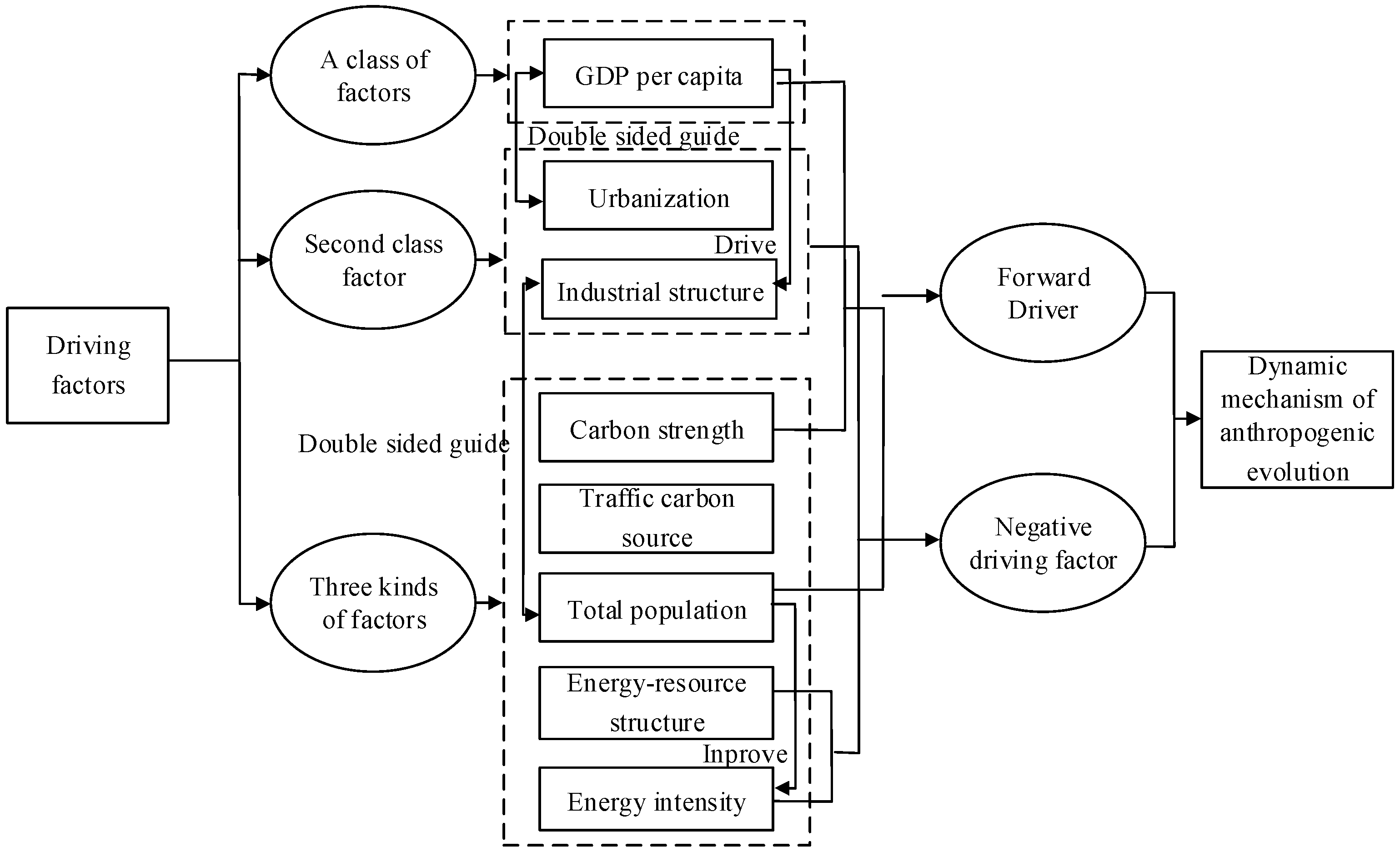
1.3.1. Model Construction for Measuring Carbon Emissions from Anthropogenic Sources

Carbon emission sources include natural carbon emission sources and anthropogenic emission sources, which mainly describe the emission process of atmospheric carbon dioxide. Because of the wide range and complexity of its sources, the main carbon emissions that cause changes in the greenhouse effect are currently anthropogenic sources. Figure 1 shows the framework of the dynamics of the evolution of carbon emissions from anthropogenic sources. It is significant to classify the factors influencing the generation of carbon emissions from anthropogenic sources into different levels and to explore the interlinkages among the influencing factors at different levels and their regulatory effects on carbon emissions so as to effectively achieve the “right remedy” for carbon reduction and regulation.
The formulation of carbon reduction policy is one of the important measures to reduce greenhouse gases. The STIRPAT model has been one of the main methods used to analyse the impact factors of carbon emissions in recent years. The variable parameters in this model include the impacts of the environment, population, GDP per capita, energy intensity, and urbanisation rate on carbon emissions from energy consumption [20]. In this study, the indicators in the model were replaced with anthropogenic source carbon emission variables, resident population, and carbon intensity to obtain the mathematical expression of the extended STIRPAT model.
Y t = α X 1 α 1 X 2 α 2 X 3 α 3 X 4 α 4 X 5 α 5
where Y is the total amount of carbon emissions, X 1 , X 2 , X 3 , X 4 , and   X 5 are the drivers of carbon emissions, representing the transport mode, carbon intensity, urbanisation level, energy mix, and industrial mix respectively, and α 1 , α 2 , α 3 , α 4 , and   α 5 are the elasticity factors of the indicator, and t is the year of time. The proportion of factors influencing the level of carbon emissions varies from city to city, which in turn requires that the carbon emission analysis is tailored to the local and temporal context. The interactions among different driving factors can effectively reveal the dynamic pattern change of urban agglomeration carbon emission efficiency [21]. In this study, spatial correlation coefficients were introduced for the analysis of carbon emission efficiency, with Moran scatter plots representing the spatial correlation of the data, where the correlation and aggregation dynamics of the variable data are represented by the spatial distributivity and correlation analysis. The mathematical expression is shown in Equation (2).
I = i = 1 n j = 1 n W i j ( x i x ¯ ) ( x y x ¯ ) / S 2 i = 1 n j = 1 n W i j I i = Z i j = 1 n W i j Z i j
where I   and   I i are the spatial autocorrelation and local autocorrelation, respectively, n is the number of spatial cells, x i   and   x y are the carbon emissions of the city unit i ,   j and x ¯ are the mean values of the variables, W i j is the contiguous space weight matrix, and Z is the normalised form of the sample space. When two urban units are adjacent, the spatial weight matrix has a value of 1 and vice versa, and when the local autocorrelation is significantly positive, it indicates that the spatial difference between the urban unit and its neighbouring city is small and vice versa. When its value is zero, it indicates that the spatial distribution of the sample spatial units shows randomness. The coefficient of variation is also used to express the relative differences among urban transport carbon emissions, and its value is positively correlated with carbon emissions. Its formula is Equation (3).
S = i = 1 n ( Y i Y ¯ ) 2 m
where m is the number of cities, and Y ¯ is the average carbon emissions. Distinct propel factors have different carbon reduction effects, and strengthening carbon emission forecasting can be an effective way to analyse carbon budgets and their reduction potential factors [22]. This study made use of the grey GM(1,1) model for carbon emission forecasting analysis, i.e., the original data columns were cumulated and new series were generated and differentiated to obtain the model GM(1,1), as in Equation (4).
X ( 1 ) ( t ) = k = 1 t X ( 0 ) ( k ) d x ( 1 ) d t + a x ( 1 ) = u
where X 1   and   X 10 are the original and cumulative data columns, respectively, n is the number of data points, n   and   a are the development factor and grey dosage, respectively, and k is the number of samples in the series. The changes in the dynamic characteristics of the different driver variables can be expressed by means of an impulse response function, which effectively responds to the standard deviation shocks caused by the perturbation of the variables over a certain period of time, and whose mathematical expression is shown in Equation (5).
Y n t = a n 1 Y n t 1 + a n 2 Y n t 1 + ε n t
where ε is the random perturbation value, and n is the number of periods.

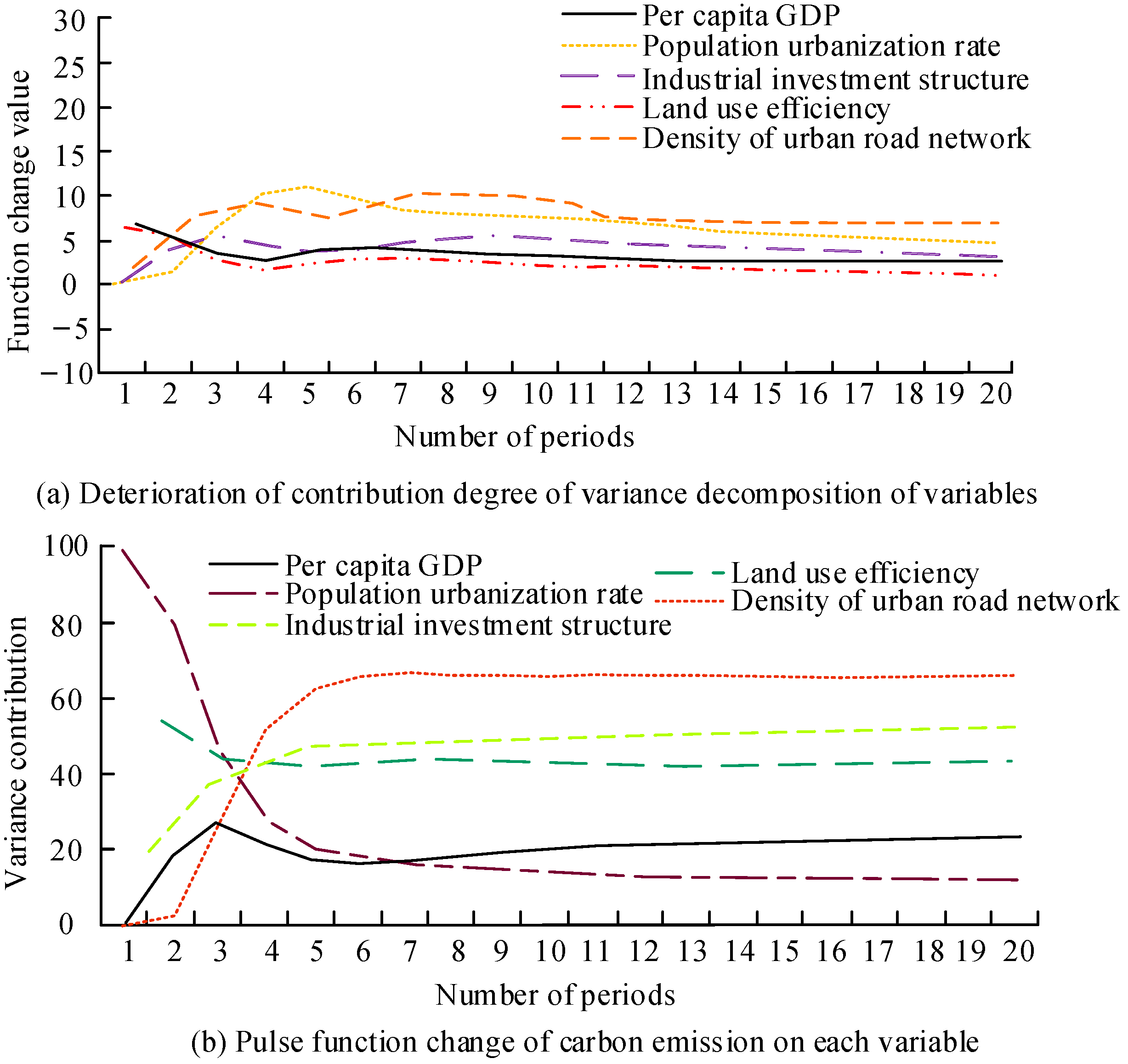
1.3.2. Analysis of Factors Influencing Carbon Emissions from Transport Sources and Construction of Regression Models

Urban expansion is one of the manifestations of urbanisation, which is manifested by an increase in construction land area, the accompanying improvement of transport networks, the deployment of related infrastructure, and the positive effect of the increased level of regional integration of urban agglomerations, which in turn leads to a spatial displacement of anthropogenic carbon emissions. Petrol and diesel are still the dominant fuels used in the transport system and have high carbon emission factors. The transport system is also subject to changes in transport demand due to technology, socio-economic development, and relevant policies [23]. The intensity of carbon emissions from different modes of transport varies, with public transport and non-motorised vehicles producing fewer carbon emissions, and adjusting the structure of intra-city passenger transport can have an optimistic constraining influence on carbon emissions. In this study, the factors that influence the carbon emissions of urban and internal transport were examined, and the significance of the dependent variable was initially removed to obtain the relevant carbon emission impact indicators.
The current mainstream transportation carbon emission measurement is the Intergovernmental Panel on Climate Change (IPCC) mobile emission source measurement, which mainly analyses the fuel data of regional transportation to obtain the carbon emissions, or the total mileage travelled by a transportation mode multiplied by the fuel consumption per unit distance travelled and then multiplied by the carbon emission factor to obtain the total carbon emissions. With the increases in traffic demand and motorisation levels, the conflict between energy saving and emission reduction in transport and the achievement of sustainable goals for low carbon cities can be better resolved. The carbon emission model for freight and passenger transport is shown in Equation (6).
C f = V i , k C F j , k r l C = S i M i N i , l r l
where C f and C are the transport carbon emissions of freight and passenger transport, respectively, j   and   k are the mode and means of transport, respectively, V i , k is the freight transport turnover, C F j , k   and   C refer to the unit energy consumption of different vehicles and the carbon emission coefficient of energy, respectively, S i is the number of i motor vehicles, M i is the mileage of motor vehicles, and N i , l is the energy consumption mileage of motor vehicles.
This study also took into account the spatial limitations of traditional linear regression models in terms of independent variables and their easier fitting properties, which make it difficult to produce better results for global estimates. Therefore, this study used the least squares method (OLS) combined with the geographical weighted regression (GWR) model to calculate the impact degree and spatial characteristics of traffic carbon emissions by indicators [24,25]. The greater the spatial correlation of factors indicates their closer proximity in terms of distance representation, and the mathematical model of the GWR model is shown in Equation (7).
y i = β 0 ( u i , v i ) + j = 1 m β j ( u i , v i ) x i j + ε i
where y i denotes the traffic carbon emissions of the city i , u i , v i are the spatial coordinates of the city i , β 0 denotes the constant term, x i j denotes the city i and the characteristic variable j , β j u i , v i is the regression coefficient of the characteristic variable, and ε i denotes the random error term that obeys normal distribution. At the same time, as the regression parameters of the samples are different, the quantity of unknown parameters far outweighs the quantity of sample points, so this study took weight values for minimising the sample size bias by means of non-parametric smoothing estimation methods, where the distance between points is inversely proportional to the weight value, i.e., the closer the distance, the larger the weight value. The weighted least squares (WLS) method can minimise the number of regression adoptions, and its mathematical expression is given in Equation (8).
i = 1 m W i j ( y i β 0 ( u i , v i ) j = 1 m β j ( u i , v i ) x i j ) 2
where W denotes the weighted correlation coefficient.
Equation (9) is the estimated value of the regression parameters.
β ( u i , v i ) = ( X i T W ( u i , v i ) X i ) 1 X i T W ( u i , v i ) Y
where X i   and   Y indicate the sets of X l k   and   y i , respectively, and W u i , v i is the diagonal matrix, with W i j as the diagonal element. The matrix is constructed to satisfy the basic principle of spatial correlation, and theoretically, there is no optimal spatial matrix. The setting of the weight values has a quantitative relationship with the spatial adjacency analysis. The GWR model differs from the linear regression model in that the regression parameters can vary with geographical location, and this study determined the degree of influence between the sample points and the observation points with the help of the weight function, whose mathematical expression is shown in Equation (10).
W i j = 1 d i j b 2 2 , d i j b 0                                       , d i j b
where W i j is the weight of the observation point i and the sample point j , d i j is the distance, and b is the non-negative decay parameter as a function between the distance and the weight. The performance of the GWR model was also tested using the information criterion method, the mathematical expression of which is shown in Equation (11).
A I C = ln R S S n + n + k n k 2
where k   and   n indicate the variables and samples, respectively, and RSS is the sum of the squared residuals. Smaller AIC values indicate better model fit performance.

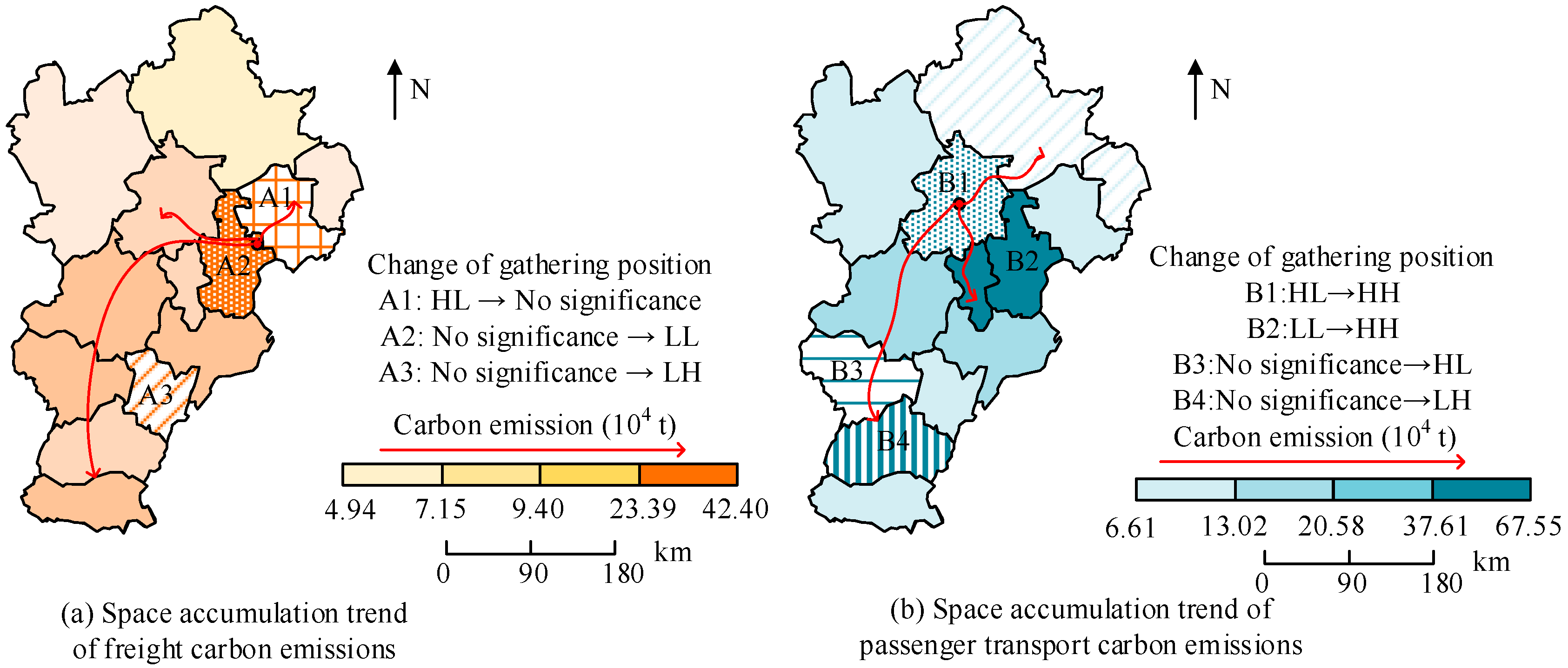
1.4. Analysis of the Spatial Change Mechanism of Carbon Emissions

1.4.1. Analysis of the Dynamics of Spatial Evolution

Common anthropogenic sources of carbon emissions include industrial energy mix, transport mix, domestic carbon emissions, waste generation, etc. This study collected statistical and analytical data on the response values of anthropogenic sources of carbon emissions for different variable factors at different periods, and the experimental data were collated through the Statistical Yearbook. The results are shown in Figure 2. The tracking period of the response function was set to five years.
Figure 2a shows the existential discrepancy in the changes in the response function curves of the variables under different periods. Specifically, there was a small fluctuation in the per capita GDP between the fourth and fifth periods, and the curve basically tended to converge after seven periods, with the resultant value of the function stabilising at 2.5. The trends of the values of the urbanisation rate, industrial investment structure, and urban transport road network before the fourth period were upward and gradually tended to be stable with the increase in the number of periods, at around 6.1, 4.8, and 7. The peak of the curve for the industrial investment structure peaked in the third period, and then the response to the shock gradually decreased after the ninth period, which was due to the high carbon emission content because of the technological lag in the early stage of industrial infrastructure construction, which gradually alleviated as the technology level rose. The urban transport factor had two small peaks in the fourth and eighth periods, with values around 8 and 10, respectively, and still had a high response to shocks in the later periods. In Figure 2b, the change in the contribution curve of all the indicators tended to level off after the sixth period, except for the indicators of the GDP per capita and the urbanisation rate, which each had a contribution of less than 30% in the later periods, and their values were all greater than 40%. The contribution curves of the industrial structure and the structure of the transport network show a high overall increase, and their degree of influence on carbon emissions was more significant, with their contribution values reaching 44% and 65% respectively, and their average growth rates reaching 1.25% and 2.38%. Therefore, controlling the carbon emission contents of transportation can validly decrease the carbon footprint and improve the low-carbon effect. The regression model was then tested for fit, where the dependent and independent variables were carbon emissions and impact factor indicators (Table 1).
The AIC is the Chichi information criterion, which can provide a standard to balance the complexity of the estimation model and the goodness of the fitting data. The AIC calculation is related to the parameter format and likelihood function of the model. The model is too complex to cause data overfitting. The AIC was the smallest, which indicates that it is less likely to be overfitted. The results in Table 1 show that the R2 of the regression model proposed in this study was low, and the AICc values displayed by it reached 100.236 and 132.206 in 2008 and 2019, respectively, which are significantly smaller than the results of the least squares model. This shows that the regression model proposed in this study has good explanatory power for the variables and its fitting ability is good. An ADF test was carried out on the influencing factors of carbon emissions, de-registering the data of each variable, and a second-order difference calculation was carried out to test the stability of the sequence. The results are shown in Table 2.
In Table 2, Ln-Carbon emissions is the explanatory variable, and Ln-GDP per capita, Ln-Urbanisation rate, Ln-Construction of traffic network, Ln-Construction of traffic network, and Ln-Energy intensity are the explained variables. The ADF test expands on the DF test. A time series is generated by the high-order autoregressive process. The ADF is a unit root test, which refers to whether there is a unit root in the test sequence, because the existence of a unit root indicates a non-stationary time series. Unit root refers to the unit root process. It can be proved that if there is a unit root in the sequence, the process is unstable, which will lead to false regression in the regression analysis. The regression results of different variable factors in Table 2 were tested by ADF, and the values obtained were all critical values under 5% and 10%, indicating that the corresponding variable difference sequence was a stationary sequence and convergent. The ADF test value of the explained variable energy consumption was the smallest and stable at the critical value. The results in the table show that energy consumption has the most obvious impact on carbon emissions. The unit root test was then performed on the sequence of energy consumption, and the results are shown in Table 3.
In Table 3, the calculation of the R code language with energy consumption as a variable shows that the ADF test value had good stability at the 5% critical value, which indicates that the data series under this variable passed the unit root test. Combining Table 2 and Table 3, it can be seen that the transportation industry has the largest elastic coefficient of energy carbon emissions. The model was also analysed descriptively (Table 4).
What can be seen in Table 4 is that in 2008 and 2012, the regression coefficients of the transport road construction were negative, and their average values were −1.06545 and −3.02132, respectively, while in 2016 and 2020, the regression coefficients of the transport factor were positive, indicating that the positive effect of indicators on carbon emissions is increasing. The regression coefficient of the industrial structure factor was negative only in 2008, while the regression values of the GDP per capita, urbanisation rate, and energy intensity indicators were positive, and there were differences in the extent of their positive effects. The median values for the GDP per capita, urbanisation rate, and energy intensity in 2020 were 0.017537, 3.236121, and 0.004966, respectively, while the mean values were 0.018718, 3.204158, and 0.006264. The variability of the coefficients indicates that the degree of influence of the impact factors on carbon emissions is governed by the spatial location of the different sample points. Therefore, the extent to which the spatiality of the impact indicators affects carbon emissions should be considered in the urbanisation process.
To further analyse the spatial area of transport carbon emissions, the spatial correlation between the two modes of transport was examined, and Table 5 was generated.
As can be seen in Table 5, the Moran index for the freight traffic carbon footprint in the time dimension was between −0.4 and −0.2 and negative, with the corresponding p-values below 10%, indicating a negative correlation between freight traffic carbon emissions and urban space. This means that the carbon emissions from freight traffic decreased as time increased, while the increasing value of the Moran index also indicates that the spatial variability of the freight traffic carbon footprint in the city decreased, and the spatial interaction tended to increase significantly. The Moran index for passenger transport was positive and exceeded 0.25, with a clear spatial aggregation effect and a positive correlation, indicating that the spatial correlation of the passenger transport carbon footprint in the city was more obvious. However, it is worth noting that the positive correlation shown by passenger transport was weak, so further attention should be paid to the dynamics of passenger transport carbon emissions for a positive effect. To further explore the spatial regions of the transport carbon footprints, the experimental data were visualised and analysed, and the results are shown in Figure 3.
As shown in Figure 3, the temporal changes in the carbon footprint of freight transport in the urban agglomeration were mainly reflected in the higher carbon emission area concentrated in the southwestern part of the urban agglomeration, where the overall carbon emissions were lower, with average carbon emissions of 8.37 × 10⁴ t, and the spatial signature of the transport carbon emissions within the city show a decrease from the centre to the surrounding area. The spatial agglomeration of the city is reflected in A1–A3, where the spatial agglomeration of A1 changed from high–low (HL) agglomeration to no significant change, and the spatial polarisation phenomenon was reduced. The spatial agglomeration of A2 changed from no significant to low–low (LL) agglomeration, and a certain degree of spatial characteristics is revealed, indicating that the spatial polarisation was more pronounced in the neighbouring areas of the city, where the carbon emissions from freight transport were higher than in this area. In the figure, the carbon footprint of passenger transport shows a decreasing trend from the centre to the periphery over time, with areas B1–B4, which had significant carbon emission changes and are mostly situated in two regions, still maintaining a high agglomeration trend. The B3–B4 region also changed from a non-agglomeration spatiality to HL and LH regions, indicating that there is an uneven spatial urban distribution of passenger transport, and two spatial effect patterns of polarisation and diffusion exist.

1.4.2. Analysis of Carbon Emission Projections and Reduction Potential

However, there is a certain degree of uncertainty and complexity in future development, so in this study, scenarios were proposed for the future growth of urban agglomerations, and their carbon reduction potential was analysed. For the prediction of carbon emissions, this study processed the original data series, obtained the baseline series, and designed a high-carbon scenario and a low-carbon scenario for data prediction. In this study, 2015–2020 was set as the baseline scenario based on the outline of the plan, and the urbanisation rate of this urban agglomeration was considered to be above 40%, assuming high- and low-carbon scenarios for the baseline scenario. At the same time, the GM (1,1) model is used to simulate the data, and the contents in Table 6 are obtained.
The results in Table 6 show that the error values between the experimentally simulated scenarios and the actual values were relatively small, basically not exceeding 1%, and the minimum error reached 0.136%, indicating that the model had a good ability to subsequently simulate the data under different carbon emission scenarios, as shown in Table 7.
In Table 7, the projected carbon emissions of this urban agglomeration under the high-carbon scenario show an increasing trend, with a relatively stable growth rate, and reaching 344,482,500 tonnes in 2041; under the low-carbon scenario, the projected carbon emissions of this urban agglomeration are less different from the baseline value, and the carbon emission efficiency decreases under the time effect, reaching 314,995,700 tonnes in 2031. The above results indicate that this urban agglomeration as a whole has a high potential for emission reduction and can effectively contribute to the improvement of environmental quality as a driving mechanism.

1.4.3. Analysis of Carbon Emission Regulation Mechanisms and Study of Strategies

The analysis of the anthropogenic sources of urban agglomeration shows that there is potential to reduce emissions by 25.402 million tonnes and 39.2716 million tonnes, and that the adjustment of unreasonable structures can effectively regulate carbon emissions. With the help of model decomposition, it can be seen that the contributions of industrial structure and transport network structure to carbon emissions are 44% and 65%, respectively, with average growth rates of 1.25% and 2%. At the same time, there is spatial variability in the regression values of the GDP per capita, urbanisation rate, and energy intensity indicators, and the negative effect of transport network construction on carbon emissions is more obvious. Therefore, this city cluster should actively facilitate the optimisation of the economic structure and the application of high-tech means in the context of the development of “carbon trading”, accelerating the clean utilisation of energy, and promoting the depth and refinement of “carbon emission reduction” products. In the context of carbon emissions, the sources of source carbon emissions are relatively extensive. Urban agglomerations should not only take into account the environmental pressure caused by traffic carbon emissions but also deepen technological upgrading, effectively control the consumption of high-carbon energy, that is, strengthen the degree of interaction between the science and technology industry and the service industry, and actively seek new manufacturing industries at the high end of the value chain, with high technology content and high added value. According to the geographical location and resource endowments of different cities, the sub-regional analysis of a carbon emission reduction control strategy was carried out. The consumption of fossil energy has become an important factor influencing the effectiveness of carbon reduction in recent years. This study analysed the carbon emissions from passenger and freight transport modes and found that the carbon emissions from freight transport had a negative correlation with urban space, while the positive correlation of carbon emissions from passenger transport had a significant spatial aggregation effect. Moreover, there is a problem of uncoordinated spatial development of urban transportation carbon emissions, and the polarisation effect of freight transportation is more prominent. Therefore, in the formulation of future transportation emission reduction and control strategies, the spatial nature of urban areas and the rationality of transportation road network planning should be considered, and the use of new energy transportation modes should be improved to reduce carbon emissions. The specific performance goal is to improve manufacturing technology in terms of the vehicle fuel economy to reduce the unnecessary waste of engine thermal efficiency and rotating systems, to subsidise new energy vehicles to expand the market share of new energy vehicles, to inhibit the role of carbon emissions from the transportation industry a certain extent, and to achieve the construction and perfection of an urban transportation system. At the same time, we will further optimise the resource allocation of different inter-city transportation mode networks and realise traffic convenience based on the carrying capacity of the resource environment and the urban space volume ratio on the basis of improving the urban function distribution. This can also balance the spatial distribution of traffic flow according to weather conditions and high and low peak periods of travel, and reasonably allocate urban traffic resources. With the continuous development of the integration of urban agglomeration, the connection of intercity transport will be strengthened, and passenger transport will become the main source of transport carbon emissions. Governments can regulate the selection of vehicle types and vehicles by issuing policy documents and declaring certain policy preferences. Each city should adjust their measures to the local conditions, formulate differentiated transport carbon emission reduction plans, increase macro-control and local benefits, and formulate different emission reduction plans according to the characteristics and current situation of urban development. The burgeoning of carbon reduction and control strategies in the context of urbanisation should be based on the micro- and meso-levels of regional development and the spatial nature of carbon emissions, for the reason of effectively accelerating the realisation of the dual carbon goals and the promotion of a low-carbon economy.

1.5. Outlook

The development of infrastructure has contributed to China’s urbanisation and has inevitably increased the burden of high consumption, with industry, construction, and transport being the main carbon generators. At the same time, the carbon emissions from waste caused by the increase in population cannot be underestimated, further making the realisation of a low-carbon economy in China difficult and challenging. A possible method to cut down carbon emissions is to accelerate the construction of low-carbon urbanisation. Carbon emission impact indicators and their spatial dynamics can provide new inspiration and ideas for the formulation of relevant strategies. This study took urban agglomeration as the research object, and through model construction and spatial and temporal evolution analysis, it was found that an increase in the urbanisation rate and the adjustment and optimisation of transport structure can advance the achievement of the carbon reduction goals. However, as there are many factors influencing carbon emissions, and the variability and complexity of these factors vary over time, future research needs to refine the analysis and account for the factors influencing carbon reduction. A wise measurement model should be built with the help of multiple information tools in order to clarify regional carbon reduction lists and the effectiveness of carbon reduction strategies. At the same time, the endogenous carbon reduction mechanism of carbon trading can advance the achievement of the dual carbon goals and sustainable economic development under the urbanisation process.

Author Contributions

Investigation, J.L. and B.L.; writing—original draft, C.Z.; supervision, P.X. All authors have read and agreed to the published version of the manuscript.

Funding

This research received no external funding.

Institutional Review Board Statement

Not applicable.

Informed Consent Statement

Not applicable.

Data Availability Statement

All data generated or analysed during this study are included in this published article.

Conflicts of Interest

The authors declare no conflict of interest.

References

  1. Buck, H.J. Mining the air: Political ecologies of the circular carbon economy. Environ. Plan. E Nat. Space 2022, 5, 1086–1105. [Google Scholar] [CrossRef]
  2. Chen, S.; Mao, H.; Sun, J. Low-carbon city construction and corporate carbon reduction performance: Evidence from a quasi-natural experiment in China. J. Bus. Ethics 2022, 180, 125–143. [Google Scholar] [CrossRef]
  3. Chen, J.; Wang, L.; Li, Y. Research on the Impact of Multi-dimensional Urbanization on China’s Carbon Emissions under the Background of COP21. J. Environ. Manag. 2020, 273, 111123. [Google Scholar] [CrossRef]
  4. Udemba, E.N.; Philip, L.D.; Emir, F. Performance and sustainability of environment under entrepreneurial activities, urbanization and renewable energy policies: A dual study of Malaysian climate goal. Renew. Energy 2022, 189, 734–743. [Google Scholar] [CrossRef]
  5. Fan, J.; Wang, J.; Liu, M.; Sun, W.; Lan, Z. Scenario simulations of China’s natural gas consumption under the dual-carbon target. Energy 2022, 252, 124106. [Google Scholar] [CrossRef]
  6. Zhang, C.; Chen, P. Industrialization, urbanization, and carbon emission efficiency of Yangtze River Economic Belt-empirical. Environ. Sci. Pollut. Res. 2021, 28, 66914–66929. [Google Scholar] [CrossRef]
  7. Hu, H.; Lv, T.; Zhang, X.; Fu, S.; Geng, C.; Li, Z. Spatiotemporal dynamics and decoupling mechanism of economic growth and carbon emissions in an urban agglomeration of China. Environ. Monit. Assess. 2022, 194, 616. [Google Scholar] [CrossRef]
  8. Sun, J.; Guo, X.; Wang, Y.; Shi, J.; Zhou, Y.; Shen, B. Nexus among energy consumption structure, energy intensity, population density, urbanization, and carbon intensity: A heterogeneous panel evidence considering differences in electrification rates. Environ. Sci. Pollut. Res. 2022, 29, 19224–19243. [Google Scholar] [CrossRef]
  9. Wang, W.; Chen, H.; Yang, R.; Wang, B.; Yang, Y. Spatial and Temporal Prediction of Carbon Peaking Goals and Zonal Governance Approaches to Achieve Carbon neutrality-A Case Study from Zhejiang Province, China. In Proceedings of the 2022 International Conference on Green Building, Civil Engineering and Smart City, Guilin, China, 8–10 April 2022; Springer: Singapore, 2022; Volume 211, pp. 151–165. [Google Scholar]
  10. Li, Y.; Li, Y.; Zhou, Y.; Shi, Y.; Zhu, X. Investigation of a “coupling model” of coordination between low-carbon development and urbanization in China. Energy Policy 2018, 121, 346–354. [Google Scholar]
  11. Tang, Y.; Zhu, H.; Yang, J. The asymmetric effects of economic growth, urbanization and deindustrialization on carbon emissions: Evidence from China. Energy Rep. 2022, 8, 513–521. [Google Scholar] [CrossRef]
  12. Qi, X.; Han, Y.; Kou, P. Population urbanization, trade openness and carbon emissions: An empirical analysis based on China. Air Qual. Atmos. Health 2020, 13, 519–528. [Google Scholar] [CrossRef]
  13. Lv, Q.; Liu, H.; Yang, D.; Liu, H. Effects of urbanization on freight transport carbon emissions in China: Common characteristics and regional disparity. J. Clean. Prod. 2019, 211, 481–489. [Google Scholar] [CrossRef]
  14. Wang, Q.; Li, L. The effects of population aging, life expectancy, unemployment rate, population density, per capita GDP, urbanization on per capita carbon emissions. Sustain. Prod. Consum. 2021, 28, 760–774. [Google Scholar] [CrossRef]
  15. Wang, Q.; Wang, L. The nonlinear effects of population aging, industrial structure, and urbanization on carbon emissions: A panel threshold regression analysis of 137 countries. J. Clean. Prod. 2021, 287, 125381. [Google Scholar] [CrossRef]
  16. Xu, B.; Lin, B. Investigating the differences in CO2 emissions in the transport sector across Chinese provinces: Evidence from a quantile regression model. J. Clean. Prod. 2018, 175, 109–122. [Google Scholar] [CrossRef]
  17. Qin, H.; Huang, Q.; Zhang, Z.; Lu, Y.; Li, M.; Xu, L.; Chen, Z. Carbon dioxide emission driving factors analysis and policy implications of Chinese cities: Combining geographically weighted regression with two-step cluster. Sci. Total Environ. 2019, 684, 413–424. [Google Scholar] [CrossRef]
  18. Xu, G.; Schwarz, P.; Yang, H. Determining China’s CO2 emissions peak with a dynamic nonlinear artificial neural network approach and scenario analysis. Energy Policy 2019, 128, 752–762. [Google Scholar] [CrossRef]
  19. Liu, B.; Tian, C.; Li, Y.; Song, H.; Ma, Z. Research on the effects of urbanization on carbon emissions efficiency of urban agglomerations in China. J. Clean. Prod. 2018, 197, 1374–1381. [Google Scholar] [CrossRef]
  20. Sun, Y.; Li, H.; Andlib, Z.; Genie, M.G. How do renewable energy and urbanization cause carbon emissions? Evidence from advanced panel estimation techniques. Renew. Energy 2022, 185, 996–1005. [Google Scholar] [CrossRef]
  21. Lai, S.; Lu, J.; Luo, X.; Ge, J. Carbon emission evaluation model and carbon reduction strategies for newly urbanized areas. Sustain. Prod. Consum. 2022, 31, 13–25. [Google Scholar] [CrossRef]
  22. An, Q.; Sheng, S.; Zhang, H.; Xiao, H.; Dong, J. Research on the construction of carbon emission evaluation system of low-carbon-oriented urban planning scheme: Taking the West New District of Jinan city as example. Geol. Ecol. Landsc. 2019, 3, 187–196. [Google Scholar] [CrossRef]
  23. Xu, Q.; Yang, R. The sequential collaborative relationship between economic growth and carbon emissions in the rapid urbanization of the Pearl River Delta. Environ. Sci. Pollut. Res. 2019, 26, 30130–30144. [Google Scholar] [CrossRef] [PubMed]
  24. Majeed, M.T.; Tauqir, A. Effects of urbanization, industrialization, economic growth, energy consumption, financial development on carbon emissions: An extended STIRPAT model for heterogeneous income groups. Pak. J. Commer. Soc. Sci. (PJCSS) 2020, 14, 652–681. [Google Scholar]
  25. Abbasi, M.A.; Parveen, S.; Khan, S.; Kamal, M.A. Urbanization and energy consumption effects on carbon dioxide emissions: Evidence from Asian-8 countries using panel data analysis. Environ. Sci. Pollut. Res. 2020, 27, 18029–18043. [Google Scholar] [CrossRef]
Figure 1. Dynamic mechanism framework for the evolution of anthropogenic carbon emissions.
Sustainability 15 04715 g001
Figure 2. Pulse function change in carbon emissions for different variable factors and analysis of their contribution.
Sustainability 15 04715 g002
Figure 3. Spatial clustering change pattern of passenger and freight transport carbon emissions in 2008 and 2018.
Sustainability 15 04715 g003
Table 1. Model test results of anthropogenic carbon emissions.
VariableRegression Model Least Squares Model
Particular YearParticular Year
2008201920082019
R20.714260.836130.58720.6753
Correction value0.613280.821490.57410.6184
AICc100.236132.206112.615146.451
Table 2. ADF test results.
VariableADF Test ValueCritical ValueStability of Critical Value
5%10%5%10%
Ln-GDP per capita−5.8678−4.1919−3.5484StableStable
Ln-Urbanisation rate−3.4121−3.2975−2.6712StableStable
Ln-Construction of traffic network−3.6344−3.8696−3.4366UnstableStable
Ln-Industrial structure−4.2687−4.2361−3.214StableStable
Ln-Energy intensity−7.8535−4.1941−3.1383StableStable
Ln-Carbon emissions−7.9128−4.254−3.1509StableStable
Table 3. Unit root test of sequence R.
VariableADF Test ValueCritical ValueStability of Critical Value
5%5%
R−5.9264−4.1032Stable
Table 4. Description of statistical analysis results of anthropogenic carbon emission model.
Particular YearIndicator VariableMinimumAverageUpper QuartileMedianLower Quartile
2008GDP per capita5.9669847.2349746.3836957.2787177.965187
Urbanisation rate0.3435850.4437420.4010380.4442570.476837
Construction of traffic network−1.28616−1.06545−1.17016−1.09939−0.96977
Industrial structure−2.089422−2.090591−2.090026−2.09048−2.0909
Energy intensity1.2212071.2220111.2214581.2218161.2224
2012GDP per capita1.888381.8944611.8920811.895171.896353
Urbanisation rate0.1021610.544440.3476250.5664810.686907
Construction of traffic network−3.025−3.02132−3.02274−3.02119−3.02004
Industrial structure0.7733841.1724861.0287651.208721367383
Energy intensity1.4530511.4540191.4535941.4539681.454436
2016GDP per capita2.6052583.2051142.7434773.1908313.58422
Urbanisation rate0.0143370.0233350.0162080.0216580.030056
Construction of traffic network0.0240880.0293150.0262460.0291590.032167
Industrial structure0.5111290.5118350.5115380.5118940.512102
Energy intensity0.0992680.1073960.1071850.1174590.118547
2020GDP per capita0.013510.0187180.004880.0175370.044421
Urbanisation rate2.5866383.2041582.8956923.2361213.458852
Construction of traffic network1.0763891.6220781.1869791.6756262.012508
Industrial structure0.0267620.0327840.0304450.0322540.036196
Energy intensity0.00330.0062640.0021960.0049660.010872
Table 5. Spatial correlation test of carbon emissions from passenger and freight transport.
Mode of TransportationParticular YearMoran IndexVarianceZ Valuep Value
Freight transport2008−0.3657370.0089123.8083060.086382
2009−0.3871470.0088984.0347940.086349
2010−0.3936460.0088944.1037400.086344
2011−0.3603750.0088973.7549490.086344
2012−0.3280910.0088813.4152160.086396
2013−0.3206480.0088863.3423340.086590
2014−0.3515840.0088693.6652870.086675
2015−0.3427440.0088273.5763130.086425
2016−0.2436320.0088044.6449820.086367
2017−0.254160.0088004.7618510.086331
2018−0.2670690.0088004.8989890.086331
2019−0.2670690.0088004.8989890.086330
2020−0.2670710.0088054.8989850.086310
Passenger transport20080.2709970.0069232.8083060.046347
20090.2728910.0069073.0347940.046355
20100.2779960.0069053.1037370.046368
20110.2660910.0069502.7549490.046346
20120.2637010.0069202.4152160.046480
20130.3064280.0068752.3423340.046540
20140.3273640.0069302.6652870.046367
20150.3285240.0068872.5763130.046376
20160.3490420.0068533.6449820.046341
20170.3399050.0068353.2667230.046356
20180.3499980.0067892.8983370.046331
20190.3620620.0067873.0202080.046330
20200.3716540.0068913.0126090.046325
Table 6. Analysis of experimental data simulation results.
Test NumberActual ValueAnalogue ValueError (%)
120,943.25620,939.8890.582
221,522.16921,521.8020.236
323,281.64723,279.2810.227
425,403.16625,416.7990.136
525,432.64825,398.2810.248
626,073.21426,066.8470.273
726,613.8972641.5310.384
Table 7. Anthropogenic source emissions under different forecast scenarios (10,000 tons).
Particular YearBaseline ScenarioHigh-Carbon ScenarioLow-Carbon Scenario
201729,181.9428,337.2628,765.90
201830,632.2528,701.2629,020.62
201931,169.1429,055.3629,437.65
202032,133.9129,399.4629,777.43
202133,127.6329,733.5430,111.93
202233,809.9830,057.5830,490.52
202334,331.9730,371.6030,680.21
202434,685.1830,675.6430,777.23
202535,041.9330,969.7730,875.73
202635,222.0831,254.0730,975.74
202735,311.6131,528.6631,077.29
202835,346.9431,793.6731,180.42
202935,377.4932,049.2431,285.15
203035,403.9132,295.5231,391.52
203135,426.7332,532.7031,499.57
203235,690.0132,760.9631,325.38
203335,139.8132,980.4931,061.21
203434,590.8633,191.5030,900.50
203533,793.6533,394.2030,875.79
203633,663.7133,588.8030,851.24
203732,534.9533,775.5430,826.87
203832,407.3433,954.6130,778.60
203932,280.8834,126.2830,754.71
204032,031.3434,290.7530,730.99
204131,908.2334,448.2530,707.42
Disclaimer/Publisher’s Note: The statements, opinions and data contained in all publications are solely those of the individual author(s) and contributor(s) and not of MDPI and/or the editor(s). MDPI and/or the editor(s) disclaim responsibility for any injury to people or property resulting from any ideas, methods, instructions or products referred to in the content.

