Abstract
This paper proposes a probabilistic hill-climbing algorithm, called PH, for the single-source transportation problem (STP). PH is a tree search algorithm in which each node contains an assignment problem (AP) transformed from the STP being solved. The transformation converts each source’s product units into product lots; a product lot equals multiple product units. The AP aims to find the optimal assignment of product lots to destinations to minimize the total assignment cost. PH uses the Hungarian method to find the optimal solution of the AP in every node, which is a solution of the STP. For the AP of the root node (as the initial current node), the number of each source’s product lots is set to be small enough to guarantee the generation of a feasible solution for the STP. To generate every subsequent level, the current node is branched into multiple child nodes, in which the number of child nodes equals the number of sources in the STP. The AP of each child node is modified from the AP of the current node by adding one more product lot into a specific different source. Consequently, each child node provides a solution that is better than or the same as the current node’s solution; however, some child nodes’ solutions may be infeasible for the STP due to the insufficiency of a source’s capacity. If all of the child nodes cannot find a better feasible solution than the current node’s solution, PH stops its procedure. To diversify the search, PH selects one of the child nodes as the new current node in a probabilistic way, instead of always selecting the best child node. The experiment’s results in this paper reveal the performance of the three variants of PH.
1. Introduction
The transportation problem (TP) [] involves shipping identical product units from sources (e.g., warehouses) to destinations (e.g., retail stores). Each source contains a specific number of product units in stock (its capacity), and it cannot supply more than its capacity. Each destination requires a specific number of product units, called the demand, and it must receive an equal number of units to the demand. Each source can supply its product units in stock to one or more destinations. Likewise, each destination can receive its required product units from one or more sources. The TP predetermines the unit transportation cost from each source to a specific destination. The TP aims to find the numbers of product units shipped from sources to destinations that minimize the total transportation cost.
The assignment problem (AP) [] is a variant of the TP. It involves assigning distinct items (e.g., product lots) to all destinations (e.g., retail stores), in which each destination is assigned exactly one item. The AP predetermines the assignment cost of each item to a specific destination. The objective of the AP is to assign a number of items to an equal number of destinations in order to minimize the total assignment cost. If the number of all items is greater than the number of all destinations, the excess items are left unassigned. The TP becomes the AP if the source capacities and the destination demands are equal to the unity.
This paper considers the single-source transportation problem (STP), a special class of the TP in which each destination must receive all of its required product units from a single source [,,,,]. The STP is thus in between the TP and AP in its form, but it is much more difficult to solve. The complexity of the STP is NP-hard because, since its introduction in 1971 [], no polynomial-time optimal algorithm has been discovered. In addition, the generalized assignment problem (GAP) [,], a close variant of the STP, belongs to the NP-hard class in the strong sense. The difference between the GAP and STP is that each destination in the GAP may change its demand when changing its source, whereas each destination in the STP does not change its demand. Some recently published algorithms on the GAP and other resource allocation problems can be found in [,,,,,,].
The STP is close to many real-world logistics systems, such as a system of delivering banknotes from bank branches to automated teller machines (ATMs). A bank owns many bank branches and many more ATMs in a city. Each ATM requires a specific number of banknotes, and each bank branch contains a much greater number of banknotes in stock. To fulfill the demands of all the ATMs, the bank must supply banknotes from its bank branches to ATMs. Based on real cases, each ATM must receive all of its required banknotes from a single bank branch. The bank branches, ATMs, and banknotes in the given application are sources, destinations, and product units, respectively, in the STP.
To solve the STP, this paper proposes a probabilistic hill-climbing algorithm called PH. It is a tree search algorithm in which each node contains an AP transformed from the STP being solved. The transformation of the STP to the AP of each node is converting each source’s product units into product lots, in which a product lot equals multiple product units. Each AP aims to find the one-to-one assignment of product lots to all destinations that minimizes the total assignment cost. PH applies the Hungarian method to find each AP’s optimal solution, which is the STP’s solution. For the AP of the root node (as the initial current node), the number of each source’s product lots equals the maximum number of destinations sorted in descending order of demand, such that the sum of their demands does not exceed the source’s capacity. To generate every subsequent level, the current node is branched into multiple child nodes, in which the number of child nodes equals the number of sources in the STP. The AP of each child node is modified from the AP of the current node by adding one more product lot into a specific different source. PH then selects one of these child nodes as the new current node in a probabilistic way.
PH has several parts that are similar to those of the existing algorithms and other parts that are different from them. PH’s framework is similar to the general framework of hill climbing (i.e., beam Search with the beam width = 1); however, PH can provide a complete solution for the STP from its root node. PH is similar to A-S (i.e., one of the branch-and-bound algorithms in []) in that they both transform the STP being solved into an AP in the root node; however, their APs are different in the number of each source’s product lots. In A-S’s root node, the number of each source’s product lots equals the maximum number of destinations sorted in ascending order of demand, such that the sum of their demands does not exceed the source’s capacity, whereas PH sorts in descending order of demand instead. Consequently, A-S usually starts its search from the root node containing the STP’s infeasible solution due to the insufficiency of a source’s capacity, whereas PH starts its search from the root node containing the STP’s feasible solution. Besides A-S, another similar algorithm to PH is the algorithm of [], which is identical to the partial PH having only the root node.
The performance of PH is highly based on its search tree structure, which is the opposite of those used in traditional tree search algorithms, e.g., branch-and-bound [,] and beam search [,]. A traditional tree search algorithm generally starts in its root node with the relaxed problem, whose optimal solution can be solved easily but is usually infeasible for the original problem. The traditional tree search algorithm then keeps adding one more restriction in order to find some relaxed subproblems whose optimal solutions are feasible for the original problem. In contrast, PH transforms the original STP to the AP in the root node, in which the number of each source’s product lots is small enough to guarantee the generation of a feasible solution for the STP. PH then keeps adding one more product lot into a source in order to keep finding better solutions for the STP.
The remainder of this paper is divided into five sections. Section 2 provides preliminaries for PH’s development along with a statement about the STP. Section 3 provides details of PH. Section 4 presents the experiment’s setup for evaluating PH’s performance. Section 5 presents the experiment’s results and discussion. Section 6 presents a conclusion of the research findings.
2. Preliminaries
This section aims to provide preliminaries for the development of PH, the proposed probabilistic hill-climbing algorithm for the STP. To do so, this section reviews the general concept of hill climbing. This section then presents a statement about the STP and its previously published algorithms.
Hill climbing is defined as the special class of beam search, in which the beam width equals the unity [,]. Beam search [,,,,,] is a breadth-first tree search algorithm with no backtracking, in which nodes in its search tree contain partial solutions. At each level, beam search keeps only a specific number of promising nodes for branching, in which the number of promising nodes kept at each level is called the beam width. If a beam search algorithm selects these promising nodes in a probabilistic way, it is then called a probabilistic (or stochastic) beam search algorithm. In the literature, there are several probabilistic beam search and hill-climbing algorithms that have been applied in different problems [,,].
The single-source transportation problem (STP) is a special class of the transportation problem (TP) in which each destination must receive all of its required product units from a single source. The STP comes with m sources (i.e., A1, A2, …, Am) and n destinations (i.e., B1, B2, …, Bn). Each source Ai (where i = 1, 2, …, m) has a specific number of product units in stock called the capacity, which is denoted by ai. Each destination Bj (where j = 1, 2, …, n) requires a specific number of product units called the demand, which is denoted by bj. In the STP, each source can supply its product units to multiple destinations, but each destination must receive all of its required product units from only one source. The STP aims to find the numbers of product units shipped from sources to destinations that minimize the total transportation cost, in which the total transportation cost is the sum of the transportation costs of all the product units shipped. Let cij denote the unit transportation cost from source Ai to destination Bj.
In 1971, the STP was first introduced by De Maio and Roveda [] along with an implicit-enumeration approach for solving the STP. Srinivasan and Thompson [] then proposed a branch-and-bound algorithm using the TP as a relaxation of the STP. Nagelhout and Thompson [] proposed two heuristics and a branch-and-bound algorithm for solving the STP. Later, Pongchairerks [] proposed four branch-and-bound algorithms for solving the STP, namely T-B, T-S, A-B, and A-S. Note that T-B is similar to the algorithm of [] with the main difference being in their branching rules. In their nodes, T-B and T-S use the TP as a relaxation of the STP, while A-B and A-S use the AP as a relaxation of the STP. In their search trees, T-B and A-B use binary tree structures, while T-S and A-S use single-assignment tree structures. An excellent review on binary and single-assignment tree structures is given in [].
In 2014, Pongchairerks [] proposed two heuristics for the STP. The first heuristic transforms the STP being solved into the lot-shipping TP. To do so, each source’s product units are converted into product lots, in which a product lot equals multiple product units, and all the required product units of each destination are converted into a single product lot. The first heuristic then solves this TP by using the MODI method. In the second heuristic, the STP being solved is transformed into an AP. Like the first heuristic, each source’s product units are converted into product lots, in which a product lot equals multiple product units. However, the AP aims to find the assignment of product lots to destinations that minimizes the total assignment cost. The second heuristic then solves the AP by using the Hungarian method. These two heuristics always return the same solution.
3. Details of Proposed Algorithm
In brief, PH searches for the optimal solution of the STP being solved in the search tree, starting from the root node at level 0. Every node in the search tree contains an AP transformed from the STP by converting each source’s product units into product lots, in which a product lot equals multiple product units. The only difference among the APs of all nodes is the number of each source’s product lots. Every AP aims to find the one-to-one assignment of product lots to all destinations that minimizes the total assignment cost. Every AP’s optimal solution, given by the Hungarian method, can be interpreted as a solution of the STP. To move to the next level, the AP of the current node is modified to the APs for its child nodes. By taking account of the solutions’ total costs, PH selects one of the child nodes as the new current node in a stochastic way.
To generate the root node at level 0, PH transforms the STP being solved to an AP as follows: PH first generates a list of all destinations by sorting them in descending order of demand. Then, let the number of each source’s product lots equal the maximum number of destinations chosen from the top of list down, such that the sum of their demands does not exceed the source’s capacity. For each specific source–destination pair, let the assignment cost of every product lot of the source to the destination equal the source-to-destination unit transportation cost multiplied by the destination’s demand. The objective of this AP is to find the one-to-one assignment of product lots to all destinations that minimizes the total assignment cost. PH then uses the Hungarian method to find the AP’s optimal solution, which is the STP’s solution. Let the root node be PH’s initial current node.
To generate every subsequent level, PH branches from the current node into m child nodes, in which m is the number of sources in the STP. The AP of the i-th child node is modified from the AP of the current node by adding one more product lot into the i-th source (where i = 1, 2, …, m). PH uses the Hungarian method to solve the APs of these child nodes; then, PH interprets their APs’ optimal solutions as the STP’s solutions. To move to the next level, the new current node is randomly selected from candidate child nodes. A child node is considered as a candidate child node if its solution is feasible for the STP and also better than the current node’s solution. If there are more than Q candidate child nodes, let only the Q best candidate child nodes be considered. PH is stopped if it reaches a level with no candidate child nodes (i.e., it cannot find a new current node). After PH is stopped, its last best solution becomes its final solution.
To clarify PH’s procedure, Section 3.1 presents the method of transforming the STP being solved to the AP of the root node, and Section 3.2 presents PH’s overall procedure.
3.1. Method of Transforming STP to AP of Root Node
PH uses Algorithm 1 (previously published in []) to transform the STP being solved to the AP of the root node. The notation used in Algorithm 1 is given below:
- Let Ai (where i = 1, 2, …, m) denote the i-th source.
- In the STP, let ai denote the capacity (the number of all product units in stock) of Ai.
- Let Bj (where j = 1, 2, …, n) denote the j-th destination.
- In the STP, let bj denote the demand (the number of all required product units) of Bj.
- In the STP, let cij denote the unit transportation cost from Ai to Bj.
- L represents the list of all destinations sorted in descending order of demand. In other words, L is the list starting from the destination with the demand of Max{b1, b2, …, bn} to the destination with the demand of Min{b1, b2, …, bn}.
- In the AP, let mi denote the number of all product lots of Ai.
- In the AP, let Dik (where i = 1, 2, …, m and k = 1, 2, …, mi) denote the k-th product lot of Ai.
- In the AP, let dikj denote the assignment cost of Dik to Bj.
| Algorithm 1. Transform the STP being solved to the AP of the root node. |
| 1: Generate the list L. 2: Let mi ← the maximum number of destinations taken from the top of L down, such that the sum of their demands does not exceed ai (where i = 1, 2, …, m). 3: Let Dik (where i = 1, 2, …, m and k = 1, 2, …, mi) represent the k-th product lot of Ai. 4: Let dikj ← bjcij (where i = 1, 2, …, m; k = 1, 2, …, mi; and j = 1, 2, …, n). 5: Let the AP consist of the product lots Dik and the destinations Bj with the assignment costs dikj (where i = 1, 2, …, m; k = 1, 2, …, mi; and j = 1, 2, …, n). 6: Let the AP’s objective be to find the one-to-one assignment of product lots to all destinations that minimizes the total assignment cost. |
Figure 1 illustrates how Algorithm 1 transforms the STP being solved (on the left side) to the AP of the root node (on the right side). We assume that the STP consists of the two sources A1 and A2 (with capacities a1 = 25 and a2 = 30) and the four destinations B1, B2, B3, and B4 (with demands b1 = 5, b2 = 12, b3 = 10, and b4 = 8). In addition, the unit transportation costs cij are given on the arrows pointing from Ai to Bj (where i = 1 to 2 and j = 1 to 4).
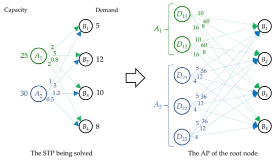
Figure 1.
An illustration of transforming the STP being solved to the AP of the root node.
In Figure 1, A1’s capacity can fulfill the total demand of the two highest-demand destinations (i.e., B2 and B3), and A2’s capacity can fulfill the total demand of the three highest-demand destinations (i.e., B2, B3, and B4). Thus, A1 and A2 own two and three product lots, respectively, in the AP. As the transformation’s result, the AP consists of the five product lots (i.e., D11, D12, D21, D22, and D23) and the four destinations (i.e., B1, B2, B3, and B4). Note that D11 and D12 belong to A1, while D21, D22, and D23 belong to A2. In addition, the assignment costs dikj (which equals bjcij) are given on the arrows pointing from Dik to Bj. An example of calculating dikj is as follows: d213 = b3c23 = 10(1.2) = 12. The AP aims to find the one-to-one assignment of product lots to all destinations that minimizes the total assignment cost.
Every AP’s optimal solution can be interpreted as a solution of the STP being solved as follows: the AP’s optimal solution assigning a specific Dik to a specific Bj is equivalent to the STP’s solution in which Ai ships bj product units to Bj, with the total transportation cost equaling the given total assignment cost. Using the data from Figure 1, Figure 2 illustrates how to interpret the AP’s optimal solution (on the right side) as the solution of the STP being solved (on the left side). Via the Hungarian method, the AP’s optimal solution assigns D11 to B3, D21 to B1, D22 to B2, and D23 to B4 with a total assignment cost of 53. It can be interpreted as the solution of the STP being solved in which A1 ships 10 product units to B3 while A2 ships 5, 12, and 8 product units to B1, B2, and B4, respectively, with a total transportation cost of 53.
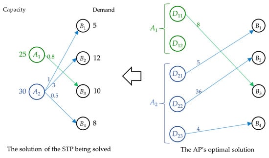
Figure 2.
An illustration of interpreting the AP’s optimal solution as a solution of the STP.
3.2. PH’s Overall Procedure
PH’s overall procedure is presented in Algorithm 2. It uses Algorithm 1 as its component to generate the root node, and it then searches for the optimal solution in the search tree. The notation used in Algorithm 2 is given below:
- Let m denote the number of all sources in the STP.
- Let mi denote the number of all product lots of the source Ai. In the root node, the values of all mi (where i = 1, 2, …, m) are given by Algorithm 1.
- Let l indicate the current level in the search tree.
- The current node means the node, at the current level, selected for branching into m child nodes for the next level.
- The root node is the only node at level 0. It is thus the initial current node, which provides the initial best solution.
- Let Q be the maximum number of candidate child nodes at each level, predetermined by the user. A candidate child node denotes a child node being considered as the new current node.
- Let APcur and Ccur denote the specific AP and its optimal solution’s total assignment cost, respectively, of the current node. Note that the APcur of the root node is taken from Algorithm 1.
- Let APi and Ci denote the specific AP and its optimal solution’s total assignment cost, respectively, of the i-th child node of the current node.
- Let Sbest and Cbest denote the best solution and its total transportation cost, respectively, of the STP found by PH.
- Let LC denote the list of candidate child nodes.
| Algorithm 2. PH’s overall procedure. |
| 1: Receive the STP being solved and the value of Q from the user. 2: Let l = 0. 3: Generate the root node, as the initial current node, by using Steps 3.1 to 3.5. 3.1: Transform the STP to APcur by using Algorithm 1. 3.2: Find the optimal solution of APcur by using the Hungarian method. 3.3: Let Ccur ← the total assignment cost of the optimal solution of APcur. 3.4: Interpret the optimal solution of APcur as a solution of the STP. 3.5: Let Cbest ← Ccur and Sbest ← the STP’s solution taken from Step 3.4. 4: Let l ← l + 1. 5: Generate m child nodes and update Cbest and Sbest by using Steps 5.1 to 5.8. 5.1: Let i ← 1. 5.2: Modify APcur to APi by assigning mi ← mi + 1. After that, for the product lot , let dikj ← bjcij (where k = mi, and j = 1, 2, …, n). 5.3: Find the optimal solution of APi by using the Hungarian method. 5.4: Let Ci ← the total assignment cost of the optimal solution of APi. 5.5: Interpret the optimal solution of APi as a solution of the STP. 5.6: If the STP’s solution taken from Step 5.5 has at least one source suppling more than its capacity, reassign Ci ← +∞, as this STP’s solution is infeasible. 5.7: If Ci < Cbest, update Cbest ← Ci and Sbest ← the STP’s solution taken from Step 5.5. 5.8: If i = m, go to Step 6; otherwise, i ← i + 1 and repeat from Step 5.2. 6: Generate LC by using Steps 6.1 to 6.4. 6.1: Create LC by listing all APi (where i = 1, 2, …, m) sorted in ascending order of Ci. 6.2: Modify LC by keeping only the Q topmost members on the list. 6.3: Modify LC by deleting every member whose Ci is not less than Ccur from the list. 6.4: If LC is empty, go to Step 8; otherwise, go to Step 7. 7: Select the new current node from LC by using Steps 7.1 to 7.3. 7.1: Let APcur ← a member uniform randomly selected from LC. 7.2: Let Ccur ← the total assignment cost of the optimal solution of APcur. 7.3: Repeat from Step 4. 8: Stop the procedure, and return Sbest and Cbest to the user. |
To illustrate how Algorithm 2 works, Figure 3 shows how PH with Q = 5, hereafter called PH-V, searches in a search tree for solving STP01 (which is the first STP instance with 15 sources and 100 destinations described in Section 4). At each level, Figure 3 shows all child nodes with their total transportation costs (given under the nodes) and highlights the current node in yellow; Figure 3 also highlights the node containing the new best solution by coloring its outline green. Because there are 15 sources in STP01, the current node at each level is branched into 15 child nodes for the next level. Note that all the nodes whose total transportation costs are +∞ provide infeasible solutions for the STP.
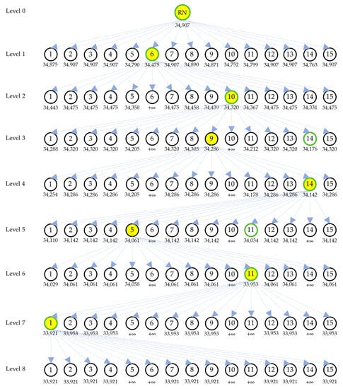
Figure 3.
PH-V’s search in its search tree on a specific run for solving STP01.
In Figure 3, the root node (called RN) at level 0 is the initial current node with a total transportation cost of 34,907. For levels 1 to 7, the current nodes are the sixth child node (with total cost of 34,475), the tenth child node (with total cost of 34,320), the ninth child node (with total cost of 34,286), the fourteenth child node (with total cost of 34,142), the fifth child node (with total cost of 34,061), the eleventh child node (with total cost of 33,953), and the first child node (with total cost of 33,921), respectively. Note that at levels 3 and 5, their new best solutions are not chosen as their current nodes; such cases can occur due to the probabilistic-based selection. Finally, PH-V stops at level 8 because none of the child nodes perform better than the current node. PH-V then returns its last best solution, taken from the first child node at level 7, to the user.
4. Experiment’s Setup
The experiment in this paper was conducted in order to compare performance among the three PH variants (i.e., PH-I, PH-V, and PH-X) and RN on 30 STP benchmark instances. Let PH-I, PH-V, and PH-X denote PHs with Q = 1, Q = 5, and Q = 10, respectively. Let RN denote the second heuristic of [], which is identical to the partial PH having only the root node. In this experiment, RN was chosen as a representative of the existing STP-solving algorithms. The reason for this is that PH is an approximation algorithm and, thus, should be compared in performance with another approximation algorithm, such as RN. Except for RN, most existing STP-solving algorithms [,,,] belong to the class of exact algorithms.
In this paper, a benchmark instance generator was developed for generating the 30 STP benchmark instances, i.e., STP01, STP02, …, STP30. The benchmark instance generator, shown in Algorithm 3, was implemented in C# of Visual Studio 2022. Thus, Algorithm 3 is presented in C# syntax in order to avoid misinterpretation when regenerating these STP benchmark instances in future works. The notation used in Algorithm 3 is defined below:
- Let SEED denote a random seed number for generating a specific STP instance.
- Let NS be the parameter denoting the number of all sources in a specific STP instance with a value of m.
- Let ND be the parameter denoting the number of all destinations in a specific STP instance with a value of n.
- Let CP[i] be the parameter denoting the capacity of the source Ai (where i = 1, 2, …, m) with a value randomly generated in a range [CPMin, CPMax).
- Let DM[j] be the parameter denoting the demand of the destination Bj (where j = 1, 2, …, n) with a value randomly generated in a range [15, 20).
- Let UC[i, j] be the parameter denoting the unit transportation cost from the source Ai to the destination Bj with a value randomly generated in a range [1, 300).
Each STP instance requires a specific value of SEED in Algorithm 3. To generate STP01, STP02, …, and STP30, let SEED in Algorithm 3 be replaced by 1000, 2000, 3000, …, 30,000, respectively. Each STP instance requires not only a specific value of SEED but also specific values of m, n, CPMin, and CPMax in Algorithm 3. To generate each STP instance, let m, n, CPMin, and CPMax in Algorithm 3 be replaced by the values given in Table 1.
| Algorithm 3. Benchmark instance generator. |
| 1: Random rnd = new Random(SEED); 2: int NS = m; 3: int ND = n; 4: int[] CP = new int[NS + 1]; 5: int[] DM = new int[ND + 1]; 6: int[,] UC = new int[NS + 1, ND + 1]; 7: for (int i = 1; i <= NS; i++) 8: { 9: CP[i] = rnd.Next(CPMin, CPMax); 10: } 11: for (int j = 1; j <= ND; j++) 12: { 13: DM[j] = rnd.Next(15, 20); 14: } 15: for (int i = 1; i <= NS; i++) 16: { 17: for (int j = 1; j <= ND; j++) 18: { 19: UC[i, j] = rnd.Next(1, 300); 20: } 21: } |

Table 1.
Parameter values for generating STP instances.
The LB’s value was given for every STP instance, where the LB denotes the lower bound of the optimal solution’s total transportation cost. To compute the LB, let the STP instance be transformed to an AP by using the algorithm modified from Algorithm 1; the modification changes L to be the list of all destinations sorted in ascending order of demand (instead of descending order). Then, the Hungarian method is applied to find the optimal solution of the given AP, and its total assignment cost is used as the value of the LB. This procedure of computing the LB is the same as the procedure of generating the root nodes of A-B and A-S in [].
In the experiment, all the algorithms were coded in C# and executed on an AMD Ryzen 7 4800H processor @ 2.90 GHz with RAM of 8 GB (7.36 GB useable). The Hungarian method used in Algorithm 2 was modified from the source code of [] so that it could then be used with the product lots Dik, which have two indices: i and k. In each instance, PH-V and PH-X were executed for five runs with different random seed numbers, while PH-I and RN were executed for only one run. The reason is that a change in a random seed number may affect PH-V’s and PH-X’s results, but it does not affect those of PH-I and RN.
5. Experiment’s Results and Discussion
This section shows the results and a discussion of the experiment given in Section 4. Table 2 summarizes the experiment’s results, including the final solution values of RN, PH-I, PH-V, and PH-X. Note that, in this section, a solution value means the total transportation cost of a solution of the STP being solved. Table 2 also shows the computational times and the numbers of levels consumed by the algorithms. The notation used in Table 2 is defined as follows:
Table 2.
Experiment’s results.
- In each instance, the LB denotes the lower bound of the optimal solution value.
- RN denotes the second heuristic of [], which is identical to the partial PH that has only the root node. Thus, its solution is equal to the solution given by PH’s root node.
- PH-I, PH-V, and PH-X denote PHs with Q = 1, Q = 5, and Q = 10, respectively.
- For each of RN and PH-I, the columns “Sol” and “Time” present the final solution value (i.e., the last best solution value) and the computational time in seconds, respectively, in each instance. Each of these two algorithms was executed for only one run.
- For only PH-I, the column “No of Levels” presents the number of all used levels, excluding level 0, in each instance.
- For each of PH-V and PH-X, the columns “Best Sol” and “Avg Sol” present the best final solution value and the average final solution value, respectively, over five runs in each instance.
- For each of PH-V and PH-X, the columns “Avg No of Levels” and “Avg Time” present the average number of all used levels (excluding level 0) and the average computational time in seconds, respectively, over five runs in each instance.
According to Table 2, the algorithms PH-I, PH-V, and PH-X obviously outperformed RN in their best and average final solution values. Each PH returned much better final solutions than RN’s final solutions in all 30 instances. Based on the experiment’s results, the binomial tests concluded that each PH tends to win an unknown instance against RN with a p-value of less than 0.001. Remind that RN is not only an existing heuristic [] but also identical to the PH that has only the root node. Thus, the results not only indicated that PHs outperform the existing heuristic [] but also showed that PHs can greatly improve their initial solutions by their tree searching performance.
Unlike the comparison with RN, it is not easy to compare the performance among PH-I, PH-V, and PH-X because they are the same algorithms with different values of Q. However, PH-X seems to be noticeably underperforming in comparison to the two other PHs. Based on the results in Table 2, PH-V outperformed PH-X in both the best and average final solution values. In the best final solution values, PH-V won one instance (i.e., STA10) and drew 29 remaining instances against PH-X. In the average final solution values, PH-V won five instances (i.e., STA10, STA17, STA20, STA27, and STA29), lost one instance (i.e., STA08), and drew 24 remaining instances against PH-X. Based on these five wins and one loss of PH-V against PH-X, a binomial test was conducted for comparing PH-V’s and PH-X’s performance. This test concluded that, given that all instances ending in a draw are excluded, PH-V tends to win an unknown instance against PH-X in the average final solution value with a p-value of 0.109. (Note that an instance ending in a draw means an instance in which the two algorithms return the same result.)
As shown in Table 2, the outperformer between PH-I and PH-V is hard to identify. PH-V performed slightly better than PH-I in the best final solution values but slightly worse in the average final solution values. In the best final solution values, PH-V won one instance (i.e., STA17) and reached a draw in the 29 remaining instances against PH-I. However, in the average final solution values, PH-V won one instance (i.e., STA17), lost three instances (i.e., STA08, STA10, and STA27), and reached a draw in the 26 remaining instances against PH-I. A binomial test was then conducted by using the one win and three losses of PH-V against PH-I. The binomial test concluded that, given that all the instances ending in a draw are excluded, PH-V tends to lose an unknown instance against PH-I in the average final solution value with a p-value of 0.313. Thus, PH-I is recommended if the user decides to use the result taken from only a single run, while PH-V is suggested if the user can wait a longer time for receiving the best result in five or more runs. Another reason is that PH-I is a deterministic algorithm, which always returns the same solution for a specific instance; thus, no benefits can be obtained from executing PH-I multiple runs.
Figure 4 presents the convergence rates of RN, PH-I, PH-V, and PH-X by plotting ADs of the algorithms at each level, where AD denotes the average deviation of the current best solution values from LBs over all runs in all 30 instances. The obstacle of plotting was that each algorithm’s stopping levels are varied according to different instances and random seed numbers. To cope with this obstacle, after the stopping levels, the last best solution values were continuously used in computing AD until level 25. This is the reason that Figure 4 shows the convergence rate of RN, which has only level 0, by the constant from levels 0 to 25. Among the three PHs, the algorithms PH-I, PH-V, and PH-X converged fastest, second fastest, and slowest, respectively. PH-V converged slightly slower than PH-I, while PH-X converged a little slower than the two other algorithms. This comparison result corresponds well to the comparison result in the average final solution values.
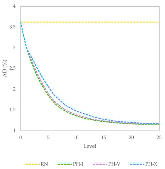
Figure 4.
Convergence rates of RN, PH-I, PH-V, and PH-X.
The findings in this section can be concluded as follows: The PH with a lower Q usually converges faster and, on average, returns a better solution than the PH with a higher Q. This is the reason that PH-I, with Q = 1, performed best in the average final solution values and also converged the fastest. However, Q = 1 turns PH-I into a deterministic algorithm, which always returns the same solution for a particular instance. Thus, the user cannot obtain any better solution from executing PH-I multiple runs. When Q’s value is set higher, PH’s ability is enhanced in searching along the branches that may not contain the best nodes at their levels. Thus, the PH with a higher Q has a higher potential to avoid getting stuck into the same solution for different runs. This is the reason that, with Q = 5, PH-V performed slightly better than PH-I in the best final solution values. However, if Q’s value is set too high, PH may lose the opportunity to find optimal or near-optimal solutions. Based on the experiment’s results, Q = 10 is defined too high and should be avoided because PH-X performed the worst among the three PHs in terms of both the final solution value and convergence rate. Thus, PH-I is recommended if the user decides to take the result from a single run, while PH-V is suggested if the user decides to wait a longer time to receive the best result from five or more runs.
6. Conclusions
PH is the probabilistic hill-climbing tree search algorithm for the STP. In PH’s search tree, each node contains an AP transformed from the STP being solved. The transformation is performed by converting each source’s product units to product lots, in which a product lot equals multiple product units; each AP aims to assign a product lot to every destination. The difference among the APs of all nodes is the number of each source’s product lots. In the AP of the root node (as the initial current node), the number of each source’s product lots is set to be small enough to avoid the capacity insufficiency in the STP. To generate every subsequent level, PH branches from the current node into m child nodes, where m is the number of all sources in the STP. The AP of the i-th child node is modified from the AP of the current node by adding one more product lot into the i-th source, where i = 1, 2, …, m. Then, PH moves to the new current node, which is randomly selected from Q candidate child nodes. In the experiment, the performance of the three PHs (i.e., PH-I, PH-V, and PH-X) and RN was compared. All the PHs performed much better than RN, and PH-X performed a little worse than the two other PHs. PH-V performed slightly better than PH-I in the best final solution values but slightly worse in the average final solution values. Future works should focus on both improving the STP model for real-world applications and enhancing PH’s performance.
Funding
This research received no external funding.
Institutional Review Board Statement
Not applicable.
Informed Consent Statement
Not applicable.
Data Availability Statement
All the material conducted in the study is mentioned in article.
Conflicts of Interest
The author declares no conflict of interest.
References
- Reeb, J.; Leavengood, S. Transportation Problem: A Special Case for Linear Programming Problems. In Technical Report EM 8779; Oregon State University: Corvallis, OR, USA, 2002. [Google Scholar]
- Pentico, D.W. Assignment problems: A golden anniversary survey. Eur. J. Oper. Res. 2007, 176, 774–793. [Google Scholar] [CrossRef]
- De Maio, A.; Roveda, C. An all zero-one algorithm for a certain class of transportation problems. Oper. Res. 1971, 19, 1406–1418. [Google Scholar] [CrossRef]
- Srinivasan, V.; Thompson, G.L. An algorithm for assigning uses to sources in a special class of transportation problems. Oper. Res. 1973, 21, 284–295. [Google Scholar] [CrossRef]
- Nagelhout, R.V.; Thompson, G.L. A single source transportation algorithm. Comput. Oper. Res. 1980, 7, 185–198. [Google Scholar] [CrossRef]
- Pongchairerks, P. An integration between assignment and transportation models. J. Res. Eng. Technol. 2005, 2, 377–390. [Google Scholar]
- Pongchairerks, P. Efficient heuristics for single-source transportation problems. Int. J. Appl. Phys. Math. 2014, 4, 352–362. [Google Scholar] [CrossRef]
- Geunes, J. Operations Planning: Mixed Integer Optimization Models; CRC Press: Boca Raton, FL, USA, 2015. [Google Scholar]
- Nauss, R.M. Solving the generalized assignment problem: An optimizing and heuristic approach. INFORMS J. Comput. 2003, 15, 249–266. [Google Scholar] [CrossRef]
- Munapo, E.; Tawanda, T.; Nyamugure, P.; Kumar, S. Solving the GAP by cutting its relaxed problem. In Lecture Notes in Networks and Systems; Springer: Cham, Switzerland, 2023; Volume 569, pp. 832–842. [Google Scholar]
- Zhi-Bin, H.; Guang-Tao, F.; Dan-Yang, D.; Chen, X.; Zhe-Lun, D.; Zhi-Tao, D. Novel parallel hybrid genetic algorithms on the GPU for the generalized assignment problem. J. Supercomput. 2022, 78, 144–167. [Google Scholar] [CrossRef]
- Dörterler, M. A new genetic algorithm with agent-based crossover for the generalized assignment problem. Inf. Technol. Control. 2019, 48, 389–400. [Google Scholar] [CrossRef]
- Pongchairerks, P. An enhanced two-level metaheuristic algorithm with adaptive hybrid neighborhood structures for the job-shop scheduling problem. Complexity 2020, 2020, 3489209. [Google Scholar] [CrossRef]
- Pongchairerks, P. A job-shop scheduling problem with bidirectional circular precedence constraints. Complexity 2021, 2021, 3237342. [Google Scholar] [CrossRef]
- Pongchairerks, P. A two-level metaheuristic for the job-shop scheduling problem with multipurpose machines. Complexity 2022, 2022, 3487355. [Google Scholar] [CrossRef]
- Taylor, B.W. Introduction to Management Science, 13th ed.; Pearson: Boston, MA, USA, 2019. [Google Scholar]
- Raphael, B.; Smith, I.F.C. Engineering Informatics: Fundamentals of Computer-Aided Engineering, 2nd ed.; Wiley: West Sussex, UK, 2013. [Google Scholar]
- Araya, I.; Riff, M.-C. A beam search approach to the container loading problem. Comput. Oper. Res. 2014, 43, 100–107. [Google Scholar] [CrossRef]
- Sabuncuoglu, I.; Bayiz, M. Job shop scheduling with beam search. Eur. J. Oper. Res. 1999, 118, 390–412. [Google Scholar] [CrossRef]
- Tyugu, E. Algorithms and Architectures of Artificial Intelligence; IOS Press: Amsterdam, The Netherlands, 2007. [Google Scholar]
- Koller, D.; Friedman, N. Probabilistic Graphical Models: Principles and Techniques; MIT Press: Cambridge, MA, USA, 2009. [Google Scholar]
- Bennell, J.A.; Song, X. A beam search implementation for the irregular shape packing problem. J. Heuristics 2010, 16, 167–188. [Google Scholar] [CrossRef]
- Blum, C.; Blesa, M.J. Probabilistic beam search for the longest common subsequence problem. In Lecture Notes in Computer Science; Springer: Berlin/Heidelberg, Germany, 2007; Volume 4638, pp. 150–161. [Google Scholar]
- Wang, F.; Lim, A. A stochastic beam search for the berth allocation problem. Decis. Support Syst. 2007, 42, 2186–2196. [Google Scholar] [CrossRef]
- Basseur, M.; Goëffon, A. Hill-climbing strategies on various landscapes: An empirical comparison. In Proceedings of the 15th Annual Conference on Genetic and Evolutionary Computation, Amsterdam, The Netherlands, 6–10 July 2013; pp. 479–486. [Google Scholar]
- Charnsethikul, P. An Exact Branch and Bound Algorithm for the General Quadratic Assignment Problem. Ph.D. Thesis, Texas Tech University, Lubbock, TX, USA, 1988. [Google Scholar]
- Regueiro, A. Hungarian Algorithm. Available online: https://web.archive.org/web/20121106104729/http://noldorin.com:80/programming/HungarianAlgorithm.cs (accessed on 23 January 2020).
Disclaimer/Publisher’s Note: The statements, opinions and data contained in all publications are solely those of the individual author(s) and contributor(s) and not of MDPI and/or the editor(s). MDPI and/or the editor(s) disclaim responsibility for any injury to people or property resulting from any ideas, methods, instructions or products referred to in the content. |
© 2023 by the author. Licensee MDPI, Basel, Switzerland. This article is an open access article distributed under the terms and conditions of the Creative Commons Attribution (CC BY) license (https://creativecommons.org/licenses/by/4.0/).