Article

Water Pollution and Pollution–Control Capacity in Chinese Provinces: Panel Estimations of Provincial Environmental Kuznets Curves

1
Graduate School of Humanities and Social Sciences, Saitama University, Saitama 338-8570, Japan
2
Graduate School of Science and Engineering, Saitama University, Saitama 338-8570, Japan
*
Author to whom correspondence should be addressed.
Sustainability 2023, 15(5), 3979; https://doi.org/10.3390/su15053979
Submission received: 14 December 2022 / Revised: 19 February 2023 / Accepted: 20 February 2023 / Published: 22 February 2023

Abstract

:
China’s rapid industrialization and urbanization in recent decades have deteriorated its water resource quality. This study focused on water pollution in terms of the chemical oxygen demand (COD) and the levels of ammonia nitrogen in the industrial and household discharges of different Chinese provinces. Although the heterogeneity of environmental Kuznets curves (EKCs) from Chinese provinces has been studied, the positions of provincial EKCs (which reflect the province-specific pollution effects not affected by the provincial income levels) have not been investigated to date. Therefore, through a factor analysis of the heterogeneity of provincial pollution under the EKC framework, we investigated how the capacity shortage for pollution control contributes to the provincial pollution levels. We also evaluated the heterogeneity of the EKCs from the provinces in terms of their positions (not their shapes), using a fixed-effect model to extract the province-specific pollution effects. The capacity shortage for pollution control, as one of the pollution factors, accounted for (a) 30% of industrial COD and industrial ammonia nitrogen; (b) 60% of household COD; and (c) 80% of household ammonia nitrogen. Our results indicate that China still has a large capacity to mitigate water pollution via policies and by building the capacity for pollution control through the development and training of human resources.

1. Introduction

China’s growth has significantly improved the country’s living standards since the implementation of the Open-door policy and the Reform Policy in 1978. The economic status of China was promoted from the low-income category to the lower-middle-income category in 1997, and to upper-middle-income category in 2010, based on the World Bank income classification. However, this rapid economic development resulted in serious damages to its environment through industrialization and urbanization. Water pollution is one of the vital issues that influences the survival of human beings and the development of socio-economic systems. According to the Environmental Performance Index, China remains in 80th place among 180 countries in terms of water resources. To address the issue of water pollution, the Chinese government has set numerical targets to reduce the two main water pollutants: chemical oxygen demand (COD) discharge, after the 11th Five-Year Plan (2006–2010), and ammonia nitrogen discharge, after the 12th Five-Year Plan (2011–2015). The current 14th Five-Year Plan (2021–2025) contains binding targets to reduce COD and ammonia nitrogen discharges by 8% during the planned period. These targets have been almost achieved through policy efforts; however, the pollution discharges still remain massive, keeping the water quality at a low level. The groundwater supplies in more than half of the Chinese cities were categorized as “bad to very bad,” while more than a quarter of China’s major rivers were considered “unfit for human contact” in 2014 [1,2]. In addition to the nation-wide issue of water pollution, another vital concern in China is the regional heterogeneity of the pollution levels and the factors influencing them. The water pollution levels largely differ by provinces, and the industrialization, urbanization and pollution-control capacities that affect pollution levels vary by provinces. There are also policy priority areas for water pollution control that have been set by the Chinese government [3]. (COD and ammonia nitrogen originate from the same sources, and the major industries that emit these pollutants are papermaking, textile and chemical ones (Cai et al. [1], Liu et al. [4]). China’s sewage treatment mainly adopts six major sewage treatment processes: the oxidation ditch process, the A2/O process, the traditional active sewage treatment method, the SBR process, the A/O process, and the biofilm process (Ministry of Ecology and Environment of China [5]).
This study focused on the water pollution measures that target COD and ammonia nitrogen from industrial and household discharges in Chinese provinces, and aimed to investigate the contribution of capacity shortage to the pollution control of provincial pollution levels, through a factor analysis that evaluated the heterogeneity of provincial pollution under the analytical framework of the environmental Kuznets curve (EKC). We performed the following steps: (1) the EKC was estimated econometrically from the provincial panel data using a fixed-effect model; (2) the province-specific pollution effect was extracted from the fixed effect, which is not affected by the provincial income level, on the EKC; (3) the alternative EKC was re-estimated by replacing the fixed-effect model with the possible contributors to the province-specific pollution, such as the capacity for pollution control, the industrialization degree (for industrial discharges), and the urbanization degree (for household discharges); and (4) the contribution of the capacity shortage to the pollution control of the province-specific pollution level was quantified through a factor analysis.
The main finding of this study is that the capacity shortage for pollution control, as one of the pollution factors, accounts for (a) about 30% of industrial COD and industrial ammonia nitrogen; (b) about 60% of household COD; and (c) about 80% of household ammonia nitrogen. Therefore, China still has much capacity to mitigate COD-related species and ammonia nitrogen via policy change.
The remainder of the paper is structured as follows. Section 2 reviews the literature related to the EKC issues, including water pollution in China, and clarifies this study’s contributions. Section 3 shows the materials and methods for the empirical study. Section 4 presents the estimation results and the discussion. Section 5 summarizes and concludes this paper.

2. Literature Review and Contributions

The EKC provides an analytical framework to examine how economies deal with environmental issues. It postulates an inverted-U-shaped relationship between pollution and economic development. Kuznets’s name was apparently attached to the curve by Grossman and Krueger [6], who noted its resemblance to Kuznets’ inverted-U relationship between income inequality and development. The EKC dynamic process is defined as follows. In the first stage of industrialization, pollution worsens rapidly because people are more interested in jobs and income than in clean air and water, and environmental regulation is correspondingly weak. Along the curve, pollution reduces in wealthy societies, because leading industrial sectors become cleaner, people value the environment, and regulatory institutions become more effective [7].
Since the report of the World Bank [8] initially discussed EKC issues, empirical tests and theoretical debates have intensified, supporting the applicability of EKC for some regions and environment problems [9,10,11,12]. At the initial stage until the 1990s, most of the empirical studies focused on validating the EKC hypothesis and its requirements using cross-sectional data. Since the late 1990s, however, the EKC studies have shifted from cross-sectional analyses to time-series analyses, and more importantly, have examined the heterogeneity of EKCs from individual economies, in terms of the curve’s shapes and positions. In this context, Dasgupta et al. [7] presented three different EKC scenarios from the conventional inverted-U EKC: Race to the Bottom (pessimistic, with a continuation of the highest level of pollution), New Toxics (pessimistic with a higher curve, owing to the newly emerging pollutants), and Revised EKC (optimistic with a lower and flatter curve, owing to a better management of pollution). These scenarios have been subjected to empirical tests [13,14,15,16]. Sarkodie and Strezov [17] comprehensively reviewed the heterogeneity of the EKC modalities in terms of the curve’s shapes and positions.
There is a large body of literature on EKC studies for several countries and for several levels of environmental quality; however, studies on the EKC of China have increased since the 2000s. Therefore, there is a relatively limited number of EKC studies, particularly on water pollution in China, that cover total provinces or specific areas (Table 1). Their estimations show ambiguous and mixed outcomes; some studies identify the validity of the inverted-U-shaped EKC [2,18,19,20,21], whereas the others demonstrate that the EKC modality is dependent on regions and pollutants [1,4,22,23,24].
With respect to the heterogeneity of EKCs from Chinese provinces, Cai et al. [1] demonstrated the varying types of EKCs depending on the province: “good EKCs” (negative monotonic shape, inverted N-shape, inverted U-shape, and M-shape), “bad EKCs” (positive monotonic shape, N-shape, and U-shape), and “transition EKCs” (positive monotonic and flat-tailed shape). To the best of our knowledge, there are no studies investigating the “positions” of provincial EKCs and that reflect the province-specific pollution effects that are not affected by the provincial income levels. Therefore, this study focused on analyzing the heterogeneity of EKCs from different Chinese provinces in terms of their positions using a fixed-effect model in the EKC panel estimation, in order to extract the province-specific pollution effects, and to elucidate the factors influencing the province-specific pollution levels. This study focused particularly on the provincial capacity for controlling the pollution levels.

3. Materials and Methods

3.1. Methodology and Data

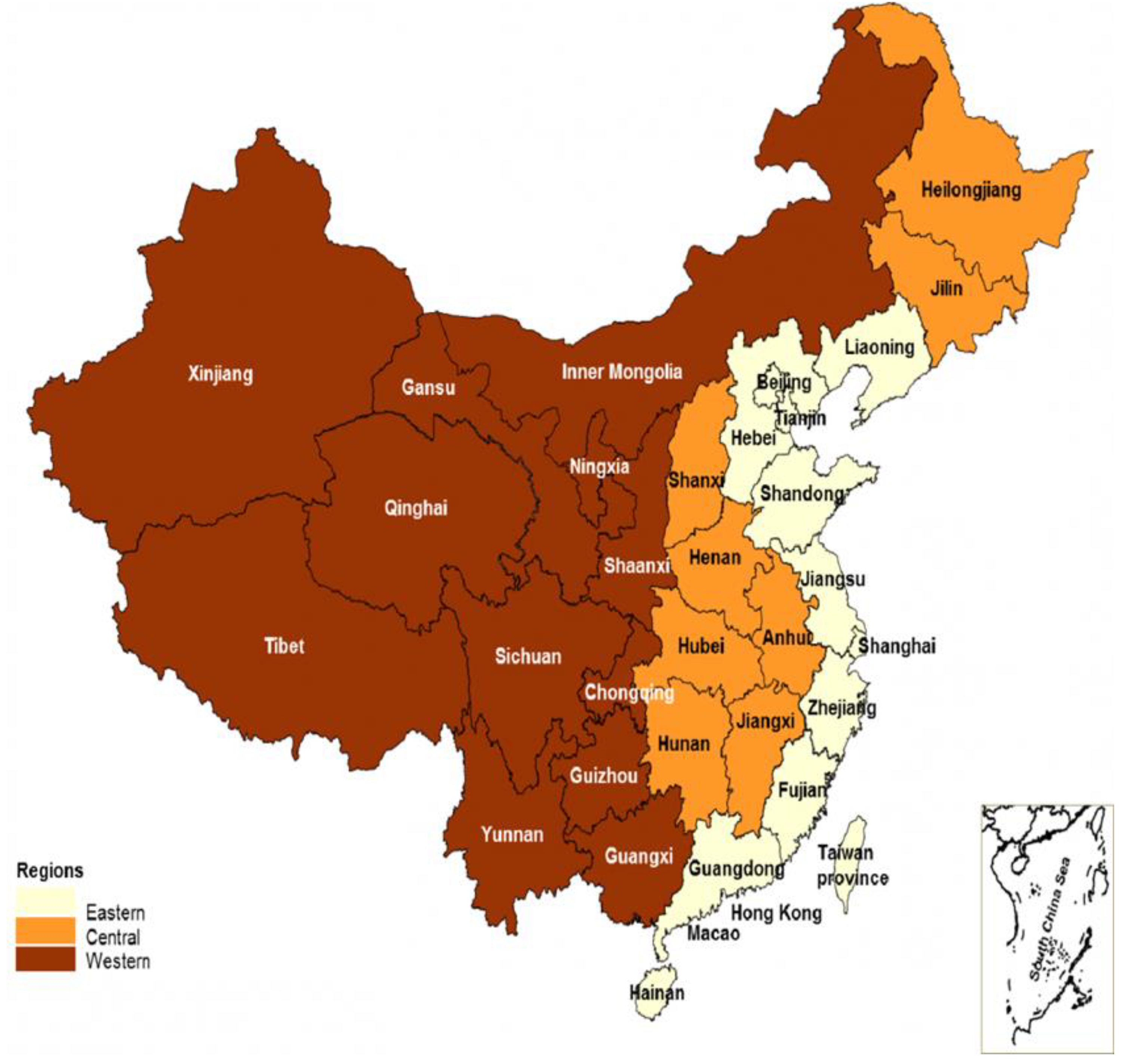
This section first overviews the heterogeneity of Chinese provinces in terms of their water pollution levels and the factors influencing them (Table 2, as for the location see Appendix A). According to the China Statistical Yearbook, in 2020, the industrial discharge of COD per million persons varied from 65 tons in Beijing to 700 tons in Jiangsu; the household discharge of COD was from 1848 tons in Beijing to 11,488 tons in Guangxi; the industrial discharge of ammonia nitrogen was from 2 tons in Beijing to 36 tons in Jiangxi; and the household discharge of ammonia nitrogen was from 94 tons in Tianjin to 1149 tons in Guangxi. The economic factors influencing pollution should be considered; the gross regional product (GRP) per capita in 2010 differed from 127,816 yuan in Beijing to 28,171 yuan in Gansu; the secondary industry’s value added as a percentage of GRP (affecting industrial discharges) differed from 46.2% in Fujian to 16.0% in Beijing; and the urban population as a percentage of the total population (affecting household discharges) differed from 89.3% in Shanghai to 35.8% in Tibet. In addition, there are policy priority areas that are designated as key regions for water pollution control by the Chinese government and that are imposed with several regulations to improve water quality. This includes three river (Huai, Hai, and Liao) and three lake (Tai, Chao, and Dianchi) basins (hereafter, 3Rs3Ls) that are spread across 11 provinces (last column of Table 1 [3]). The authors identified the 11 provinces based on Wang et al. [3].
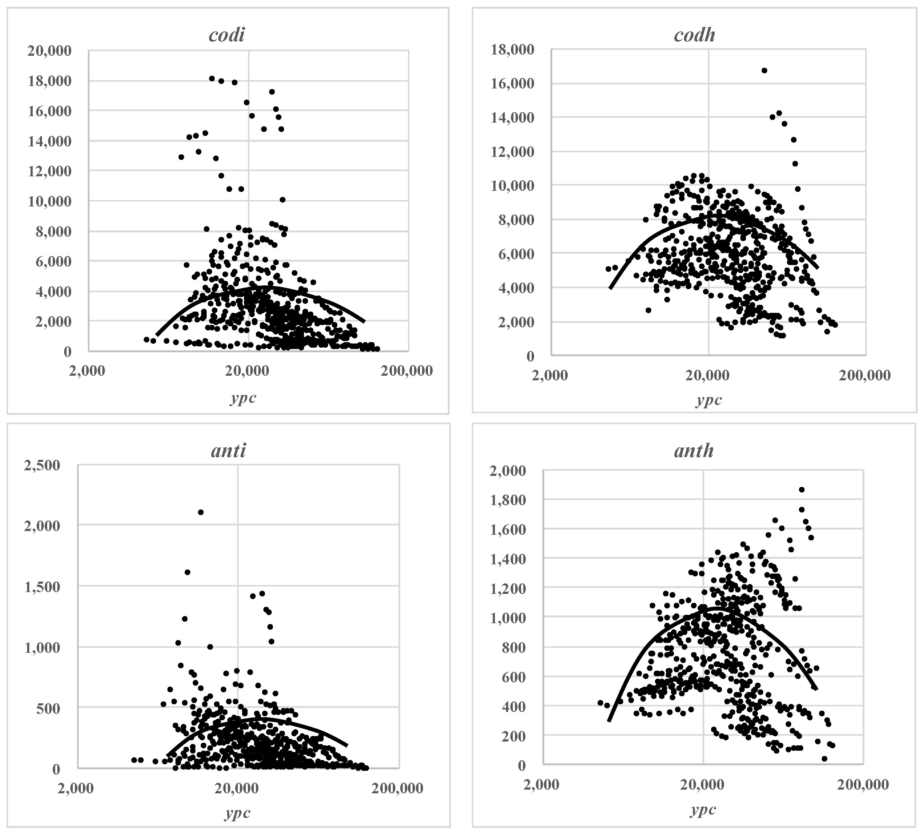
This study follows the original form of the EKC: the standard nonlinear model in which water pollution per capita is regressed by income per capita and its square. The original EKC postulates an inverted-U-shaped nexus between pollution per capita and income per capita. Figure 1 depicts the relationships between the water pollution indicators (vertical axis) and the GRP per capita (horizontal axis) in the total 31 sampled Chinese provinces and periods for 2003−2019; they roughly appear to be inverted-U-shaped. The patterns should be further examined by the subsequent econometric tests by controlling the other factors affecting pollution.
We now turn to econometric approaches. The first specification in Equation (1) applies a fixed-effect model for provincial panel-data estimation in order to explicitly demonstrate the province-specific pollution effects and also run the alternative models in Equations (2) and (3) by replacing the fixed effects with the possible pollution contributors (pollution-control capacity, industrialization, and urbanization) to the province-specific pollution effects. The equations for the estimation are as follows:
ln (codiit, codhit, antiit, anthit) = α0 + α1 ln ypcit + α2 (ln ypcit)2 + fi + ft + εt
ln (codiit, antiit) = β0 + β1 ln ypcit + β2 (ln ypcit)2 + β3 eduit + β4 indit + ft + εt
ln (codhit, anthit) = γ0 + γ1 ln ypcit + γ2 (ln ypcit)2 + γ3 eduit + γ4 urbit + ft + εt
where the subscript it denotes the 31 sampled Chinese provinces for the years 2003−2019, respectively; codi, codh, anti, and anth represent the water pollutants: industrial COD, household COD, industrial ammonia nitrogen, and household ammonia nitrogen, respectively, expressed as tons per million persons; ypc shows the gross regional product (GRP) per capita in yuan at constant prices in 2010; edu denotes the number of higher education graduates per million persons; ind shows the secondary industry value added as a percentage of GRP; urb represents the urban population as a percentage of the total population; fi and ft show a time-invariant country-specific fixed effect and a country-invariant time-specific fixed effect, respectively; ε denotes a residual error term; α0…2, β0…4, and γ0…4 represent estimated coefficients; and ln shows a logarithm form, which is set to avoid scaling issues for the water pollutants and GRP per capita. The data source of all the variables is the China Statistical Yearbook. The study constructs a set of panel data for the 31 sample provinces for the period 2003−2019. (This study excluded the year 2020 when the COVID-19 pandemic seriously affected economic activities). The list and descriptive statistics for the variable data are displayed in Table 3 and Table 4, respectively.
The notes on the specifications of the estimation models in (1), (2), and (3) are required for an additional description as follows. Equation (1) applies a fixed-effect model, represented by fi and ft, for provincial panel-data estimation. The Hausman test is generally used for choosing between a fixed-effect model and a random effect model [
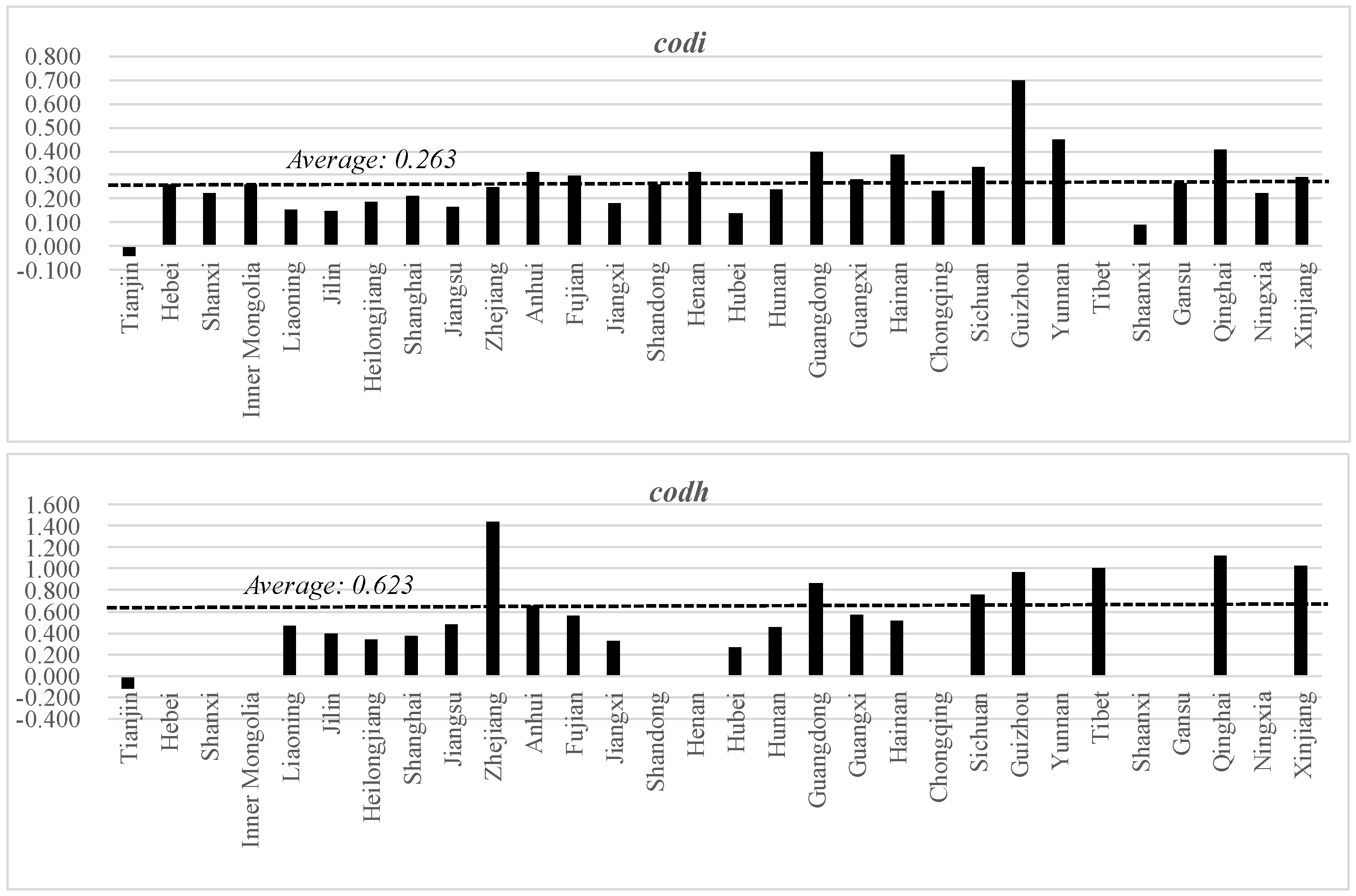
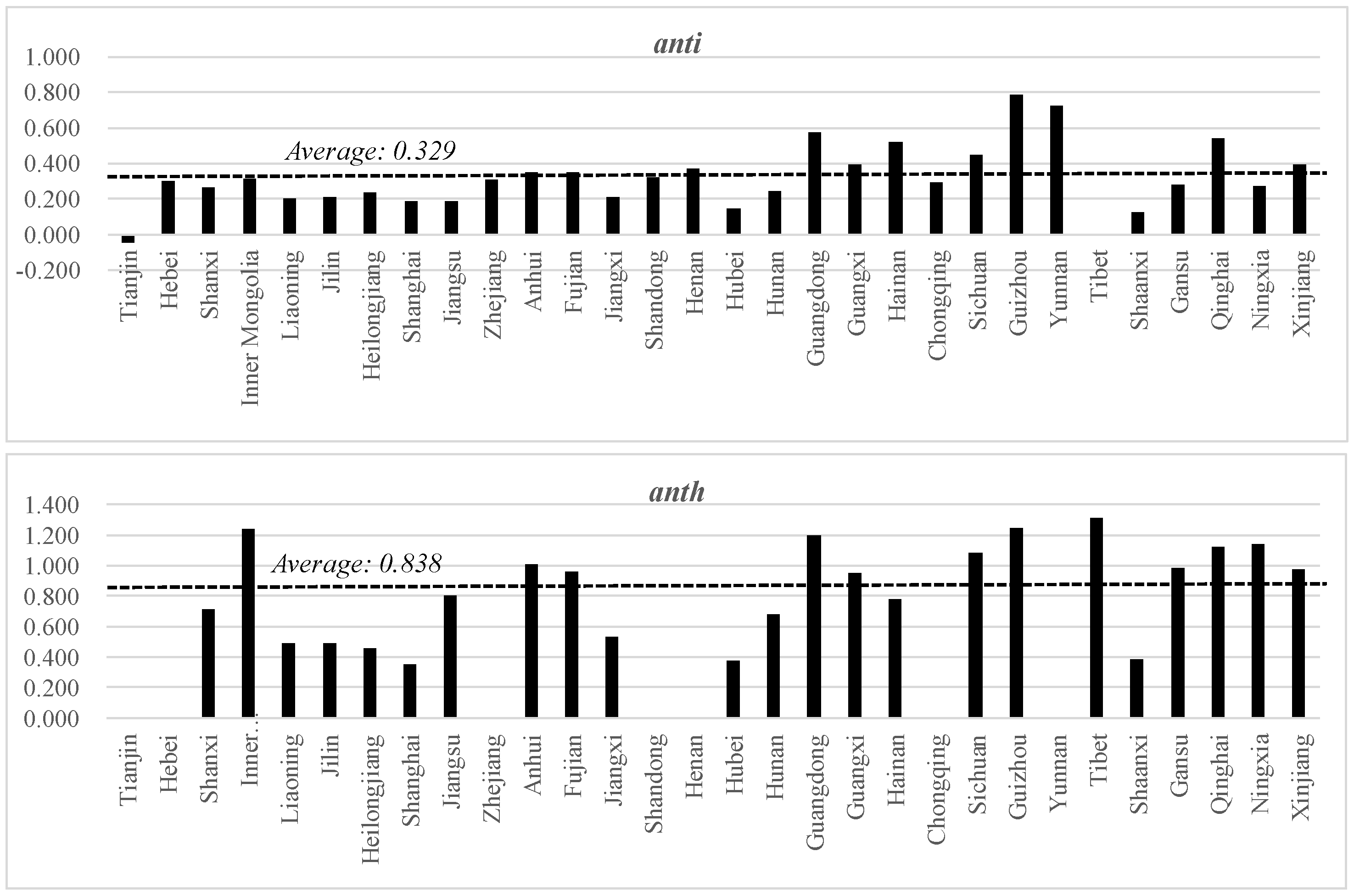
25]. This study, however, focused on demonstrating province-specific pollution effects explicitly; time-specific factors such as economic fluctuations due to external shocks, such as the Asian financial crises in 1997–1998 and the global financial crises in 2008–2009, were considered. In addition, adopting the fixed-effect model contributes to alleviating the endogeneity problem by absorbing the unobserved time-invariant heterogeneity among the sample provinces. The estimation sets Beijing as the benchmark province for extracting the province-specific pollution effects, because Beijing shows the best performance in water pollution control (Table 1). The significantly positive coefficient of the province-specific fixed effect suggests that the water pollution in the particular province is more serious than that in Beijing. The ordinary hypothesis of the EKC postulating the inverted-U-shaped path between water pollution and GRP per capita would be verified if α1, β1, γ1 > 0 and α2, β2, γ2 < 0 are significant with reasonable levels of turning points.
Equations (2) and (3) represent the alternative models for industrial discharges and household discharges, respectively. Equation (2) replaces the province-specific fixed effects with the possible pollution contributors of the fixed effects: pollution-control capacity (edu) and industrialization (ind). Equation (3) replaces them with pollution-control capacity (edu) and urbanization (urb). This study uses the number of graduates of higher education (edu) to represent the capacity to control pollution because the pollution controllability depends highly on human resources and capital in order to address the pollution level in each province. We attempted to apply the variable of treatment plant capacity as the capacity to control pollution. Appendix B showed that the daily treatment capacity of sewage (tcs) was positively correlated with water pollution. It suggests that the treatment plant capacities have only chased after the pollution and thus are equipped with no significant power for pollution control. The importance of human capital in controlling environmental pollution has been studied widely [26,27,28]. The adoption of industrialization (ind) and urbanization (urb) is based on Liu et al.’s study [22]; secondary industry output can be a main indicator for industrial water use, and urban population can be an indicator for household water use. We considered the adoption of the indicators directly measuring industrial and household waste water discharge rates. However, these data are available only for 2003–2015 (the Government has stopped publishing these data since 2016). Another problem is that the level of waste water discharge itself can be affected by pollution control variables, which leads to a multicollinearity problem. Thus, this study alternatively used the indirect indicators, including industrialization and urbanization. Appendix C attempted the estimation using the direct indicators and still found negative coefficients for the pollution control variable (edu), despite some instabilities in the coefficients due to the problems above. No multicollinearity problem exists in the regressors’ combinations in Equations (2) and (3), namely, (ypc, edu, ind) and (ypc, edu, urb). This is because the variance inflation factors (VIFs), reflecting the level of collinearity between the regressors, indicate lower values than the criteria of collinearity (10 points) in each equation. The VIF values of ypc, edu, and ind in Equation (2) are 2.793, 2.765, and 1.017, respectively, and those of ypc, edu, and urb in Equation (3) are 5.417, 2.737, and 4.111, respectively, according to the authors’ estimation. The pollution-control capacity (edu) is expected to impart a negative coefficient for water pollution because the higher capacity enables the mitigation of pollution. The coefficients of industrialization (ind) and urbanization (urb), which deteriorate water quality, are supposed to be positive in the respective equations.
The explanatory variables in Equations (1)–(3), ypc, ind, and urb were lagged by one year. This helps avoid reverse causality in the model specifications, including the endogenous interaction between the dependent and independent variables. For the pollution-control capacity (edu), a 10-year lag was applied because it takes a long time for graduates of higher education to be trained for capacity building for pollution control. 
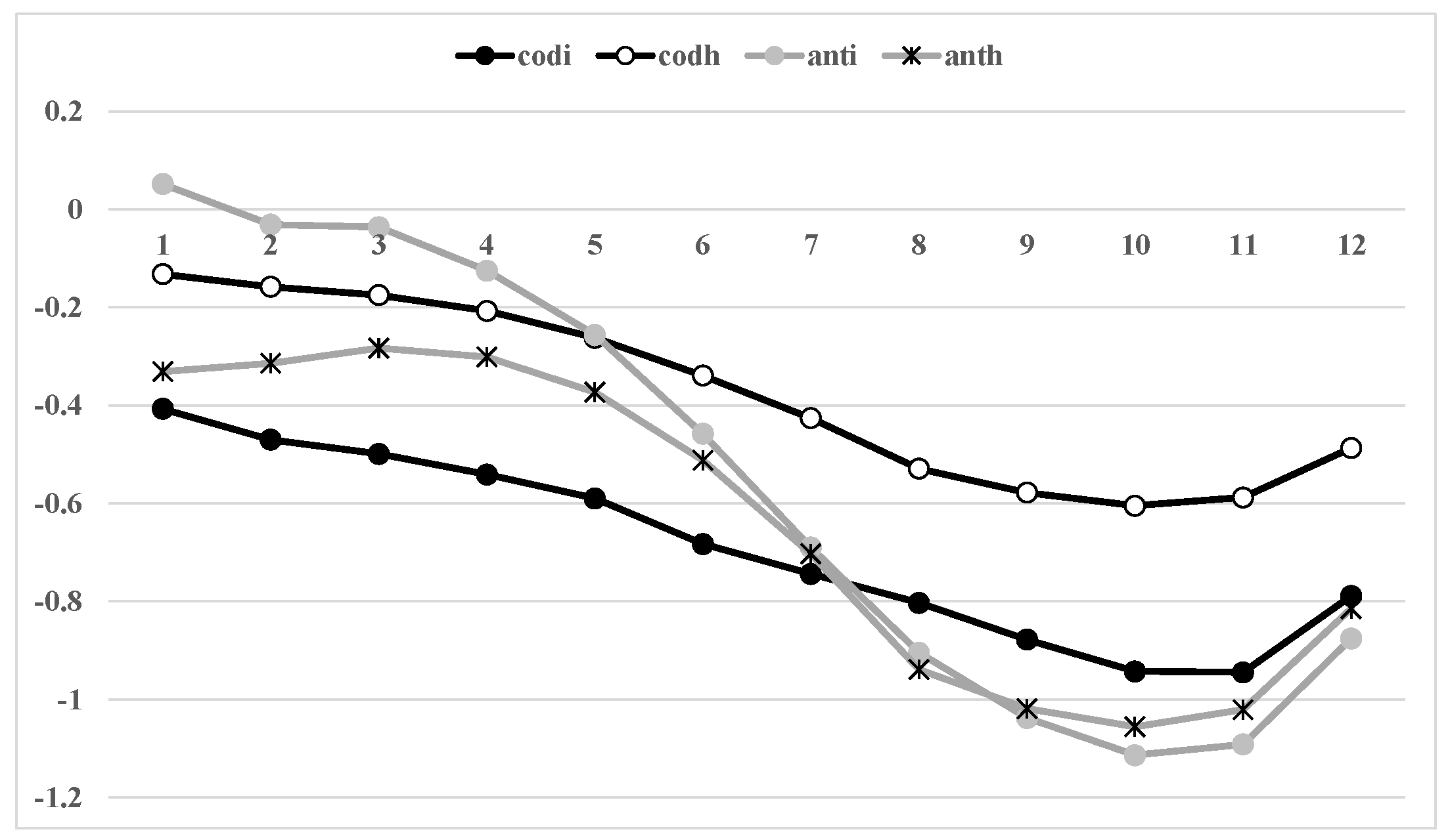
Figure 2 displays the magnitudes of negative coefficients for the pollution-control capacity (edu) using time series lag patterns from Equations (2) and (3), estimated for each water pollutant; the impacts of the capacity on pollution levels are negatively maximized around the 10-year lag, though the impact sizes differ according to the difference in the effects by their treatment processes.
This study applies the ordinary least squares (OLS) estimator and the Poisson pseudo-maximum likelihood (PPML) estimator for the estimations. The PPML estimator was selected because the sample data with heterogeneity in the provincial properties would be plagued by heteroskedasticity and autocorrelation; in such cases, the OLS estimator leads to bias and inconsistency in the estimates. The PPML estimator corrects for heteroscedastic error structure across panels and autocorrelation with panels, as Silva and Tenreyro [29] and Kareem et al. [30] suggest. Therefore, these two estimators are applied to ensure the robustness of the estimations. We used EViews (version 12) (IHS Global Inc., CA, USA) for processing the data and estimations.

3.2. Panel Unit Root and Cointegration Tests

For the subsequent estimation, we investigated the stationary property of the panel data by utilizing panel unit root tests, and if necessary, a panel cointegration test for a set of variables’ data. The panel unit root tests were first conducted on the null hypothesis such that a level and/or the first difference of the individual data have a unit root. In cases where the unit root tests reveal that each variable’s data are not stationary in the level, but stationary in the first difference, a set of variables’ data correspond to the case of I(1); this can be further examined using a co-integration test for the “level” data. If a set of variables’ data are identified to have a co-integration, the use of the “level” data is justified for model estimation.
For the panel unit root tests, this study applied the Levin, Lin, and Chu test [31] as a common unit root test, and the Fisher-ADF and Fisher-PP tests [32,33] as individual unit root tests. The common unit root test assumes a common unit root process across cross-sections, and the individual unit root test allows for individual unit root processes that vary across cross sections. For a panel co-integration test, the study used the Pedroni residual co-integration test (developed by Pedroni [34]). All of the test equations contained an individual intercept and trend, with the lag length being an automatic selection.
Table 5 presents the test results: the common unit root test rejects the null hypothesis of a unit root at the conventional significance levels for all of the variables. However, the individual tests do not reject a unit root in their levels, except edu, while rejecting it in their first differences; therefore, the variables almost follow the case of I(1). The panel co-integration test was conducted further on the combinations of variables in Equations (2) and (3). The panel PP and ADF tests suggested that the level series of a set of variables’ data are co-integrated in the respective combinations. Thus, this study utilizes the level data for the estimation.

4. Results and Discussion

Table 6, Table 7, Table 8 and Table 9 present the results of the OLS and PPML estimations in the form of a log-link function for industrial and household COD, and industrial and household ammonia nitrogen, respectively. Columns (i) and (ii) display the outcomes of the fixed-effect models, and columns (iii) and (iv) present the results of the alternative models containing pollution-control capacity (edu) and industrialization (ind) for industrial discharges, and pollution-control capacity (edu) and urbanization (urb) for household discharges, instead of the fixed effects. Both the OLS and PPML estimations show similar results in the sign and significance of each coefficient; therefore, the subsequent description focuses on the result of the PPML estimations that adjust heteroskedasticity and autocorrelation. The findings from the estimation results are summarized as follows.

4.1. EKC Identification by Fixed-Effect Model

First, the EKC hypothesis, which assumes the inverted-U-shaped relationship between water pollution level and GRP per capita, was confirmed in all the water pollutants from Table 6, Table 7, Table 8 and Table 9 and in all the estimations from columns (i)–(iv). They were confirmed using the estimation results; the coefficients of the GRP per capita were significantly positive, and those of its square were significantly negative. The turning points fell within the reasonable ranges of GRP per capita between its minimum and maximum levels in the samples shown in Table 4, except for the estimations in columns (i) and (ii) in Table 6 (the turning point was computed using –α1/2α2, –β1/2β2, or –γ1/2γ2 in the Equations (1)–(3)). The finding of the inverted-U-shaped EKC in Chinese provinces in this study is consistent with previous studies: Zhang et al. [2], Zhao et al. [18], Li et al. [19], Jayanthakumaran and Liu [20], and Shen [21] in Table 2. The main research focus in this study was, however, the provincial EKC positions rather than their shapes, as in the subsequent description.

4.2. Extraction of Provincial-Specific Pollution Effect

Second, the fixed-effect models in columns (i) and (ii) identified the positive coefficients as the province-specific fixed effects at conventional significant levels, in all the provinces for industrial COD in Table 6 and for household ammonia nitrogen in Table 9, and in the majority of provinces for household COD (except Hebei, Shandong, Henan, Chongqing, and Ningxia) in Table 7 and for industrial ammonia nitrogen (except Tibet) in Table 8. The positive provincial fixed effects mean that the provincial EKCs are located above Beijing, which is the benchmark, suggesting that the province-specific pollution effects (not affected by the provincial income level on the EKC) are larger than those in Beijing. These results are in line with the simple observations on water pollution per capita in all the provinces in Table 1. The degree of water pollution was indicated by the magnitude of the coefficients of provincial fixed effects: the industrial COD in Tianjin via the PPML estimation (column (ii) in Table 6), for instance, was exp. (1.825) = 6.203 times larger than that in Beijing. The provincial fixed effects also revealed that the pollution levels in the policy propriety areas (3Rs3Ls), shown in Table 1, were not necessarily higher than the average levels among the 31 provinces for all water pollutants, thereby implying that the government policies have controlled the water pollution in the priority areas.

4.3. Re-Estimation Results of Alternative EKC Model

Third, in the alternative model containing pollution-control capacity (edu) and industrialization (ind)/urbanization (urb) in columns (iii) and (iv), respectively, the coefficients of edu were significantly negative in all the pollutants and estimations in Table 6, Table 7, Table 8 and Table 9; those of ind for industrial discharges in Table 6 and Table 8 and those of urb for household discharges in Table 7 and Table 9 were significantly positive in all estimations. These results are in line with the hypothesis of Liu et al. [22], stating that the secondary industry output and urban population can be the main indicators of industrial and household water use, respectively. More importantly, the negative coefficients of edu for all pollutants suggest that the pollution-control capacity had, indeed, affected the provincial pollution levels and that the heterogeneity of provincial pollution could be explained by the differences in the provincial pollution-control capacity. The joint estimation outcomes of the province-specific pollution effects and the workability of pollution-control capacity lead to a question regarding the quantitative contributions of provincial capacity shortage to pollution control at the provincial pollution level.

4.4. Factor Analysis on Pollution-Control Capacity

We quantified the contributions of the provincial pollution-control capacity to the province-specific pollution effects (also based on the PPML estimation). Table 10 and Table 11 present the analytical outcomes for COD and ammonia nitrogen discharges, respectively. Columns (a) and (b) repeat the provincial fixed effects (only significant coefficients) in Table 6, Table 7, Table 8 and Table 9, representing the province-specific pollution from industrial and household discharges, respectively; column (c) presents the period average of provincial pollution-control capacity indicators (edu); column (d) computes the edu deviations from that of Beijing (the benchmark); columns (e) and (f) indicate the edu contributions to provincial industrial and household discharges, respectively, by multiplying the edu deviations with the estimated edu coefficients in Table 6, Table 7, Table 8 and Table 9; and columns (g) and (h) demonstrate the edu contribution ratios to provincial industrial and household pollution by dividing columns (e) and (f) by columns (a) and (b), respectively.
Figure 3 demonstrates that the average edu contribution ratios among the total provinces except those with insignificant fixed effects were 0.263 for industrial COD, 0.623 for household COD, 0.329 for industrial ammonia nitrogen, and 0.838 for household ammonia nitrogen. Therefore, the capacity shortage for pollution control as one of the pollution factors accounts for (a) about 30% of industrial COD and industrial ammonia nitrogen; (b) about 60% of household COD; and (c) about 80% of household ammonia nitrogen. This highlights the significance of building the capacity for water pollution control by developing human resources and training them. Capacity building contributes to the mitigation of water pollution through various channels by enhancing environmental awareness (e.g., Niu et al. [35]), developing environmental technologies (e.g., Zhao et al. [18], Aboelmaged and Hashem [36]), and improving the regulatory powers and governance of environmental policies (e.g., Cai et al. [1], Liu et al. [22]).

5. Conclusions

The main findings from the empirical estimations are summarized as follows. First, all EKC estimations with provincial panel data identified the existence of the inverted-U-shaped relationship between water pollution and income with reasonable turning points. Second, the fixed-effect models confirmed that the majority of provinces had more serious water pollution than Beijing as province-specific effects. Third, the alternative models revealed that industrial and household pollution were associated with the industrialization and urbanization degrees, respectively, and, more importantly, both pollutions were significantly affected by the pollution-control capacity. Fourth, the factor analysis demonstrated that the capacity shortage for pollution control is one of the pollution factors that accounted for (a) about 30% of industrial COD and industrial ammonia nitrogen; (b) about 60% of household COD; and (c) about 80% of household ammonia nitrogen.
China still has much policy space and room to mitigate water pollution in terms of COD and ammonia nitrogen, by building the capacity for pollution control through the development and training of human resources. Capacity building contributes to water pollution mitigation through various channels, such as enhancing environmental awareness, developing environmental technologies, and raising regulatory the powers and governance of environmental policies.
The limitations of this study include the shortage of detailed research on individual provinces and regions. China has regional heterogeneity in terms of pollution levels and in the factors affecting them; in addition, there are differences in its policy priority areas, such as in the 3Rs3Ls. Examining the complexity of pollution mechanisms and the policy performances of specific regions through detailed case studies would make it possible to develop firm region-specific recommendations and prescriptions for the management of water pollution in China.

Author Contributions

Conceptualization, H.T., T.F., H.A. and J.-J.M.; methodology, H.T., T.F. and H.A.; software, H.T.; validation, H.T., T.F. and H.A.; formal analysis: H.T.; investigation, H.T. and H.A.; resources, J.-J.M.; data curation, J.-J.M.; writing—original draft preparation, H.T.; writing—review and editing, H.T., T.F. and H.A.; supervision, H.T., T.F. and H.A.; project administration, H.T., T.F. and H.A. All authors have read and agreed to the published version of the manuscript.

Funding

This research received no external funding.

Institutional Review Board Statement

Not applicable.

Informed Consent Statement

Not applicable.

Data Availability Statement

Not applicable.

Conflicts of Interest

The authors declare no conflict of interest.

Appendix A

Figure A1. Location of Chinese provinces. Sources: China Statistical Yearbook.
Sustainability 15 03979 g0a1

Appendix B

Table A1. Estimation on daily treatment capacity of sewage.
Estimationcodianti
MethodologyOLSPPMLOLSPPML
ypc5.600 **5.631 ***3.376 *4.311 **
(2.161)(3.665)(1.877)(2.091)
ypc2−0.350 **−0.351 ***−0.250 ***−0.297 ***
(−2.852)(−4.735)(−2.842)(−2.974)
ind0.035 ***0.036 ***0.048 ***0.048 ***
(5.163)(8.879)(10.051)(9.408)
tcs0.825 ***0.824 ***0.983***1.000 ***
(11.123)(0.099)(10.119)(9.043)
Cross-sections31313131
Periods2004–20192004–20192004–20192004–2019
Total observations487487487487
Estimationcodhanth
MethodologyOLSPPMLOLSPPML
ypc3.646 ***3.446 ***8.131 ***8.168 ***
(8.617)(3.985)(8.951)(6.737)
ypc2−0.208 ***−0.201 ***−0.431 ***−0.433 ***
(−9.118)(−4.645)(−9.916)(−7.124)
urb0.017 ***0.013 ***0.018 ***0.018 ***
(6.425)(4.355)(4.575)(4.632)
tcs0.134 ***0.173 ***0.114 *0.116 **
(4.154)(3.621)(1.975)(2.062)
Cross-sections31313131
Periods2004–20192004–20192004–20192004–2019
Total observations479479479479
Note: tcs denotes the daily treatment capacity of sewage” (cubic meter per million persons, log-term, one-year lagged). ***, **, and * denote statistical significance at 99, 95, and 90% level, respectively. T-statistics are in the parentheses. Sources: Authors’ estimation.

Appendix C

Table A2. Estimation on waste water discharge.
Estimationcodianti
MethodologyOLSPPMLOLSPPML
ypc−0.656−0.0321.4370.894
(−0.342)(−0.005)(0.145)(0.086)
ypc20.005−0.024−0.095−0.069
(0.056)(−0.080)(−0.204)(−0.143)
wwdi1.002 ***0.993 ***1.157 ***1.181 ***
(21.573)(12.244)(7.968)(11.729)
edu−0.522−0.513 ***−0.453 **−0.445 **
(−1.581)(−3.668)(−2.374)(−2.237)
Cross-sections31313131
Periods2013–20162013–20162013–20162013–2016
Total observations124124124124
Estimationcodhanth
MethodologyOLSPPMLOLSPPML
ypc3.249 *2.7333.6343.709
(2.701)(0.710)(1.324)(0.625)
ypc2−0.156 *−0.127−0.154−0.157
(−2.528)(−0.707)(−1.134)(−0.564)
wwdh0.330 ***0.334 *0.297 ***0.299
(8.950)(1.857)(10.197)(1.280)
edu−0.291−0.442 ***−0.648−0.656 ***
(−1.895)(−5.005)(−2.032)(−5.252)
Cross-sections31313131
Periods2013–20162013–20162013–20162013–2016
Total observations124124124124
Note: wwdi denotes the industrial discharge of waste water and wwdh indicates its household discharge (tons per million persons, log-term, one-year lagged). ***, **, and * denote statistical significance at 99, 95, and 90% level, respectively. T-statistics are in the parentheses. Sources: Authors’ estimation.

References

  1. Cai, H.; Mei, Y.; Chen, J.; Wu, Z.; Lan, L.; Zhu, D. An analysis of the relation between water pollution and economic growth in China by considering the contemporaneous correlation of water pollutants. J. Clean. Prod. 2020, 276, 122783. [Google Scholar] [CrossRef]
  2. Zhang, C.; Wang, Y.; Song, X.; Kubota, J.; He, Y.; Tojo, J.; Zhu, X. An integrated specification for the nexus of water pollution and economic growth in China: Panel cointegration, long-run causality and environmental Kuznets curve. Sci. Total Environ. 2017, 609, 319–328. [Google Scholar] [CrossRef]
  3. Wang, C.; Wu, J.; Zhang, B. Environmental regulation, emissions and productivity: Evidence from Chinese COD-emitting manufacturers. J. Environ. Econ. Manag. 2018, 92, 54–73. [Google Scholar] [CrossRef]
  4. Liu, X.H.; Wang, W.L.; Lu, S.Y.; Wang, Y.F.; Ren, Z. Analysis of the relationship between economic growth and industrial pollution in Zaozhuang, China-Based on the hypothesis of the environmental Kuznets curve. Environ. Sci. Pollut. Res. Int. 2016, 23, 16349–16358. [Google Scholar] [CrossRef]
  5. Ministry of Ecology and Environment of China. National List of Centralized Sewage Treatment Facilities (Second Batch); Ministry of Ecology and Environment of China: Beijing, China, 2020. Available online: https://www.mee.gov.cn/xxgk2018/xxgk/xxgk01/202011/t20201123_809271.html (accessed on 1 October 2022).
  6. Grossman, G.; Krueger, A. Environmental impacts of the North American Free Trade Agreement. In The U.S.-Mexico Free Trade Agreement; Garber, P., Ed.; MIT Press: Cambridge, UK, 1993; pp. 13–56. [Google Scholar]
  7. Dasgupta, S.; Laplante, B.; Wang, H.; Wheeler, D. Confronting the environmental Kuznets curve. J. Econ. Perspect. 2002, 16, 147–168. [Google Scholar] [CrossRef] [Green Version]
  8. World Bank. Development and the environment. In World Development Report; Oxford University Press: Washington, DC, USA, 1992. [Google Scholar]
  9. Selden, T.M.; Song, D. Environmental quality and development: Is there a Kuznets curve for air pollution emissions? J. Environ. Econ. Manag. 1994, 27, 147–162. [Google Scholar] [CrossRef]
  10. López, R. The environment as a factor of production: The effects of economic growth and trade liberalization. J. Environ. Econ. Manag. 1994, 27, 163–184. [Google Scholar] [CrossRef]
  11. Grossman, G.M.; Krueger, A.B. Economic growth and the environment. Q. J. Econ. 1995, 110, 353–377. [Google Scholar] [CrossRef] [Green Version]
  12. Stokey, N.L. Are there limits to growth? Int. Econ. Rev. 1998, 39, 1–31. [Google Scholar] [CrossRef]
  13. Dinda, S. Environmental Kuznets curve hypothesis: A survey. Ecol. Econ. 2004, 49, 431–455. [Google Scholar] [CrossRef] [Green Version]
  14. Mukhopadhyay, K.; Chakraborty, D. Is liberalization of trade good for the environment? Evidence from India. Asia Pac. Dev. J. 2006, 12, 109–136. [Google Scholar] [CrossRef]
  15. Taguchi, H.; Murofushi, H. Evidence on the interjurisdictional competition for polluted industries within China. Environ. Dev. Econ. 2010, 15, 363–378. [Google Scholar] [CrossRef]
  16. Taguchi, H. Environmental Kuznets curve in Asia: The case of SO2 and CO2 emissions. Asia Pac. Dev. J. 2012, 19, 77–92. [Google Scholar] [CrossRef] [Green Version]
  17. Sarkodie, S.A.; Strezov, V. A review on environmental Kuznets curve hypothesis using bibliometric and meta-analysis. Sci. Total Environ. 2019, 649, 128–145. [Google Scholar] [CrossRef]
  18. Zhao, X.; Fan, X.; Liang, J. Kuznets type relationship between water use and economic growth in China. J. Clean. Prod. 2017, 168, 1091–1100. [Google Scholar] [CrossRef]
  19. Li, T.; Wang, Y.; Zhao, D. Environmental Kuznets curve in China: New evidence from dynamic panel analysis. Energy Policy 2016, 91, 138–147. [Google Scholar] [CrossRef]
  20. Jayanthakumaran, K.; Liu, Y. Openness and the environmental Kuznets curve: Evidence from China. Econ. Modell. 2012, 29, 566–576. [Google Scholar] [CrossRef]
  21. Shen, J. A simultaneous estimation of environmental Kuznets curve: Evidence from China. China Econ. Rev. 2006, 17, 383–394. [Google Scholar] [CrossRef]
  22. Liu, Y.; Zhang, Z.; Zhang, F. Challenges for water security and sustainable socio-economic development: A case study of industrial, domestic water use and pollution management in Shandong, China. Water 2019, 11, 1630. [Google Scholar] [CrossRef] [Green Version]
  23. Wang, B.; Liu, L.; Huang, G. Retrospective and prospective analysis of water use and point source pollution from an economic perspective-A case study of Urumqi, China. Environ. Sci. Pollut. Res. Int. 2017, 24, 26016–26028. [Google Scholar] [CrossRef]
  24. Liu, X.; Heilig, G.K.; Chen, J.; Heino, M. Interactions between economic growth and environmental quality in Shenzhen, China’s first special economic zone. Ecol. Econ. 2007, 62, 559–570. [Google Scholar] [CrossRef] [Green Version]
  25. Hausman, J.A. Specification tests in econometrics. Econometrica 1978, 46, 1251–1271. [Google Scholar] [CrossRef] [Green Version]
  26. Lan, J.; Kakinaka, M.; Huang, X. Foreign direct investment, human capital and environmental pollution in China. Environ. Resour. Econ. 2012, 51, 255–275. [Google Scholar] [CrossRef]
  27. Wang, Z.; Rasool, Y.; Asghar, M.M.; Wang, B. Dynamic linkages among CO2 emissions, human development, financial development, and globalization: Empirical evidence based on PMG long-run panel estimation. Environ. Sci. Pollut. Res. Int. 2019, 26, 36248–36263. [Google Scholar] [CrossRef]
  28. Haini, H. Examining the impact of ICT, human capital and carbon emissions: Evidence from the ASEAN economies. Int. Econ. 2021, 166, 116–125. [Google Scholar] [CrossRef]
  29. Silva, J.M.C.S.; Tenreyro, S. The log of gravity. Rev. Econ. Stat. 2006, 88, 641–658. [Google Scholar] [CrossRef] [Green Version]
  30. Kareem, F.O.; Martinez-Zarzoso, I.; Brümmer, B. Fitting the Gravity Model When Zero Trade Flows Are Frequent: A Comparison of Estimation Techniques Using Africa’s Trade Data; Global Food Discussion Papers, No. 77; Georg-August-Universität Göttingen, Research Training Group (RTG) 1666—Global Food: Göttingen, Germany, 2016. [Google Scholar]
  31. Levin, A.; Lin, C.F.; James Chu, C. Unit root tests in panel data: Asymptotic and finite-sample properties. J. Econ. 2002, 108, 1–24. [Google Scholar] [CrossRef]
  32. Maddala, G.S.; Wu, S.A. A Comparative study of unit root tests with panel data and a new simple test. Oxf. Bull. Econ. Stat. 1999, 61, 631–652. [Google Scholar] [CrossRef]
  33. Choi, I. Unit root tests for panel data. J. Int. Money Fin. 2001, 20, 249–272. [Google Scholar] [CrossRef]
  34. Pedroni, P. Panel cointegration: Asymptotic and finite sample properties of pooled time series tests with an application to the PPP hypothesis. Econ. Theory 2004, 20, 597–625. [Google Scholar] [CrossRef] [Green Version]
  35. Niu, Y.; Wang, X.; Lin, C. A study on the impact of organizing environmental awareness and education on the performance of environmental governance in China. Int. J. Environ. Res. Public Health 2022, 19, 12852. [Google Scholar] [CrossRef]
  36. Aboelmaged, M.; Hashem, G. Absorptive capacity and green innovation adoption in SMEs: The mediating effects of sustainable organisational capabilities. J. Clean. Prod. 2019, 220, 853–863. [Google Scholar] [CrossRef]
Figure 1. Water pollution and GRP per capita. Note: codi: Industrial chemical oxygen demand (COD), tons per million persons; codh: Household COD, tons per million persons; anti: Industrial ammonia nitrogen, tons per million persons; anth: Household ammonia nitrogen, tons per million persons; ypc: Gross regional product (GRP) per capita, 2010 prices, yuan; Sources: Authors’ estimation.
Sustainability 15 03979 g001
Figure 2. Lag pattern of pollution-control capacity. Note: The vertical line denotes the coefficient value of pollution-control capacity (edu), defined as the number of graduates of higher education per million persons. The horizontal line indicates yearly time lags of the edu variable: edu-1, edu-2, edu-3edu-n. Sources: Authors’ estimation.
Sustainability 15 03979 g002
Figure 3. Contribution ratios of capacity shortage to water pollution. Note: codi: Industrial chemical oxygen demand (COD), tons per million persons; codh: Household COD, tons per million persons; anti: Industrial ammonia nitrogen, tons per million persons; anth: Household ammonia nitrogen, tons per million persons; Sources: Authors’ estimation.
Sustainability 15 03979 g003aSustainability 15 03979 g003b
Table 1. Literature review of environmental Kuznets curve studies on water pollution in China.
Sample AreasPollutantsSummary
Cai et al. (2020) [1]31 provincesWW, COD, NH4-NModality of EKC depends on regions
Liu et al. (2019) [22]ShandongWW, COD, NH3-NModality of EKC depends on pollutants
Zhang et al. (2017) [2]27 provincesCOD, NH3-NInverted-U shaped EKC is identified
Zhao et al. (2017) [18]31 provinceswater useInverted-U shaped EKC is identified
Wang et al. (2017) [23]UrumqiWW, COD, NH3-NModality of EKC depends on pollutants
Li et al. (2016) [19]28 provincesWWInverted-U shaped EKC is identified
Liu et al. (2016) [4]ZaozhuangWW, COD, NH3-NModality of EKC depends on pollutants
Jayanthakumaran & Liu (2012) [20]31 provincesCODInverted-U shaped EKC is identified
Liu et al. (2007) [24]ShenzhenTPH, etc.Modality of EKC depends on pollutants
Shen (2006) [21]31 provincesCOD, Arsenic, CadmiumInverted-U shaped EKC is identified
Notes: WW: waste water discharge; COD: chemical oxygen demand; NH3-N and NH4-N: ammonia nitrogen; TPH: total petroleum hydrocarbon; Sources: Authors’ description.
Table 2. Water pollution and factors influencing it in Chinese provinces (2020).
codicodhantianthypcindurb3Rs3Ls
Beijing6518482119127,81616.087.5*
Tianjin203242379479,37735.184.7*
Hebei35148231122837,90938.260.1*
Shanxi1385386532640,85143.262.5*
Inner Mongolia36542901922456,76540.067.5*
Liaoning31038931320946,39937.472.1*
Jilin39258941521539,58535.262.6
Heilongjiang67156723231333,59525.365.6
Shanghai34622558100121,29926.389.3
Jiangsu70053363040793,88243.473.4*
Zhejiang68662991449178,86040.872.2*
Anhui26880851647749,45540.058.3*
Fujian47110,4121881183,63046.268.7
Jiangxi45981243667244,23443.160.4
Shandong45751401936856,39739.163.1*
Henan1615821834742,52241.055.4*
Hubei38976742061156,78837.162.9
Hunan21975421072849,45938.458.8
Guangdong32471621263268,25939.574.2
Guangxi31211,48811114933,91531.954.2
Hainan43782501163141,56519.360.3
Chongqing29041261151162,17639.869.5
Sichuan30794131584845,29036.156.7
Guizhou12263291755836,72935.153.2
Yunnan2245746943540,61134.250.0
Tibet499214378639,91737.635.8
Shaanxi2396951856351,74243.162.7
Gansu1793998813428,17131.552.2
Qinghai27410,5161982138,08238.060.1
Ningxia43655761732543,18040.765.0
Xinjiang42482152372141,76934.756.5
Notes: codi: Industrial chemical oxygen demand (COD), tons per million persons; codh: Household COD, tons per million persons; anti: Industrial ammonia nitrogen, tons per million persons; anth: Household ammonia nitrogen, tons per million persons; ypc: Gross regional product (GRP) per capita, 2010 prices, yuan; ind: Secondary industry, percent of GRP; urb: Urban population, percent of total population; 3Rs3Ls: Three river (i.e., Huai, Hai, and Liao) and three lake (i.e., Tai, Chao, and Dianchi) basins; Source: China Statistical Yearbook. * means that the province belongs to 3Rs3Ls.
Table 3. List of variables.
VariablesDescription
Dependent Variable
codiIndustrial Chemical Oxygen Demand (COD), ton per million persons, log term
codhHousehold Chemical Oxygen Demand (COD), ton per million persons, log term
antiIndustrial Ammonia Nitrogen, ton per million persons, log term
anthhousehold Ammonia Nitrogen, ton per million persons, log term
Explanatory Variables
ypcGross Domestic Product (GDP) per capita, 2010 prices, RMB, log-term, one-year lagged
eduNumber of graduate of higher education (regular undergraduate and specialized) per million persons, log-term, ten-year lagged
indSecondary industry, percent of GDP, one-year lagged
urbUrban population, percent of total population, one-year lagged
Sources: Authors’ description.
Table 4. Descriptive statistics.
VariablesObs.MedianStd. Dev.Min.Max
Dependent Variable
codi5277.7001.0464.1599.800
codh5278.6720.4586.9849.724
anti5277.6481.2950.0007.648
anth5276.5830.5843.6897.532
Explanatory Variables
ypc52710.2980.6208.43511.761
edu5278.3510.5366.4639.214
ind52742.3408.89515.98963.254
urb51950.97014.62622.19889.600
Sources: Authors’ calculation.
Table 5. Panel unit root tests.
Unit Root TestPanel Cointegration Test
Level1st Difference-
Levin, Lin and Chu
codi−3.959 ***-
codh−3.445 ***-
anti−3.277 ***-
anth−3.089 ***-
ypc−2.223 **-
ypc2−1.365 *-
edu−2.895 ***-
ind−3.290 ***-
Fisher-ADFPanal ADFPanel PP
codi30.454178.523 ***Group of codi
codh33.619219.161 ***−3.661 ***−0.863 ***
anti37.407200.169 ***
anth9.257181.955 ***
ypc21.936145.492 ***Group of codh
ypc217.626149.354 ***−4.102 ***−4.037 ***
edu79.095 *113.663 ***
ind70.484201.233 ***
Fisher-PPPanal ADFPanel PP
codi26.552265.096 ***Group of anti
codh36.131290.202 ***−3.248 ***−2.121 **
anti33.946277.300 ***
anth4.284204.084 ***
ypc29.065150.792 ***Group of anth
ypc220.094141.915 ***−3.223 ***−2.116 **
edu425.975 ***131.504 ***
ind60.512264.166 ***
Note: ***, **, and * denote statistical significance at 99, 95, and 90% level, respectively. Sources: Authors’ estimation.
Table 6. Estimation results: industrial COD (codi).
Estimation(i)(ii)(iii)(iv)
MethodologyOLSPPMLOLSPPML
ypc2.603 **2.796 **12.333 **13.404 **
(2.336)(2.229)(2.692)(2.216)
ypc2−0.104 *−0.112 *−0.567 **−0.618 **
(−1.747)(−1.663)(−2.653)(−2.207)
ind 0.019 ***0.020 ***
(5.994)(3.262)
edu −0.940 ***−0.943 ***
(−17.758)(−6.774)
Dummy for fixed effect
Tianjin1.856 ***1.825 ***
Hebei2.484 ***2.468 ***
Shanxi2.549 ***2.543 ***
Inner Mongolia2.947 ***2.970 ***
Liaoning2.654 ***2.676 ***
Jilin2.903 ***2.924 ***
Heilongjiang2.646 ***2.680 ***
Shanghai1.363 ***1.381 ***
Jiangsu2.562 ***2.603 ***
Zhejiang2.618 ***2.630 ***
Anhui2.239 ***2.276 ***
Fujian2.262 ***2.298 ***
Jiangxi2.705 ***2.775 ***
Shandong2.207 ***2.227 ***
Henan2.273 ***2.262 ***
Hubei2.313 ***2.316 ***
Hunan2.691 ***2.721 ***
Guangdong2.155 ***2.178 ***
Guangxi3.427 ***3.419 ***
Hainan2.001 ***2.067 ***
Chongqing2.443 ***2.458 ***
Sichuan2.466 ***2.493 ***
Guizhou1.662 ***1.701 ***
Yunnan2.603 ***2.632 ***
Tibet0.918 **1.044 **
Shaanxi2.547 ***2.548 ***
Gansu2.773 ***2.840 ***
Qinghai3.089 ***3.089 ***
Ningxia4.140 ***4.157 ***
Xinjiang3.429 ***3.441 ***
Turning Point (ypc)12.45612.45710.87210.842
Cross-sections31313131
Periods2004–20192004–20192013–20192013–2019
Total observations496496217217
Note: ***, **, and * denote statistical significance at 99, 95, and 90% level, respectively. T-statistics are in the parentheses. Sources: Authors’ estimation.
Table 7. Estimation results: household COD (codh).
Estimation(i)(ii)(iii)(iv)
MethodologyOLSPPMLOLSPPML
ypc3.461 ***3.518 ***5.497 ***5.615 *
(5.815)(5.254)(8.746)(1.949)
ypc2−0.151 ***−0.155 ***−0.259 ***−0.262 **
(−4.731)(−4.222)(−8.681)(−1.969)
urb 0.012 *0.009 **
(2.357)(2.123)
edu −0.615 ***−0.605 ***
(−21.443)(−8.886)
dummy for fixed effect
Tianjin0.396 ***0.380 ***
Hebei0.2030.186
Shanxi0.524 ***0.500 **
Inner Mongolia0.391 ***0.363 **
Liaoning0.597 ***0.573 ***
Jilin0.734 ***0.702 ***
Heilongjiang0.969 ***0.945 ***
Shanghai0.512 ***0.503 ***
Jiangsu0.571 ***0.570 ***
Zhejiang0.295 ***0.289 ***
Anhui0.721 ***0.702 ***
Fujian0.789 ***0.783 ***
Jiangxi1.018 ***0.995 ***
Shandong0.1070.095
Henan0.2180.198
Hubei0.812 ***0.794 ***
Hunan0.940 ***0.915 ***
Guangdong0.648 ***0.645 ***
Guangxi1.115 ***1.090 ***
Hainan1.017 ***0.992 ***
Chongqing0.276 *0.241
Sichuan0.731 ***0.705 ***
Guizhou0.817 ***0.785 ***
Yunnan0.438 **0.405 *
Tibet0.795 ***0.774 ***
Shaanxi0.414 **0.389 **
Gansu0.530 **0.493 **
Qinghai0.746 ***0.720 ***
Ningxia0.312 *0.298
Xinjiang0.639 ***0.628 ***
Turning Point (ypc)11.45211.35610.61210.713
Cross-sections31313131
Periods2004–20192004–20192013–20192013–2019
Total observations496496217217
Note: ***, **, and * denote statistical significance at 99, 95, and 90% level, respectively. T-statistics are in the parentheses. Sources: Authors’ estimation.
Table 8. Estimation results: industrial ammonia nitrogen (anti).
Estimation(i)(ii)(iii)(iv)
MethodologyOLSPPMLOLSPPML
ypc4.038 ***6.935 ***17.671 **21.456 **
(2.647)(3.318)(2.109)(2.383)
ypc2−0.178 **−0.317 ***−0.811 **−0.989 **
(−2.177)(−2.804)(−2.091)(−2.375)
ind 0.023 **0.024 ***
(2.549)(2.972)
edu −1.098 ***−1.114 ***
(−6.128)(−6.737)
Dummy for fixed effect
Tianjin2.283 ***2.172 ***
Hebei2.556 ***2.484 ***
Shanxi2.645 ***2.570 ***
Inner Mongolia2.891 ***2.906 ***
Liaoning2.473 ***2.446 ***
Jilin2.366 ***2.425 ***
Heilongjiang2.455 ***2.459 ***
Shanghai1.631 ***1.809 ***
Jiangsu2.546 ***2.688 ***
Zhejiang2.515 ***2.469 ***
Anhui2.432 ***2.418 ***
Fujian2.241 ***2.270 ***
Jiangxi2.707 ***2.803 ***
Shandong2.148 ***2.155 ***
Henan2.357 ***2.260 ***
Hubei2.638 ***2.584 ***
Hunan3.151 ***3.142 ***
Guangdong1.726 ***1.778 ***
Guangxi2.945 ***2.929 ***
Hainan1.709 ***1.811 ***
Chongqing2.374 ***2.351 ***
Sichuan2.169 ***2.198 ***
Guizhou1.664 ***1.791 ***
Yunnan1.862 ***1.926 ***
Tibet−0.3360.108
Shaanxi2.168 ***2.151 ***
Gansu3.257 ***3.223 ***
Qinghai2.716 ***2.757 ***
Ningxia4.052 ***4.037 ***
Xinjiang2.999 ***3.039 ***
Turning Point (ypc)11.32710.92210.89110.844
Cross-sections31313131
Periods2004–20192004–20192013–20192013–2019
Total observations496496217217
Note: *** and ** denote statistical significance at 99 and 95% level, respectively. T-statistics are in the parentheses. Sources: Authors’ estimation.
Table 9. Estimation results: household ammonia nitrogen (anth).
Estimation(i)(ii)(iii)(iv)
MethodologyOLSPPMLOLSPPML
ypc5.780 ***6.078 ***8.284 **8.609 **
(8.026)(7.475)(3.111)(1.998)
ypc2−0.256 ***−0.270 ***−0.398 **−0.413 **
(−6.621)(−6.343)(−3.088)(−2.058)
ind 0.026 **0.026 ***
(2.954)(3.713)
edu −1.054 ***−1.056 ***
(−19.299)(−12.278)
Dummy for fixed effect
Tianjin0.381 ***0.361 **
Hebei0.486 **0.521 **
Shanxi0.874 ***0.900 ***
Inner Mongolia0.716 ***0.702 ***
Liaoning0.951 ***0.957 ***
Jilin0.964 ***0.973 ***
Heilongjiang1.191 ***1.219 ***
Shanghai0.896 ***0.922 ***
Jiangsu0.562 ***0.596 ***
Zhejiang0.334 ***0.354 **
Anhui0.765 ***0.794 ***
Fujian0.764 ***0.790 ***
Jiangxi1.014 ***1.052 ***
Shandong0.378 **0.400 **
Henan0.530 **0.557 **
Hubei0.939 ***0.968 ***
Hunan1.047 ***1.078 ***
Guangdong0.784 ***0.811 ***
Guangxi1.100 ***1.140 ***
Hainan1.127 ***1.159 ***
Chongqing0.534 ***0.533 **
Sichuan0.828 ***0.864 ***
Guizhou1.022 ***1.073 ***
Yunnan0.613 **0.641 **
Tibet0.992 ***1.043 ***
Shaanxi0.654 ***0.675 ***
Gansu0.836 ***0.862 ***
Qinghai1.219 ***1.253 ***
Ningxia0.881 ***0.920 ***
Xinjiang1.098 ***1.152 ***
Turning Point (ypc)11.29411.25610.41210.435
Cross-sections31313131
Periods2004–20192004–20192013–20192013–2019
Total observations496496217217
Note: *** and ** denote statistical significance at 99 and 95% level, respectively. T-statistics are in the parentheses. Sources: Authors’ estimation.
Table 10. Provincial pollution and pollution-control capacity (COD).
codFixed Effectedu(c) − Benchmark(d) × −0.943(d) × −0.605(e)/(a)(f)/(b)
codicodhcodicodhcodicodh
(a)(b)(c)(d)(e)(f)(g)(h)
Tianjin1.8250.3808.9820.080−0.075−0.048−0.041−0.127
Hebei2.468-8.225−0.6770.639-0.259-
Shanxi2.543-8.295−0.6070.573-0.225-
Inner Mongolia2.970-8.077−0.8250.778-0.262-
Liaoning2.6760.5738.459−0.4440.4180.2680.1560.468
Jilin2.9240.7028.447−0.4550.4290.2750.1470.392
Heilongjiang2.6800.9458.373−0.5290.4990.3200.1860.339
Shanghai1.3810.5038.594−0.3090.2910.1870.2110.371
Jiangsu2.6030.5708.447−0.4550.4290.2750.1650.482
Zhejiang2.6300.2898.213−0.6900.6510.4170.2471.443
Anhui2.2760.7028.147−0.7550.7120.4570.3130.650
Fujian2.2980.7838.184−0.7190.6780.4350.2950.555
Jiangxi2.7750.9958.370−0.5320.5020.3220.1810.323
Shandong2.227-8.285−0.6180.583-0.262-
Henan2.262-8.149−0.7530.710-0.314-
Hubei2.3160.7948.559−0.3430.3240.2070.1400.261
Hunan2.7210.9158.212−0.6910.6510.4180.2390.456
Guangdong2.1780.6457.980−0.9220.8700.5580.3990.865
Guangxi3.4191.0907.878−1.0250.9670.6200.2830.568
Hainan2.0670.9928.053−0.8490.8010.5130.3880.518
Chongqing2.458-8.286−0.6160.581-0.236-
Sichuan2.4930.7058.019−0.8840.8340.5340.3340.757
Guizhou1.7010.7857.638−1.2651.1930.7650.7010.975
Yunnan2.632-7.651−1.2511.180-0.448-
Tibet-0.7747.609−1.294-0.782-1.011
Shaanxi2.548-8.658−0.2440.230-0.090-
Gansu2.840-8.097−0.8050.759-0.267-
Qinghai3.0890.7207.569−1.3341.2580.8060.4071.120
Ningxia4.157-7.911−0.9920.936-0.225-
Xinjiang3.4410.6287.839−1.0641.0030.6430.2921.024
Sources: Authors’ estimation.
Table 11. Provincial pollution and pollution-control capacity (ammonia nitrogen).
antFixed Effectedu(c) − Benchmark(d) × −1.114(d) × −1.056(e)/(a)(f)/(b)
antianthantianthantianth
(a)(b)(c)(d)(e)(f)(g)(h)
Tianjin2.172-8.9820.080−0.089-−0.041-
Hebei2.484-8.225−0.6770.755-0.304-
Shanxi2.5700.9008.295−0.6070.6770.6410.2630.713
Inner Mongolia2.9060.7028.077−0.8250.9190.8720.3161.242
Liaoning2.4460.9578.459−0.4440.4940.4690.2020.490
Jilin2.4250.9738.447−0.4550.5070.4810.2090.494
Heilongjiang2.4591.2198.373−0.5290.5900.5590.2400.459
Shanghai1.8090.9228.594−0.3090.3440.3260.1900.354
Jiangsu2.6880.5968.447−0.4550.5070.4810.1890.806
Zhejiang2.469-8.213−0.6900.769-0.311-
Anhui2.4180.7948.147−0.7550.8410.7980.3481.005
Fujian2.2700.7908.184−0.7190.8010.7590.3530.961
Jiangxi2.8031.0528.370−0.5320.5930.5620.2120.534
Shandong2.155-8.285−0.6180.688-0.319-
Henan2.260-8.149−0.7530.839-0.371-
Hubei2.5840.9688.559−0.3430.3820.3620.1480.374
Hunan3.1421.0788.212−0.6910.7690.7300.2450.677
Guangdong1.7780.8117.980−0.9221.0280.9740.5781.201
Guangxi2.9291.1407.878−1.0251.1421.0830.3900.949
Hainan1.8111.1598.053−0.8490.9460.8970.5220.774
Chongqing2.351-8.286−0.6160.686-0.292-
Sichuan2.1980.8648.019−0.8840.9850.9340.4481.080
Guizhou1.7911.0737.638−1.2651.4091.3360.7871.245
Yunnan1.926-7.651−1.2511.394-0.724-
Tibet-1.0437.609−1.294-1.367-1.310
Shaanxi2.1510.6758.658−0.2440.2720.2580.1270.382
Gansu3.2230.8628.097−0.8050.8970.8510.2780.987
Qinghai2.7571.2537.569−1.3341.4861.4090.5391.125
Ningxia4.0370.9207.911−0.9921.1051.0480.2741.138
Xinjiang3.0391.1527.839−1.0641.1851.1240.3900.975
Sources: Authors’ estimation.
Disclaimer/Publisher’s Note: The statements, opinions and data contained in all publications are solely those of the individual author(s) and contributor(s) and not of MDPI and/or the editor(s). MDPI and/or the editor(s) disclaim responsibility for any injury to people or property resulting from any ideas, methods, instructions or products referred to in the content.

