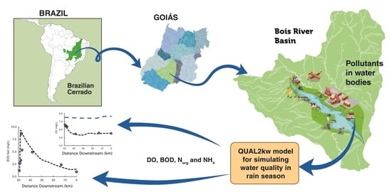
Water Quality Simulation in the Bois River, Goiás, Central Brazil

Abstract

The Cerrado is a hotspot for biodiversity conservation and holds the headwater springs that are major Brazilian river basins. The development of industry, agriculture, and mining causes water quality deterioration. Mathematical models appear as a management tool to simulate water quality parameters and the dispersion of pollutants in water bodies. Thus, this study aimed to evaluate the behavior of dissolved oxygen (DO) and other parameters through the QUAL2Kw (Stream Water Quality Model) model in a river in the Brazilian Cerrado. Complementary data were obtained in four experimental measurement campaigns. The calibration results showed a good fit, especially for the DO. The most critical situation occurred in October, where DO remained below 5 mg/L for a long stretch, and the ammoniacal nitrogen (NH₄) and biochemical oxygen demand (BOD) presented non-compliance concerning the legal Brazilian requirements. In all campaigns, BOD remained above 5 mg/L for at least 5 km in length, disagreeing with the legislation for exceeding the distance from the mixing zone. The uncertainty analysis for the DO confirmed the critical scenario of October, and the sensitivity analysis by the Monte Carlo Simulation showed the significance of the reaeration coefficient for DO. Thus, it is concluded that the QUAL2Kw model proved dependable for the simulation of point launches in the Bois River, supplying a good fit in the calibration act. Because BOD does not meet the legal requirements in all samplings, the water use of the downstream population may be impaired by the activities found in the basin. Activities such as sand extraction, tanneries, and other food industries increase the organic burden of waterbodies and, therefore, require greater environmental inspections.

1. Introduction

The Cerrado biome is a hotspot for the conservation of fauna and flora biodiversity, considered the watershed cradle, as it hosts headwaters that supply a good part of the Brazilian watersheds [1]. Population growth promotes an increase in the use of natural resources to supply the development of economic activities, be it in the industry, farming, and even our domestic use, causing an increase in effluent generation [2]. This scenario might lead to the decrease in hydric bodies’ water quality, as the effluents are sent untreated or, most of the time, treated with low efficiency, increasing the organic load in the source [3,4].

The stabilization of such an organic load sent into hydric bodies consumes dissolved oxygen, altering the aquatic ecosystem’s balance. The sources’ excellent quality of water may be reached through a management strategy which involves the impact evaluation of the pollutants in dissolved oxygen concentration along the river systems [5].

In this context, the assessment of water quality, whether through the Water Quality Index (WQI) in groundwater [6,7,8] or surface water [9,10], using neural networks and machine learning [11,12], or through mathematic models employing computer software are widely used to simulate hydrodynamics, dispersion, and kinetics of pollutants in the natural environment [13]. They allow for the simulation of water usage situations, defining the ability of assimilation through the limits of disposal of finding sources or for the extractions of certain outflows, in a manner that implies calculated risk about the deterioration of water quality according to legal standards [14]. There also exist methods to help choose a more proper model for a determined situation, such as ScoRE (Scope, Record and Experience), which also gives orientation for excluding models [15]. One of the requisites for modeling water quality is to find its adequation for the intended use. Many countries are working to develop guidelines about the investigation and management of water quality and the environment, offering regulated models for the preview of water quality [16].

Therefore, mathematic modeling is an indispensable tool in the search for the preservation of aquatic ecosystems, aiding in maintaining water quality. It helps managers, regulatory bodies, and policymakers direct water bodies’ sustainable planning and management [16].

Several wide models are used to simulate water quality in rivers and creeks, highlighting SIMCAT (SIMulation CATchment), TOMCAT (Temporal Overall Model for CATchments), QUAL2EU (Enhanced Stream Water Quality Model), WASP (Water Quality Analysis Simulation Program), QUASAR (QUAlity Simulation Along Rivers), QUAL2Kw (Stream Water Quality Model), AQUATOX (AQUAtic TOXicology), CE-QUAL-W2 (Hydrodynamic and Water Quality Model), EFDC (Environmental Fluid Dynamics Code), SWAT (Soil and Water Assessment Tool), and SPARROW (SPAtially Referenced Regression On Watershed attributes), among others [5,15,16,17].

The QUAL2Kw (Stream Water Quality Model) includes an automated calibration system and presents the interaction between the constituent parts [1]. It is a modernized version of the QUAL2E model and is a unidimensional model of steady flow, based on solving differential advection–dispersion equations, in all its terms, through an implicit scheme of finite differences, applicable for dendritic rivers [18]. It allows multiple entries, water abstraction in each segment, and the simulation of several parameters [18]. It is (the United States Environmental Protection Agency) US EPA’s official model and is used in several research works to verify the self-depuration of rivers, such as in Brazil [19,20] and other countries, such as the United States of America (USA) [21], Iran [22], and Ethiopia [23]. In addition, it has been shown to be advantageous over other models for a complex river system [24].

The Bois River watershed is of utmost importance for the state of Goiás, as it concentrates on several economic activities. The city of Palmeiras de Goiás, with a population of approximately thirty thousand inhabitants, is supplied with treated water after being sourced from the Bois River. However, upstream it receives untreated domestic sewage and effluents from frigorific warehouses, beverage companies, and tanneries, among others [25]. Besides that, there are several sand extraction points, which cause deforestation in riparian woods and floodplain areas, causing erosion processes, with the increase in water turbidity levels, and chemical pollution caused by oils, greases, and detergents [26]. In 2013, a local television station reported the death of hundreds of fish in the Bois River near the town of Nazário in Goiás, and the probable cause was the discharge from two enterprises, one due to treatment failure and the other due to an overflow [27]. In a study conducted on the Bois River without the use of mathematical models, toxicological tests allowed for the conclusion that its waters seem to be non-toxic to the early life stage of the zebra fish, pointing out that other trophic levels should be studied as they may be suffering from the release of probable pollutants [25].

The pointed contamination causes demand for a sustainable solution for better socioeconomic development [16]. In that way, and considering the need to conduct demands about sending effluents into water bodies, the companies which generate such waste must implement treatment systems to minimize the impacts on the water body and attend to its self-depuration capacity. In addition to using the WQI as a predictor for improving water quality in water to be treated in water treatment plants [28], the application of the QUAL2Kw model on the Bois River might help both private companies and public power in planning and rationalizing the use of such hydric resources, which has already been used in similar scenarios to reduce pollution [23].

Facing what has been exposed, this study has as its goal to evaluate the representability of the model QUAL2Kw to simulate the dissolved oxygen (DO) parameters, biochemical oxygen demand (BOD), organic nitrogen (N_org), and ammoniacal nitrogen (NH₄) in the rainy season of a Bois river’s stretch, in the Brazilian Cerrado.

2. Materials and Methods

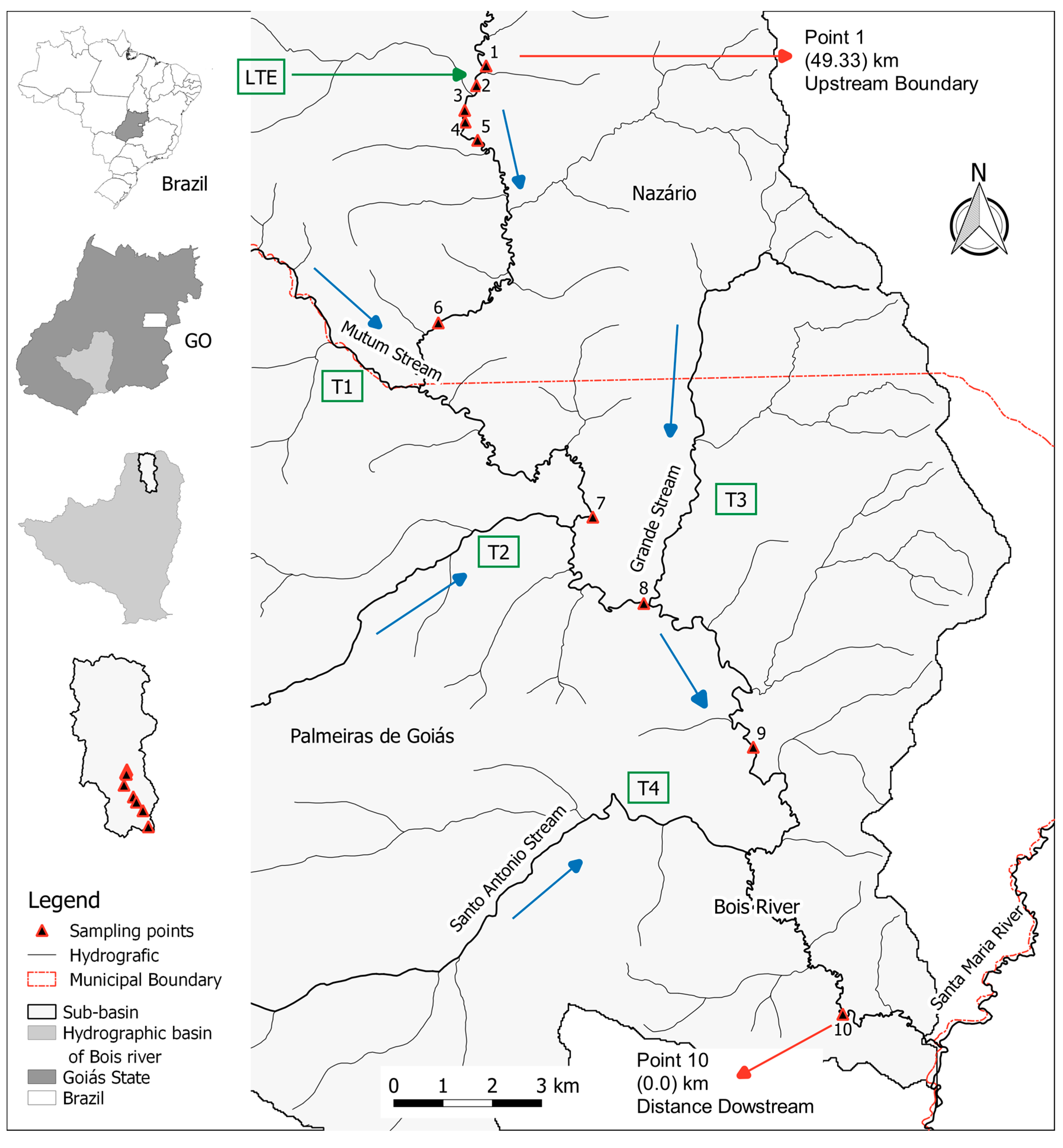
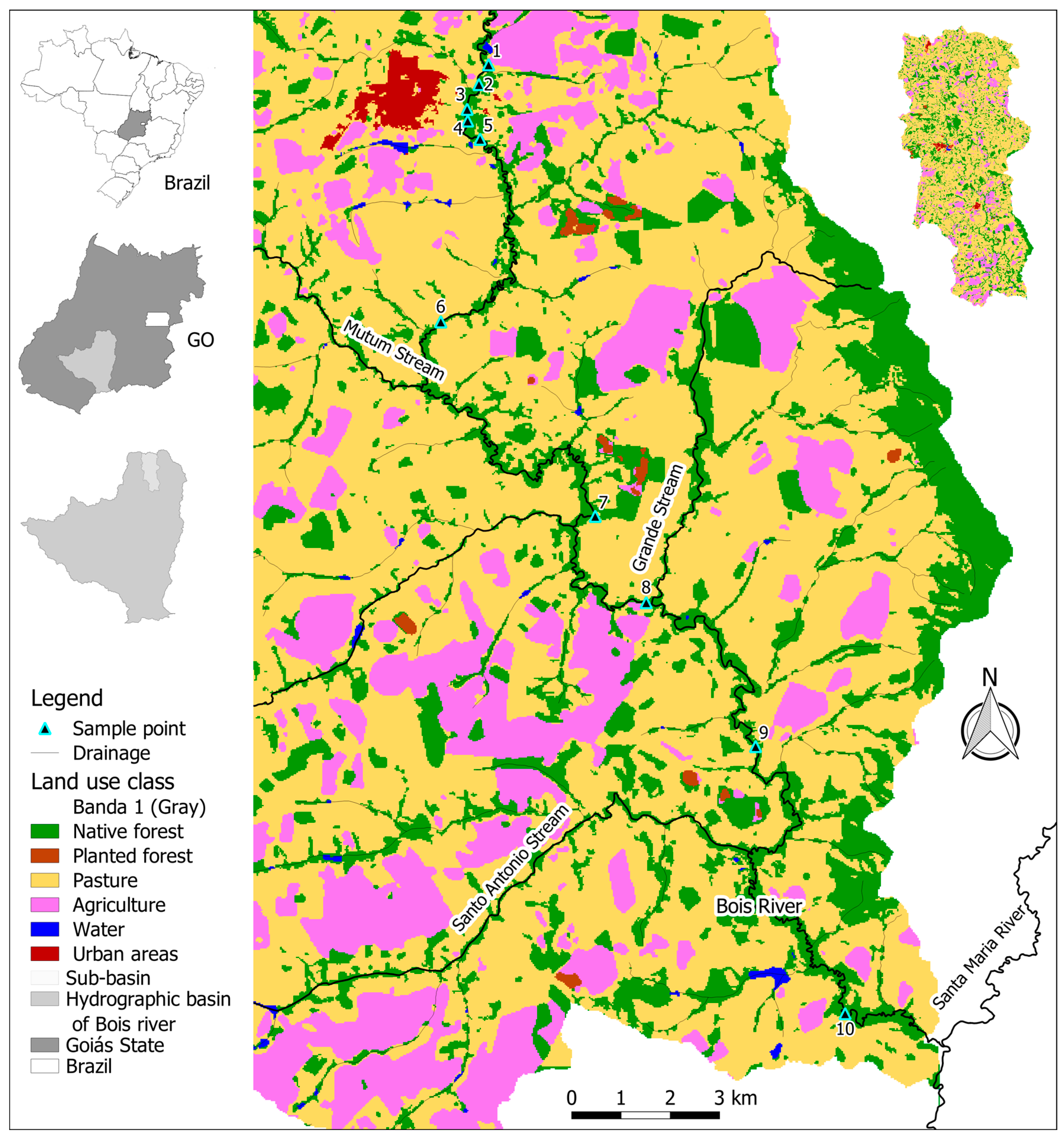
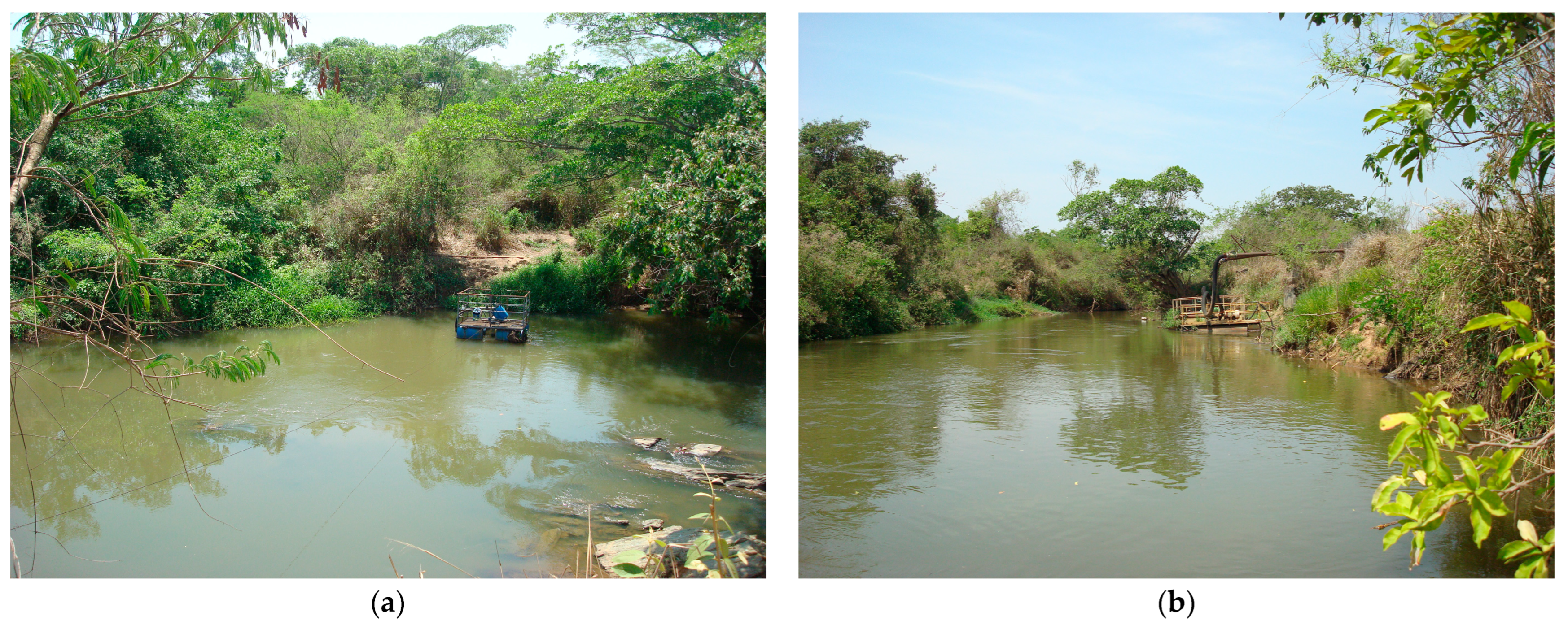
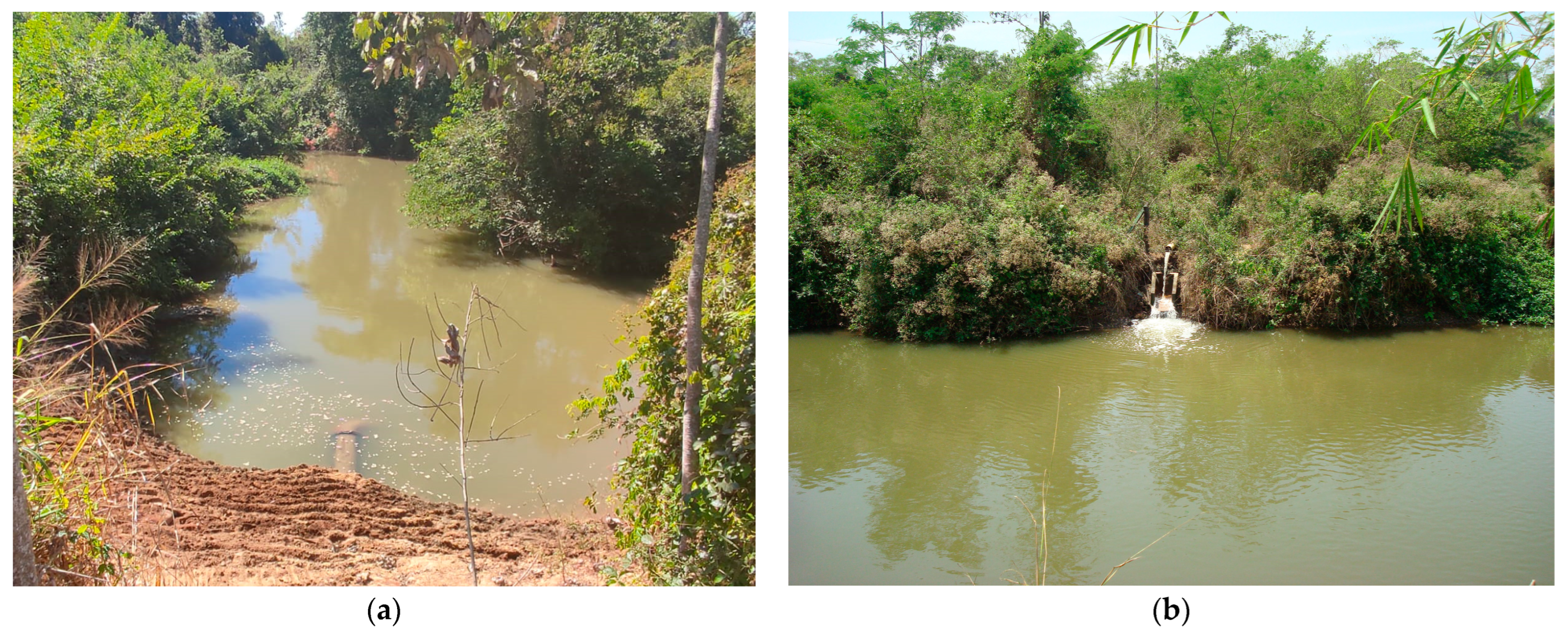
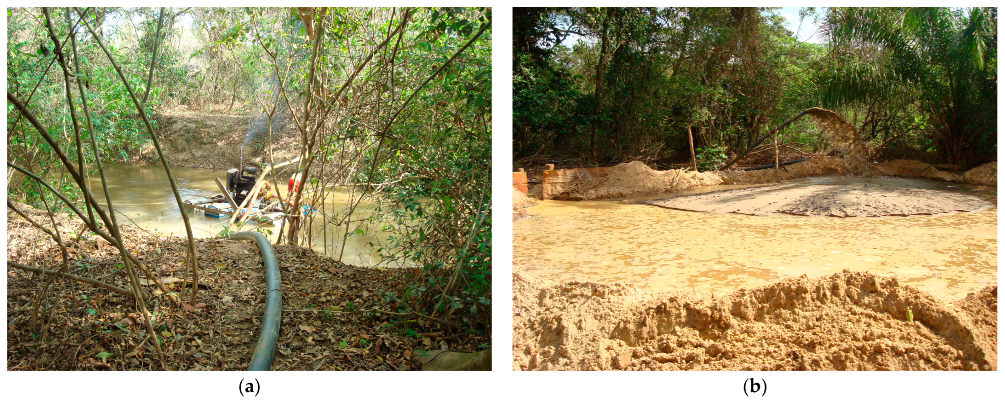
2.1. Study Area

The Bois River watershed reaches 43 municipalities, representing 10% of the population of the state of Goiás, Brazil. This river finds its source in the municipality of Americano do Brasil-GO and runs into the Parnaíba river. Livestock and farming are expressive economic activities, with the use and occupation of the land composing 81% of the watershed’s total area, and one of the main water uses is irrigation [26].

A stretch of 49.3 km (point 1 to point 10) of the Bois River has been analyzed, starting at a point 86 km away from its source (near Nazário-GO) and ending at 4 km of the Santa Maria river’s mouth upstream (near Palmeiras de Goiás-GO) (Figure 1). This stretch is inserted in a sub-basin of 1264.3 km² of the Bois River watershed, which has a total area of 37,189.7 km². In this sub-basin, land use and land cover (LULC) in the agriculture and pasture class reaches up to 82% of the total area (Figure 2). The other classes of use and land cover make up only 17.5% of the native forest area (Cerrado); 0.5% are urban areas and 0.3% are water (

Table 1. Land use and land cover class of the Bois River sub-basin.

LULC—Land Use and Land Cover	Area (%)
Native forest (Cerrado)	17.5%
Planted forest	0.3%
Pasture	69.5%
Agriculture	11.9%
Water	0.3%
Urban areas	0.5%

).

The annual rain average in this area is 1500 mm and the climate is characterized by the type “Aw” [29], which corresponds to the hot tropical climate throughout all the seasons of the year, with a dry winter. A seasonality characteristic can be seen, in which the dry months (May to September) present a monthly rainfall average inferior to 50 mm, while the humid months (October to April) present a monthly average above 100 mm, surpassing 250 mm in December and January.

Being attentive to the release of domestic and industrial sewage in the studied stretch, the water quality of the Bois River will be evaluated by applying the unidimensional QUAL2Kw model. For that, the calibration of such a model with experimental data in the rainfall season and its confirmation in the same season, to avoid distortion in the calibrated constants, have been conducted. The following steps have been taken to feed the model.

The model calibration was carried out in the rainfall season, considering the high flow variations in this season (the most critical condition). The hypothesis was that if the simulation of the model was applied in the rain, it would also have good representation in the dry conditions, due to the more stable flow variation.

2.2. Data and Monitoring Sites

Four collection campaigns have been conducted in the rainfall periods (October/November 2015 and February/March 2016), obtaining the necessary data for the model’s calibration. The water samples have been collected in 10 spots distributed along a stretch with a 49.3 km extension, starting in point 1 (49.33 km upstream boundary) and finishing on point 10 (0.0 km distance downstream) (Figure 1). The spots have been chosen according to the ease of access and from the location of release and abstraction sources found, and all are situated upstream of the water collection area for public supply of the municipality of Palmeiras de Goiás, between the municipalities of Nazário and Palmeiras de Goiás, in the state of Goiás, Brazil.

Among the 10 collection spots, flow measurements have been conducted in 5 spots (2, 4, 6, 9, and 10) (Figure 1). In the first sampling campaign, in October 2015, at the beginning of the rains, it was possible to carry out the flow measurements at points 7 and 8, according to the planning. In the 3 subsequent sampling campaigns, points 7 and 8 were inaccessible, due to excessive rain that prevented the passage on the roads. These spots have been chosen for presenting a flow that is similarly uniform for the conduction of the flow measurement and because of the possibility of access to the river margin. Four of the have been conducted in each spot with the round-trip movement from one margin to the other of the river, using as a result the measurements’ average. The outflows and average speeds have been obtained using the equipment Acoustic Doppler Current Profiler (ADCP) SONTEK brand, model RiverSurveyor M9 [30], which includes a sort of sonar to measure the local depth, GPS for positioning measurement, and a speed sensor.

This equipment is composed of a floating vessel with bathymetric sensors being moved along the transversal section of the watercourse with the aid of ropes, controlled by the research team, which was placed on both riversides (Figure 3). This dynamic measurement allows the visualization of the profile of water speed and depth bathymetry.

The analysis of the water quality parameters was dissolved oxygen (DO), organic nitrogen ($N_{org})$, ammoniacal nitrogen (NH₄), and biochemical oxygen demand (BOD₅) (

Table 2. Sampling point data in October, November 2015 and January, March 2016.

October 2015
Point	Downstream Distance	T	pH	DO	BODfast	Norg	NH4	Q	H	U
	(km)	(°C)		(mgO2/L)	(mgO2/L)	(µgN/L)	(µgN/L)	(m³/s)	(m)	(m/s)
1	49.33	26.97	6.80	6.76	1.65	154.00	476.00	-	-	-
2	48.75	27.03	6.90	6.74	1.81	252.00	280.00	3.56	1.03	0.23
3	48.04	27.07	7.00	6.78	1.81	196.00	224.00	-	-	-
4	47.71	27.30	7.10	6.86	1.07	336.00	448.00	4.04	0.80	0.28
5	47.01	27.30	7.20	6.85	2.47	392.00	392.00	-	-	-
6	38.09	28.67	7.30	5.69	7.75	1484.00	308.00	3.91	0.64	0.34
7	25.92	29.13	7.10	5.07	8.66	700.00	252.00	4.44	0.56	0.44
8	20.42	28.70	7.20	4.86	7.17	196.00	364.00	4.89	0.95	0.23
9	13.13	28.50	7.20	4.56	4.53	168.00	448.00	5.00	1.08	0.22
November 2015
Point	Downstream distance	T	pH	OD	BODfast	Norg	NH4	Q	H	U
	(km)	(°C)		(mgO2/L)	(mgO2/L)	(µgN/L)	(µgN/L)	(m³/s)	(m)	(m/s)
1	49.33	25.87	8.56	6.58	1.73	392.00	168.00	-	-	-
2	48.75	25.88	8.47	6.54	2.23	644.00	84.00	9.33	1.35	0.433
3	48.04	25.75	8.30	6.55	3.63	588.00	84.00	-	-	-
4	47.71	26.73	8.39	6.41	3.22	700.00	196.00	9.95	0.75	0.524
5	47.01	26.17	8.42	6.43	4.20	336.00	224.00	-	-	-
6	38.09	27.47	8.41	5.86	6.51	924.00	196.00	9.86	0.92	0.506
9	13.13	25.98	8.25	5.40	3.63	448.00	112.00	13.27	1.37	0.451
10	0.00	26.09	8.06	4.88	4.45	644.00	84.00	17.99	1.93	0.504
January 2016
Point	Downstream distance	T	pH	OD	BODfast	Norg	NH4	Q	H	U
	(km)	(°C)		(mgO2/L)	(mgO2/L)	(µgN/L)	(µgN/L)	(m³/s)	(m)	(m/s)
1	49.33	26.73	7.10	6.74	3.30	28.00	224.00	-	-	-
2	48.75	26.27	7.48	6.80	2.97	168.00	112.00	12.84	1.36	0.471
3	48.04	26.00	7.68	6.79	4.37	196.00	168.00	-	-	-
4	47.71	26.03	7.81	6.79	5.19	252.00	196.00	13.60	0.95	0.595
5	47.01	26.33	7.03	6.72	6.27	168.00	252.00	-	-	-
6	38.09	26.37	7.98	6.01	11.21	84.00	252.00	-	-	-
7	25.92	26.30	7.95	5.41	5.36	196.00	252.00	-	-	-
9	13.13	26.07	8.15	5.52	4.20	112.00	224.00	15.31	1.38	0.524
10	0.00	26.47	7.25	5.40	2.97	168.00	252.00	15.63	1.70	0.459
March 2016
Point	Downstream distance	T	pH	OD	BODfast	Norg	NH4	Q	H	U
	(km)	(°C)		(mgO2/L)	(mgO2/L)	(µgN/L)	(µgN/L)	(m³/s)	(m)	(m/s)
1	49.33	26.23	7.48	6.61	1.24	112.00	0.00	-	-	-
2	48.75	26.50	7.56	6.45	2.72	280.00	0.00	7.23	0.98	0.325
3	48.04	26.63	7.58	6.42	3.30	70.00	98.00	-	-	-
4	47.71	26.63	7.70	6.47	8.57	280.00	56.00	8.30	0.92	0.489
5	47.01	27.57	7.69	6.36	5.36	420.00	84.00	-	-	-
6	38.09	27.07	7.58	5.47	4.95	224.00	168.00	8.34	0.72	0.446
9	13.13	27.40	7.67	5.59	2.39	336.00	0.00	11.97	1.24	0.436
10	0.00	27.17	7.57	5.54	0.99	406.00	98.00	14.25	1.69	0.459

). These parameters were chosen due to the ease of obtaining research institutions in Brazil, an emerging country still with few investment resources in research. The analyses have been conducted in the laboratory according to standard methods [31], except for temperature (°C), dissolved oxygen (mg/L), and saturation (%), which have been measured in situ through a previously calibrated HQ30d Hach portable oximeter.

2.3. Modeling Tool

The model QUAL2Kw has a general mass balance described by Equation (1), which considers the entrances and exits, longitudinal diffusion, constituent mass generation, and consumption “c_i” in the element “i”, except for the variables related to algae [28].

$$\frac{d{c}_i}{dt}=\frac{Q_{i-1}}{V_i}{c}_{i-1}-\frac{Q_i}{V_i}{c}_i-\frac{Q_{ab,i}}{V_i}{c}_i+\frac{E_{i-1}^{\prime }}{V_i}\left(c_{i-1}-c_i\right)+\frac{E_i^{\prime }}{V_i}\left(c_{i+1}-c_i\right)+\frac{W_i}{V_i}+S_i+\frac{E_{hyp,i}^{\prime }}{V_i}\left(c_{2,i}-c_i\right)$$

(1)

where Wi = external load of the part in the element i (g/d or mg/d), Si = sources and abstractions of the part due to reactions and mass transference mechanisms (g/m³/d or mg/m³/d). The mass exchange between the water surface and sediment zone is given by the exchange of outflows in the element I, being $E_{hyp,i}^{\prime }$ = flow (m³/d) and the difference of concentration on the water surface (c_i) and the sediment zone (c_2,i).

For automatic calibration, the model uses the Genetic Algorithm (GA) to maximize the quality of result adjustments for the model in comparison to the measured data, adjusting all the model state variables [32]. The optimization of the best fit between the simulation and the observed data is performed through the Root Mean Square Error (RMSE) index, that is, by the smallest difference between the model predictions and the observed data for the different parameters analyzed [33]. The program requires an adjustment formula in which, as its result increases, the adjustment value also increases. As the RMSE decreases as the adjustment improves, the use of the inverse of RMSE is suggested [34]. Thus, the GA maximizes the f(x) adequation function, as presented in Equation (2).

$$f\left(x\right)=\left[\sum _{i=1}^q{w}_i\right]\left[\sum _{i=1}^q\frac{1}{w_i}\left[\frac{\frac{{\sum }_{j=1}^m{O}_{i,j}}{m}}{{\left[\frac{\sum _{j=1}^m{\left(P_{i,j}-O_{i,j}\right)}^2}{m}\right]}^{\raisebox{1ex}{$1$}\!\left/ \!\raisebox{-1ex}{$2$}\right.}}\right]\right]$$

(2)

where $O_{i,j}$= observed value, $P_{i,j}$ = predicted value, $m$ = number of pairs of predicted and sampled values, $w_i$ = weighting factor, and $q$ = number of different state variables included in the reciprocal of the weighted normalized RMSE.

2.4. Model Calibration

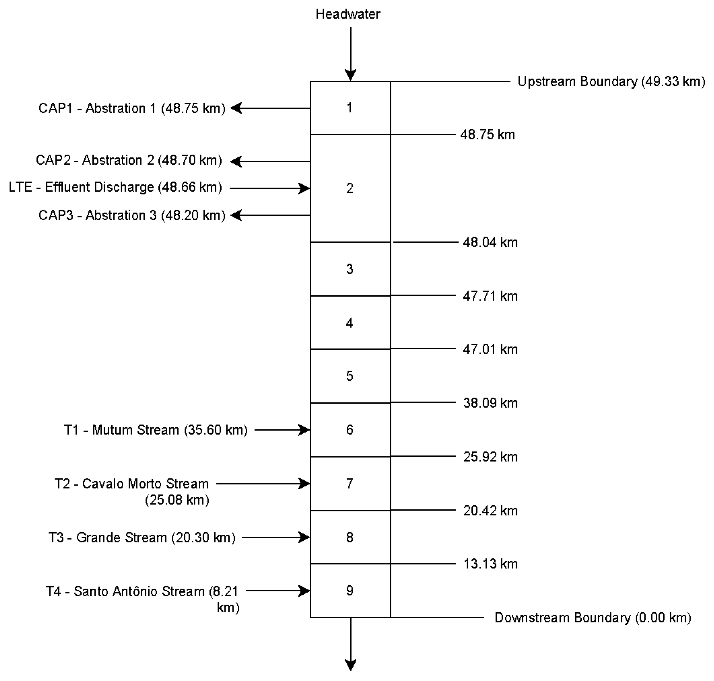
2.4.1. River Discretization

Four relevant tributaries have been considered as punctual releases, respectively titled Mutum Stream, Cavalo Morto Stream, Grande Stream, and Santo Antônio Stream (Figure 1 and Figure 4). The upstream in point 2 has an abstraction point which is the collection from an industry. Between spots 3 and 4, there are two tannery factory collection areas and the respective effluent disposals. Between 4 and 5 are found the waste disposal of a WTS (Water Treatment Station) and the treated effluent of an industry. No other collection spots have been found throughout the studied stretch, such as irrigation pumping, according to the bestowal processes for the use of the Bois River watershed in the state of Goiás for the state’s environmental regulatory body [35].

Since the effluent disposal spots are close to each other, situated in kilometers 48 and 47, for model calibration purposes, a single disposal spot at km 48.66 has been considered, summing up all the effluents disposal loads.

The studied Bois River stretch has been segmented into 9 stretches with distinct distances, for a total of 49.3 km in extension (Figure 4), which presents the unifilar diagram of the main river and the extensions of each stretch, respectively. It is observed that the source of the river coincides with monitoring point 1 and all the point sources are represented, ranging from water abstractions to waste disposals with their respective locations along the main river’s course.

2.4.2. Input Data

The hydraulic characteristics of the studied stretch have been found through classification curves that correlated average speed (U) and depth (H) with the river’s flow (Q) (Equations (3) and (4)):

$$\mathrm{U}=a{\mathrm{Q}}^b$$

(3)

$$\mathrm{H}=\alpha {\mathrm{Q}}^{\beta }$$

(4)

in which, U = average speed (m/s), H = depth (m), a, b, α, and β are empirical coefficients.

The exponents “b” and “β” and coefficients “a” and “α” were calculated for the same sampling spots of the flow measuring (2, 4, 6, 9 e 10) and considered for the stretches defined in the QUAL2Kw (Figure 5). The determination coefficient of Equations (3) and (4) was interpreted using the Pearson Scale, in which 0.00–0.19 is very weak, 0.20–0.39 is weak, 0.40–0.69 is moderate, 0.70–0.89 is strong, and 0.90–1.00 is extraordinarily strong.

The literature reports several conceptual and empirical formulas relating K₂ to the depth and velocity of the watercourse because they are an easily obtainable input data. The QUAL2E model manual [11] records 17 equations and comments that no universal equation is better than the others for all applications. Thus, among the three main equations based on the velocity and depth of the watercourse [36,37,38] and that have ranges of action that complement each other, the formula of O’Connor and Dobbins [36] is the one that fits the conditions of the studied river stretch.

The reaeration coefficients K₂ (

Table 4. K₂ values in function of speed and depth, distributed in 5 collection points in the months of October 2015, November 2015, January 2016, and March 2016.

Sample Point	Month/Year
	October 2015			November 2015
	U	H	K2	U		H	K2
	(m.s−1)	(m)	(d−1)	(m.s−1)		(m)	(d−1)
2	0.23 ± 0.01	1.15 ± 0.02	1.53 ± 0.01	0.43 ± 0.03		1.58 ± 0.17	1.31 ± 0.15
4	0.28 ± 0.01	1.00 ± 0.04	2.08 ± 0.03	0.52 ± 0.02		1.21 ± 0.04	2.14 ± 0.03
6	0.34 ± 0.01	0.83 ± 0.05	3.05 ± 0.02	0.51 ± 0.02		1.220.12	2.06 ± 0.06
9	0.22 ± 0.01	1.20 ± 0.01	1.40 ± 0.01	0.45 ± 0.01		1.50 ± 0.01	1.44 ± 0.01
10	-	-	-	0.50 ± 0.07		2.26 ± 0.08	0.82 ± 0.13
Sample Point	Month/Year
	January 2016				March 2016
	U	H	K2	U		H	K2
	(m.s−1)	(m)	(d−1)	(m.s−1)		(m)	(d−1)
2	0.47 ± 0.01	1.64 ± 0.03	1.29 ± 0.02	0.33 ± 0.01		1.38 ± 0.02	1.39 ± 0.02
4	0.60 ± 0.02	1.37 ± 0.02	1.89 ± 0.01	0.49 ± 0.05		1.20 ± 0.12	2.09 ± 0.10
6	-	-	-	0.45 ± 0.00		1.27 ± 0.00	1.84 ± 0.00
9	0.52 ± 0.00	1.49 ± 0.01	1.56 ± 0.01	0.44 ± 0.01		1.40 ± 0.01	1.57 ± 0.01
10	0.46 ± 0.03	2.19 ± 0.09	0.82 ± 0.05	0.46 ± 0.05		2.04 ± 0.07	0.91 ± 0.07

) to find the O₂ concentrations have been calculated for each river stretch according to the values of depth and speed measured in the watercourse. That way, the O’Connor and Dobbins empirical model [36] presented in Equation (3) has been applied, and it has an approximated application band for speed varying between 0.05 m/s and 0.8 m/s, and depth between 0.6 m and 4.0 m.

$$K_2=3.93{\mathrm{U}}^{0.5}{\mathrm{H}}^{-1.5}$$

(5)

The coefficients which integrate the nitrification phenomenon were calibrated in a chart, using Microsoft Excel’s Solver tool, then inserted in the QUAL2Kw model in the “Reach Rates” chart.

For such, Equations (4) and (5) have been used to simulate the concentration of organic nitrogen and ammoniacal nitrogen with random constant values along with the group of data of each sampling campaign. For the coefficients $R_{{\mathrm{O}}_{2}amon}$, the admitted value was of 4.3 mg O₂/mg N_amon and for K_nitrOD the value of 0.6 L/mg [32].

$$N_{org}=N_{org0} e^{-K_{oa} t}$$

(6)

$$N_{amon}=N_{amon0} e^{-K_{an }t}+\frac{K_{oa} N_{org0}}{K_{an}-K_{oa}}(e^{-K_{oa} t}-e^{-K_{an} t})$$

(7)

Next, the optimization of the constant’s ballots through the minimization of error between the observed and simulated values. The error was calculated from the square of the difference between the observed values with the estimated values by the simulation.

2.4.3. Model Implementation

The calculation time assumed was of 5.625 min using the Runge–Kutta integration method. Fifteen days were adopted for the repetition of simulations and the solution method adopted for the pH was the Newton–Raphson one. The sediment diagenesis and hyporheic zone simulation were disregarded because their contribution to the dissolved oxygen consumption was too small [32].

In the hydraulic model QUAL2Kw (“REACH” tab), discharge coefficients α, β, a, and b of each studied section were released. In the “REACH RATES” tab, the average of K₂ values obtained in the sampling campaigns of October/November 2015 and February/March 2016 was inserted, to be calibrated by the model. In the same tab, the values for K₁ = 0.1 were inserted for every segment of the stretch, where we have the usual values of this constant for watercourses with clean waters varying from 0.08 to 0.20 [39]. The constants of conversion of organic nitrogen to ammoniacal (K_oa) and ammoniacal nitrogen to nitrate (K_an) were also inserted and calibrated for the sampling campaign.

The entry data for the punctual loads found in the studied stretch were inserted in the “Point Sources” tab, where the location of the disposal into the stretch must be mentioned, as well as the flow and the respective quality data for each source (

Table 3. Values applied in the Point Sources tab to perform model calibration in October, November 2015, and January, March 2016.

October 2015
Point		Location	Q	T	DO	BOD	Norg		NH4		pH
Source		(km)	(m³/s)	(°C)	(mgO2/L)	(mgO2/L)	(µgN/L)		(µgN/L)
CAP1		48.75	0.056	-	0.00	0.00	0.00		0.00		-
CAP2		48.70	0.042	-	0.00	0.00	0.00		0.00		-
LTE		48.66	0.138	28.00	1.00	300.00	90000.00		50.00		7.00
CAP3		48.20	0.014	--	0.00	0.00	0.00		0.00		--
T 1		35.60	0.530	28.00	6.80	1.00	0.00		0.00		7.00
T 2		25.08	0.450	28.00	6.80	1.00	0.00		0.00		7.00
T 3		20.30	0.110	28.00	6.80	1.00	0.00		0.00		7.00
T 4		8.21	0.802	28.00	6.80	1.00	0.00		0.00		7.00
November 2015
Point	Location		Q	T	DO	BOD		Norg		NH4	pH
Source	(km)		(m³/s)	(°C)	(mgO2/L)	(mgO2/L)		(µgN/L)		(µgN/L)
CAP1	48.75		0.056	--	0.00	0.00		0.00		0.00	-
CAP2	48.70		0.042	-	0.00	0.00		0.00		0.00	--
LTE	48.66		0.138	26.00	2.00	600.00		80000.00		300.00	8.00
CAP3	48.20		0.014	--	0.00	0.00		0.00		0.00	-
T 1	35.60		1.337	27.00	6.80	2.00		0.00		0.00	8.50
T 2	25.08		1.135	27.00	6.80	2.00		0.00		0.00	8.50
T 3	20.30		0.939	27.00	6.80	2.00		0.00		0.00	8.50
T 4	8.21		4.720	27.00	6.80	2.00		0.00		0.00	8.50
January 2016
Point	Location		Q	T	DO	BOD		Norg		NH4	pH
Source	(km)		(m³/s)	(°C)	(mgO2/L)	(mgO2/L)		(µgN/L)		(µgN/L)
CAP1	48.75		0.056	--	0.00	0.00		0.00		0.00	--
CAP2	48.70		0.042	--	0.00	0.00		0.00		0.00	--
LTE	48.66		0.138	26.00	2.00	900.00		50000.00		3000.00	8.50
CAP3	48.20		0.014	-	0.00	0.00		0.00		0.00	-
T 1	35.60		0.284	27.00	6.80	2.00		0.00		0.00	8.00
T 2	25.08		0.290	27.00	6.80	2.00		0.00		0.00	8.00
T 3	20.30		1.132	27.00	6.80	2.00		0.00		0.00	8.00
T 4	8.21		0.320	27.00	6.80	2.00		0.00		0.00	8.00
March 2016
Point		Location	Q	T	DO	BOD	Norg		NH4		pH
Source		(km)	(m³/s)	(°C)	(mgO2/L)	(mgO2/L)	(µgN/L)		(µgN/L)
CAP1		48.75	0.056	-	0.00	0.00	0.00		0.00		-
CAP2		48.70	0.042	-	0.00	0.00	0.00		0.00		-
LTE		48.66	0.138	26.00	2.00	700.00	30000.00		100.00		7.00
CAP3		48.20	0.014	-	0.00	0.00	0.00		0.00		-
T 1		35.60	1.589	27.00	6.80	2.00	0.00		0.00		7.50
T 2		25.08	1.891	27.00	6.80	2.00	0.00		0.00		7.50
T 3		20.30	0.150	27.00	6.80	2.00	0.00		0.00		7.50
T 4		8.21	2.280	27.00	6.80	2.00	0.00		0.00		7.50

).

The tributaries outflows were estimated through the balance of entrances and releases through the outflows measured in collection points. The collection outflows were obtained through available bestowals in the environmental regulatory body of the state of Goiás, Brazil [35]. The LTE flow was estimated and fixed for every month and the load concentrations were estimated for each sampling campaign in a way to obtain the best adjustment, as well as the DO, BOD, and pH values, as well as the temperature of the tributaries.

The measured BOD in the analyses was the 5-days BOD, which has been transformed into the BOD last (BODu) and inserted in the model for the calculation of BOD_fast (Equation (6)). The BOD_slow was considered null.

$$\mathrm{BOD}\mathrm{u}=\frac{{\mathit{BOD}}_5}{1-e^{-K_{1}5}}$$

(8)

in which, BOD₅ = Biochemical Oxygen Demand in the 5th day, at 20 °C, K₁ = deoxygenation coefficient (day⁻¹).

2.5. Uncertainty and Sensitivity Analysis

To evaluate the DO result in sampling campaigns, a Monte Carlo Simulation has been conducted in distinct distances for the outreach of the 4 calibrated models, with 1000 rounds each, using the normal distribution. Among the evaluated parameters we have LTE flow (QLTE), the DO, and saturation concentration (Cs) in the river, K₁, and K₂. These parameters had certain percentage variations around the fixed value, reflecting the greater or smaller uncertainty level, thus granting a vast range of values.

For such, Q_LTE and K₁ have been varied in 30%, DO in the river in 10%, Cs in 5%, and K₂ in 50%. There is no uncertainty about river course distance, and in this case, the null percentage variation was adopted. On the other hand, the uncertainty in the coefficient K₂ is high, for being empirically found.

In this study, the uncertainty analysis through Monte Carlo Simulation with normal distribution has also been conducted and conducted in the DO model for the coefficients K₁ and K₂ in each sampling campaign using the same parameters and varying percentages of the uncertainty analysis conducted in the earlier item. The data were separated into two groups of samples for 1000 simulations, in which the first 500 values of all data are associated with DO_mín to below the median (Group 1) and the last 5000 values are associated with DO_mín above the median (Group 2).

The uncertainty and sensitivity analysis using Monte Carlo simulation was also applied in Osan Creek, South Korea, together with the QUAL2Kw model, to determine the performance of the model. For each output, the model can produce histograms, frequencies, error bars, and probability density functions [40]

3. Results and Discussion

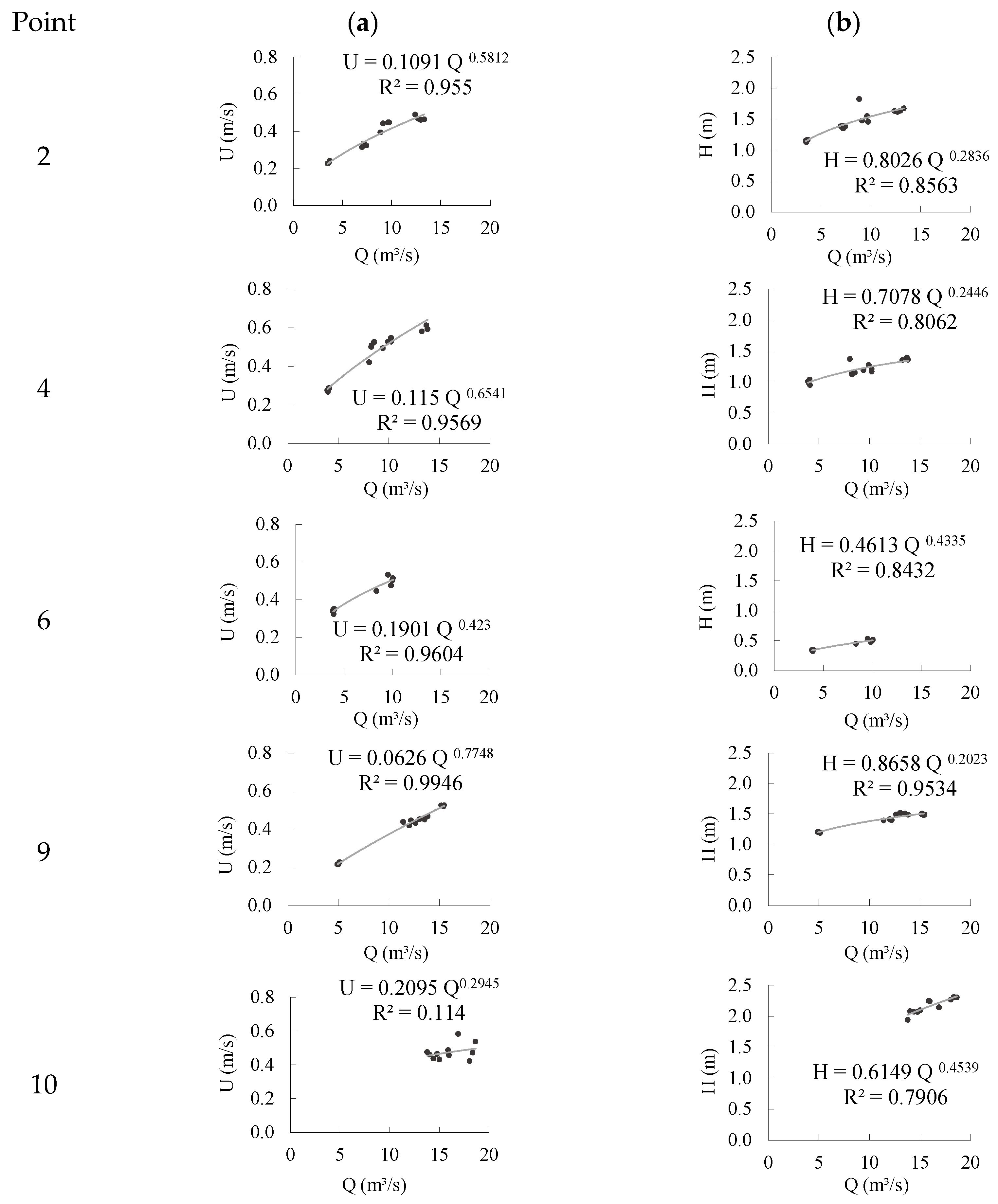
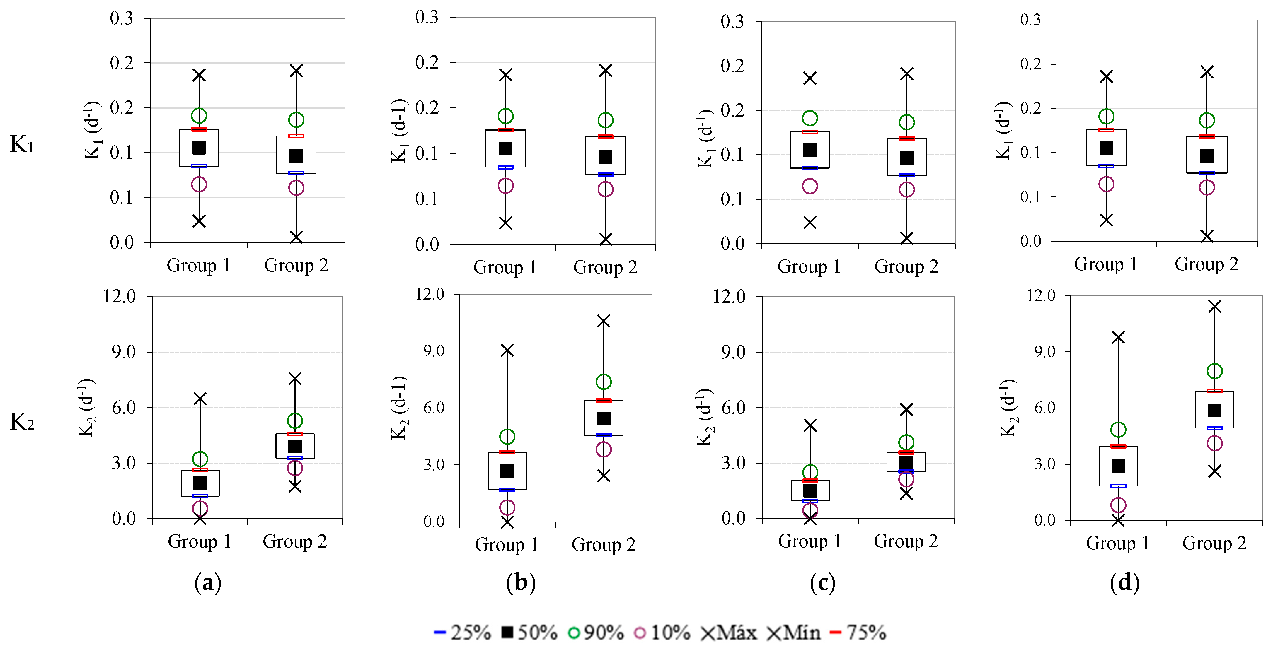
3.1. Reaeration Rate

The unload coefficients result about speed (U) and depth (H), after applying the empirical model of O’Connor and Dobbins [36], are presented in Figure 5. The determination coefficient according to Pearson’s scale of correlation varied from a strong to extraordinarily strong correlation in all points, except for point 10 (correlation very weak between speed and flow (Figure 5a) at point 10).

Despite the weak correlation in finding unloading coefficients at point 10, the O’Connor and Dobbins empirical equation [36] keeps being the most adequate for presenting trustworthy relations for the hydraulic variables of speed and depth, which present more sensitivity and a strong relationship with the reaeration coefficient [41].

However, even the equations of better performance show great preview errors of at least 40–50% and, in a few regions, more than 100% for the reaeration coefficients. This level of preview error in the coefficients of reaeration rate will continue to greatly impact the uncertainty of previews of dissolved oxygen upon applying the water quality models [42].

The reaeration coefficient values obtained have an average of 1.62 d⁻¹, minimum value of 0.82 d⁻¹, and maximum value of 3.05 d⁻¹, with interval of 2.24 d⁻¹ (Table 4). In the southeast of Brazil, the K₂ values varied from 16.94 to 373.79 d⁻¹ [43], values above the ones found in this study, it has been observed that the models developed for temperate aquatic systems may underestimate the K₂ in tropical flows, bringing uncertainty to model metabolic rates, self-depuration capacity, or whatever other processes which depend on reaeration [28].

3.2. Nitrification Rate

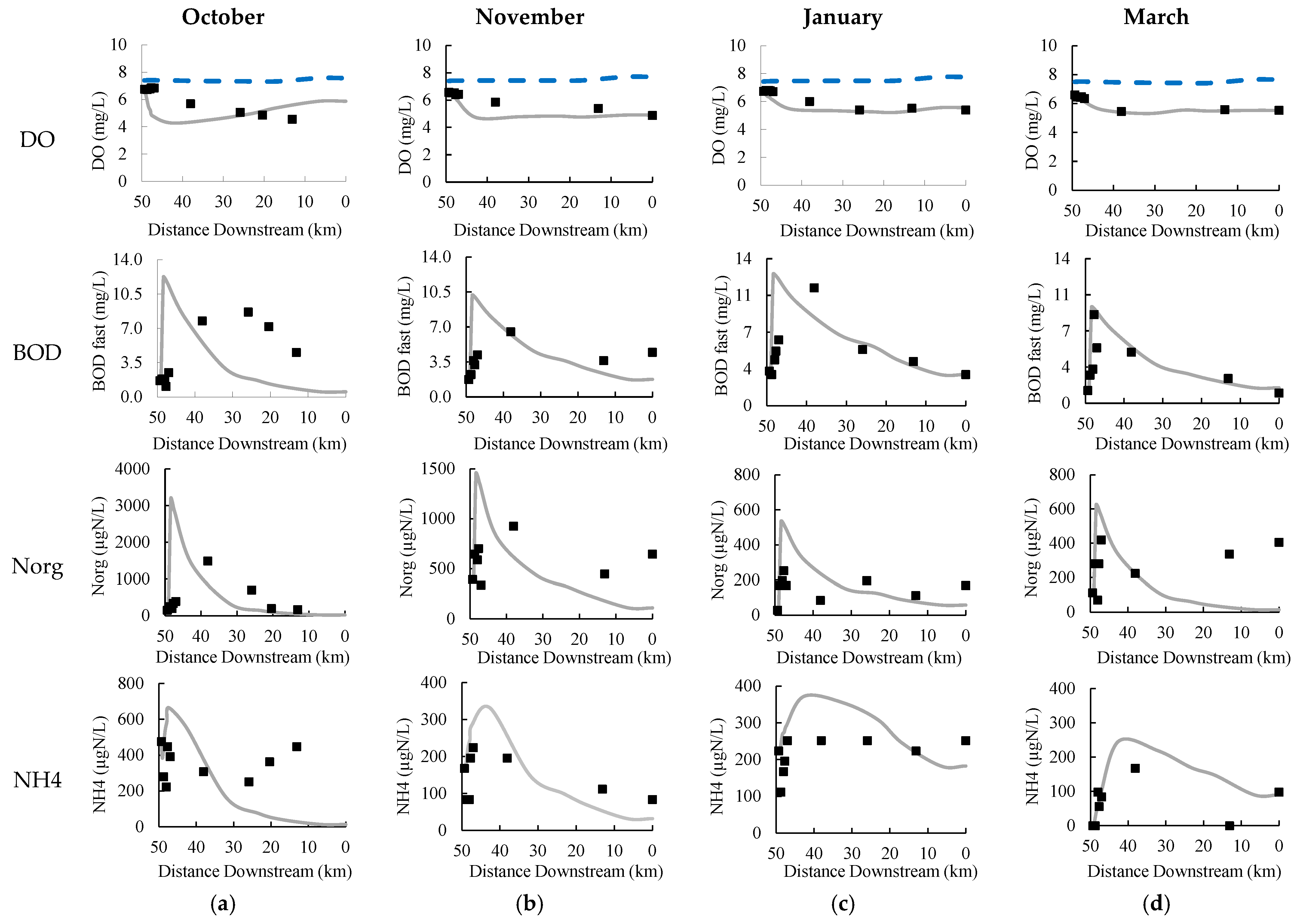
After the calibration of nitrification constants, the obtained result was the values and errors for each sampling campaign (

Table 5. Result of the calibration of the constant of organic nitrogen to ammoniacal (K_oa) and the constant of conversion of ammoniacal nitrogen straight to nitrate (K_an) and their respective errors.

Month/Year	Koa	Error	Kan	Error
October 2015	0.25	2.4743	0.20	0.0702
November 2015	0.20	0.3124	0.77	0.0242
January 2016	0.20	0.0372	1.00	0.0951
March 2016	0.25	0.1490	1.00	0.0309

).

The values obtained in this study (Koa between 0.20 and 0.25; and Kan between 0.20 and 1.00) are in line with the calibrated constants in the application of the QUAL2K model to identify the contribution of ammonia nitrogen pollution from various sources. The authors obtained values between 0.25 and 0.30 for the constant Koa and 0.22 to 0.28 for the constant Kan [44].

3.3. Calibration

The model calibration was conducted by the genetic algorithm, using 100 generations and 100 simulations within the same population once the increase in these parameters does not result in sensible gains in adjustment quality [32]. The other parameters used in the optimization of the PIKAIA genetic algorithm were values defined as standard by the model.

After auto-calibration, the estimation of concentrations of the total nutrient load of the disposal of effluents were estimated, to obtain the best value for the reverse of the average root of errors squared RMSE of each sampling campaign. The reaeration was simulated by the model’s internal form, in which the method was selected according to depth and speed relations.

The inverse RMSE obtained by the auto-calibration was of 0.8055 for October 2015, 0.8153 for November 2015, 0.8026 for January 2016, and 0.8080 for March 2016.

The average of the inverse of the RMSE obtained in the calibration adjustment of the model for the study section and for all the sample campaigns was 0.8154. The higher the adjustment value (closer to 1), the more accurate the model will be. The RMSE obtained by other researchers calculated for the model calibration showed good compatibility (95%) between the observational and predicted data [22,45,46,47]. Therefore, the data were associated with a high level of accuracy. However, another study presented a lower adjustment value, around 0.65 [48].

The calibration results for October 2015 (Figure 6a) had a good adjustment when compared to the observed values, with value of the RMSE inverse of 0.8055. Regarding the DO, the model simulates concentrations which reach a value of 4.40 mg/L and stay below 5 mg/L through around 24 km of the stretch’s extension. The DO concentration has a different behavior in comparison to other months, and about the measured data, as it simulates starting from km 20, the recovery zone of the DO concentrations, while the data still decline.

The simulated BOD reaches a maximum value of 12.25 mg/L right after the LTE disposal point and stays above 5 mg/L for 5 km of longitudinal extension of the river. In the same way as DO, the measured data in the field for BOD have an atypical behavior, where there is no exponential decay of the values. This behavior can be justified by the existence of diffuse contributions, which were not considered in the simulation and can contribute to the decay of DO data and increase in field BOD data [49].

Norg does not have the standard limits recommended by CONAMA 357/2005 [46] and has a good visual fit of field-measured data to simulated data. However, the NH₄ levels remained above 500 µg/L, with a peak of 664.59 µg/L, in the same range as BOD failed to comply with the law [50]. The NH₄ values measured in the field initially showed high concentrations, decreased, and then increased again halfway through the route, which is inconsistent with the behavior of other months, which remain constant or continued to decrease until the end of the stretch. The increase in NH₄ load is related to several pollution sources, mainly livestock confinement, followed by agricultural production, rural families, industry, and soil erosion [44].

In November 2015, the calibrations results (Figure 6b) reached the value of 0.8153 as RMSE inverse to evaluate the model’s adjustment. The DO simulated concentrations present themselves below the recommended standards [50], reaching a minimum value of 4.65 mg/L at km 32. The simulation remained below the concentrations measured on the field. This degradation of quality is attributed to the existence of pollutant loads received from upstream parts of the river that were not identified, as seen in the Gheshlagh River in Iran [51]. This behavior may be justified too by the process of reaeration being higher than the one simulated by the model, once that K₂ is a determinant in the DO concentrations.

The BOD reaches its peak at 10.19 mg/L, after the LTE point, and stays above the recommended standard through 5.84 km of its extension, following the tendency of the observed data on the field. The other parameters are within the recommended values by the current law, but the tendency of the data seen by Norg increased past km 25, while the ones in the model have decayed. Other authors have found that besides the oxidation rate, the nitrification and denitrification rates also have a significant influence on the simulation of water quality [52].

In the month of January 2016, the calibration results (Figure 6c) also obtained a good adjustment with the RMSE inverse value of 0.8026 and followed the tendencies of data seen on the field. Most calibrated parameters kept themselves within the recommended standards [50], except for the BOD, which lasted above 5 mg/L for approximately 25 km of the river’s stretch, with a maximum value of 12.55 mg/L at 48.4 km away from downstream, after the LTE point. Studies indicate that the critical conditions of the BOD parameter originate from sources of agricultural wastewater discharge [44].

In March 2016 (Figure 6d), the calibration generated a value of the RMSE inverse of 0.8080. In the same way, as in January 2016, most calibrated parameters were within the standard conditions [50], except for the BOD, which reached a peak of 9.32 mg/L and remained above 5 mg/L for 5.84 km of extension.

In all sampling campaigns, the BOD remained above 5 mg/L for at least 5 km, being in discrepancy with the legislation, once it allows values above the standard up to the course distance to reach a total mixture (mixture zone). Considering the disposal of sewers in a margin and using the Yotsukura method [53] for the finding of the mix zone for the river section after the disposal of effluents (point 40), there is an average of 1.5 ± 0.5 km until reaching the mixture zone.

The application of the QUAL2Kw model reproduces, in a general manner, the expected behavior for the analyzed parameters (Figure 6), except for a few punctual results. This is due to the complexity of the analyzed problem, taking the uncertainties into consideration associated to the disposal loads, diffuse loads, and flow variations (flow control) [54]. In addition to diffuse loads, other studies attribute these changes to contributions from groundwater, which can be simulated in QUAL2Kw as diffuse loads in the model, which was not carried out in this article [55].

Certain errors were reported for being unavoidable because only one sample is collected per day, so the simultaneous sampling in each point cannot be guaranteed. However, the water quality may vary depending on the sampling time throughout the day [56].

Moreover, the application of the model in the rain made it difficult to calibrate the model, mainly because of the difficulty of estimating the effluent loads, whether from point sources or diffuse ones that were accentuated because of the surface runoff.

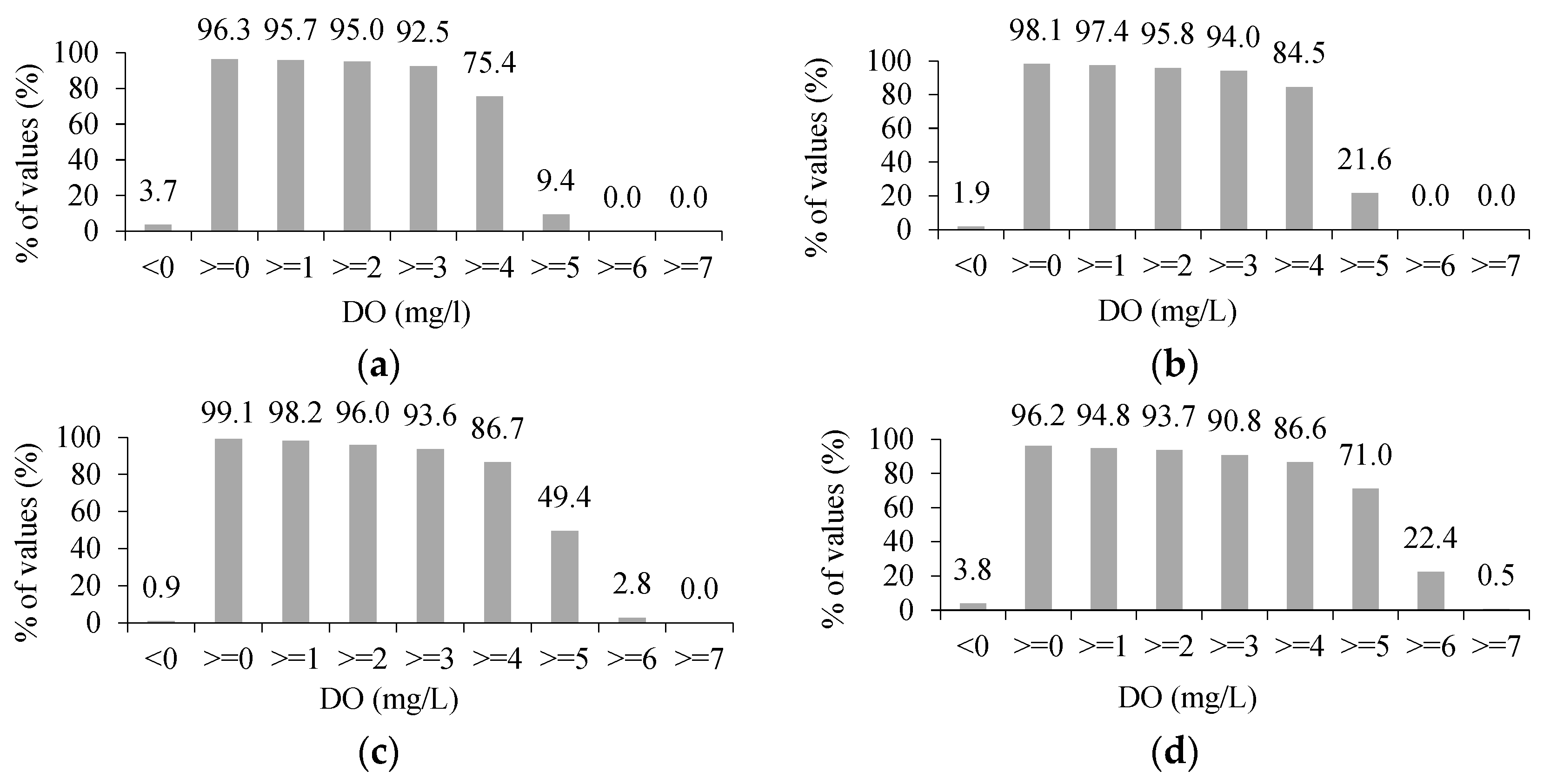
3.4. Uncertainty and Sensitivity Analysis

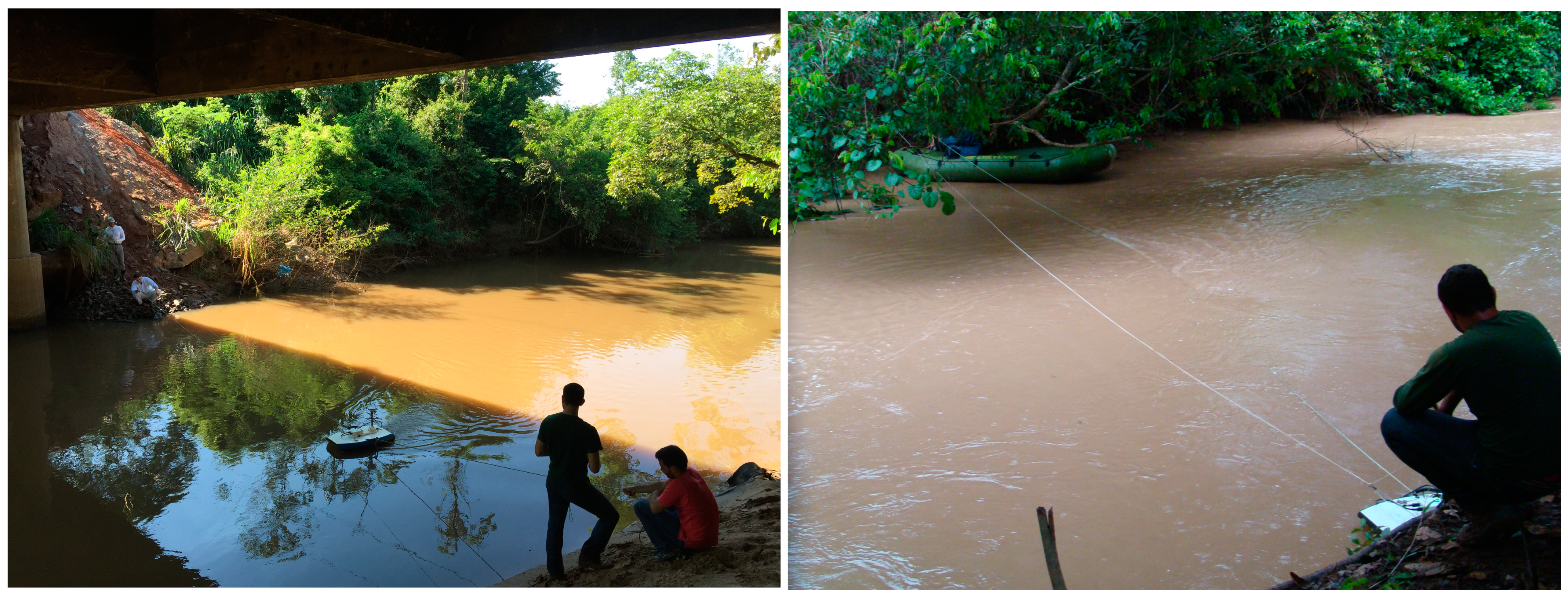
The uncertainty analyses results are represented as accumulated frequency distribution of the DO parameter (Figure 7) for the sampling campaigns of October 2015 at km 32.00, November 2015 at km 42.55, January 2016 at km 16.77, and March 2016 at km 47.36, respectively.

These results show that in the month of October 2015 (Figure 7a), only 9.4% of the simulations led to the regulatory compliance for Class 2 water bodies and that 66% of the simulations led to an OD_mín between 4 and 5 mg/L. In the month of November 2015 (Figure 7b), there is a 21.6% probability that the sewage disposal will lead to compliance, within the assumed conditions, and 62.9% of the simulations led to the OD_mín value between 4 and 5 mg/L. In January/2016 (Figure 7c), the scenario improves with the percentage of regulatory compliance, which raises to 49.4%, and the OD_mín stayed within the values of 5 and 6 mg/L with a 46.6% probability. The best scenario of compliance with the regulation happens in the month of March 2016 (Figure 7d), where 71% of the simulations for the OD_mín are found above 5 mg/L, with a 48.6% probability of staying within the values between 5 and 6 mg/L, and 21.9% of simulations leading to 6 and 7 mg/L.

The sensitivity analysis results (Figure 8) show that for all the sampling campaigns, through visual analysis, the K₁ results in Group 1 and 2 do not have significant differences, where the average of both samples tends to be equal and the K₁ value is not a determinant in the OD_mín values. However, the K₂ values in Group 2 samples of all the sampling campaigns are associated with much higher values than in Group 1 sample, being significantly different. With basis on the non-parametric t-test, it has been confirmed that there are differences between the sampling groups 1 and 2, for the K₂ variable, with a 5% (p ≤ 0.05) significance; that is, the K₂ coefficient is a determinant for the OD_mín results.

3.5. Difficulties

The Bois River receives various discharges and has extractive activities that may complicate the application of a model. After the model was applied, a visit was made to the Bois River in order to comprehend the results. During the visit, it was noted that, in addition to locations with water supply for industrial (Figure 9a,b) and human consumption (Figure 10a), there was also the discharge of effluents (Figure 10b), as well as the removal of sand (Figure 11a) and its processing (Figure 11b) for use in construction. Other withdrawals of water, whether for local agriculture and livestock, can occur in the Bois River and may influence the model, as has already been observed in other studies [45].

4. Conclusions and Recommendations

The goal of this study was to evaluate the representability of the QUAL2Kw model to simulate the DO, BOD, and other quality parameters for water quality in the rainfall season of a stretch of river in the Brazilian Cerrado. This model is used for small rivers with flow conditions of a stationary state.

The DO concentration remained below 5 mg/L for a long stretch, in October, when the flow was the lowest. The BOD and NH₄ presented greater concentration and did not follow the Brazilian legal requirements. BOD remained above 5 mg/L in an extension of at least 5 km in all sampling campaigns.

Regarding the water quality simulation results, which do not follow the legal requirements of a few parameters in all samples, the use of downstream water by the population might be harmed by the activities conducted in the Bois River watershed. The activities increase the spring source’s organic load, thus needing greater environmental inspection.

The model QUAL2Kw, despite showing good adjustment in the calibration act, also showed high dispersion between data collected in the field and simulated data for the Bois River in the rainfall season. The most critical scenario happened in the smallest flow detected at the source, where the greatest concentration of pollutants was seen. Despite that, the model will aid in the management of surface waters in the rivers of the Cerrado in Goiás. The sensitivity analysis exposed and confirmed how significant the reaeration coefficient is in the determination of DO concentrations.

The main difficulties faced from data collection to analysis and understanding of results were limited resources for acquiring samples and laboratory analysis and finding studies in regions with similar characteristics that presented the same conditions for applying the model.

The recommendations for future works are to estimate the downstream diffuse load of the effluent disposal points to reduce the uncertainty about punctual load; and to extend the studied stretch throughout the river to evaluate the behavior of DO in the recovery zone.

References

1. Borma, L.S.; Costa, M.H.; da Rocha, H.R.; Arieira, J.; Nascimento, N.C.C.; Jaramillo-Giraldo, C.; Ambrosio, G.; Carneiro, R.G.; Venzon, M.; Neto, A.F.; et al. Beyond carbon: The contributions of South American tropical humid and subhumid forests to ecosystem services. Rev. Geophys. 2022, 60, e2021RG000766. [Google Scholar] [CrossRef]
2. Gude, V.G.; Gadhamshetty, V.; Ramanitharan, K. Sustainable Water: Resources, Management and Challenges; Nova Science Publishers, Inc.: New York, NY, USA, 2020; 259p. [Google Scholar]
3. Zagklis, D.P.; Bampos, G. Tertiary Wastewater Treatment Technologies: A Review of Technical, Economic, and Life Cycle Aspects. Processes 2022, 10, 2304. [Google Scholar] [CrossRef]
4. Zhang, Z.; Deng, C.; Dong, L.; Zou, T.; Yang, Q.; Wu, J.; Li, H. Evaluating the anthropogenic nitrogen emissions to water using a hybrid approach in a city cluster: Insights into historical evolution, attribution, and mitigation potential. Sci. Total Environ. 2023, 855, 158500. [Google Scholar] [CrossRef]
5. Kannel, P.R.; Kanel, S.R.; Lee, S.; Lee, Y.-S.; Gan, T.Y. A Review of Public Domain Water Quality Models for Simulating Dissolved Oxygen in Rivers and Streams. Environ. Model. Assess. 2011, 16, 183–204. [Google Scholar] [CrossRef]
6. Kouadri, S.; Elbeltagi, A.; Islam, A.R.M.T.; Kateb, S. Performance of machine learning methods in predicting water quality index based on irregular data set: Application on Illizi region (Algerian southeast). Appl. Water Sci. 2021, 11, 190. [Google Scholar] [CrossRef]
7. Li, M.; Li, B.; Chu, J.; Wu, H.; Yang, Z.; Fan, J.; Yang, L.; Liu, P.; Long, J. Groundwater Quality Evaluation and Analysis Technology Based on AHP-EWM-GRA and Its Application. Water Air Soil Pollut. 2023, 234, 1–18. [Google Scholar] [CrossRef]
8. El Yousfi, Y.; Himi, M.; El Ouarghi, H.; Aqnouy, M.; Benyoussef, S.; Gueddari, H.; Ait Hmeid, H.; Alitane, A.; Chaibi, M.; Zahid, M.; et al. Assessment and Prediction of the Water Quality Index for the Groundwater of the Ghiss-Nekkor (Al Hoceima, Northeastern Morocco). Sustainability 2023, 15, 402. [Google Scholar] [CrossRef]
9. Tharmar, E.; Abraham, M.; Prakash, R.; Sundaram, A.; Flores, E.S.; Canales, C.; Alam, M.A. Hydrogeochemistry and Water Quality Assessment in the Thamirabarani River Stretch by Applying GIS and PCA Techniques. Sustainability 2022, 14, 16368. [Google Scholar] [CrossRef]
10. Azhari, H.E.; Cherif, E.K.; Sarti, O.; Azzirgue, E.M.; Dakak, H.; Yachou, H.; Esteves da Silva, J.C.G.; Salmoun, F. Assessment of Surface Water Quality Using the Water Quality Index (IWQ), Multivariate Statistical Analysis (MSA) and Geographic Information System (GIS) in Oued Laou Mediterranean Watershed, Morocco. Water 2023, 15, 130. [Google Scholar] [CrossRef]
11. Hadjisolomou, E.; Stefanidis, K.; Herodotou, H.; Michaelides, M.; Papatheodorou, G.; Papastergiadou, E. Modelling Freshwater Eutrophication with Limited Limnological Data Using Artificial Neural Networks. Water 2021, 13, 1590. [Google Scholar] [CrossRef]
12. Deng, T.A.; Chau, K.-W.; Duan, H.-F. Machine learning based marine water quality prediction for coastal hydro-environment management. J. Environ. Manag. 2021, 284, 112051. [Google Scholar] [CrossRef]
13. COX, B. A Review of Currently Available In-Stream Water-Quality Models and Their Applicability for Simulating Dissolved Oxygen in Lowland Rivers. Sci. Total Environ. 2003, 314–316, 335–377. [Google Scholar] [CrossRef]
14. Mendes, D.A.R. Aplicação Do Modelo QUAL2Kw Para Avaliação de Cargas Pontuais No Rio Itapanhaú, Escola Politécnica; Departamento de Engenharia Hidráulica e Sanitária, Universidade de São Paulo: São Paulo, Brasil, 2010. [Google Scholar]
15. Mateus, A.; Vieira, R.S.; Almeida, C.; Silva, M.; Reis, F. ScoRE-A simple approach to select a water quality model. Water 2018, 10, 1811. [Google Scholar] [CrossRef] [Green Version]
16. Ejigu, M.T. Overview of water quality modeling. Cogent Eng. 2021, 8, 1891711. [Google Scholar] [CrossRef]
17. Costa, C.M.B.; Marques, L.M.; Almeida, A.K.; Leite, I.R.; Almeida, I.K. Applicability of water quality models around the world—A review. Environ. Sci. Pollut. Res. 2019, 26, 36141–36162. [Google Scholar] [CrossRef]
18. Brown, L.C.; Barnwell, T.O. The Enhanced Stream Water Quality Models QUAL2E and QUAL2E-UNCAS: Documentation and User Manual; US Environmental Protection Agency, Office of Research and Development, Environmental Research Laboratory: Athens, GA, USA, 1987.
19. Camargo, R.D.A.; Calijuri, M.L.; Santiago, A.D.F.; Couto, E.D.A.D.; E Silva, M.D.F.M. Water quality prediction using the QUAL2Kw model in a small karstic watershed in Brazil. Acta Limnol. Bras. 2010, 22, 486–498. [Google Scholar] [CrossRef]
20. Melo, R.H.R.Q.; Benetti, M.; Melo, E.F.R.Q.; Melo, R.H.R.Q. Surface Water Quality Modeling of a watershed in the north of Rio Grande do Sul. Int. J. Adv. Eng. Res. Sci. IJAERS 2020, 7, 306–310. [Google Scholar] [CrossRef]
21. Flynn, K.F.; Suplee, M.W.; Chapra, S.C.; Tao, H. Model-Based Nitrogen and Phosphorus (Nutrient) Criteria for Large Temperate Rivers: 1. Model Development and Application. JAWRA J. Am. Water Resour. Assoc. 2015, 51, 421–446. [Google Scholar] [CrossRef]
22. Raeisi, N.; Moradi, S.; Schoz, M. Surface Water Resources Assessment and Planning with the QUAL2KW Model: A Case Study of the Maroon and Jarahi Basin (Iran). Water 2022, 14, 705. [Google Scholar] [CrossRef]
23. Angello, Z.A.; Behailu, B.M.; Tränckner, J. Selection of Optimum Pollution Load Reduction and Water Quality Improvement Approaches Using Scenario Based Water Quality Modeling in Little Akaki River, Ethiopia. Water 2021, 13, 584. [Google Scholar] [CrossRef]
24. Darji, J.; Lodha, P.; Tyagi, S. Assimilative capacity and water quality modeling of rivers: A review. J. Water Supply Res. Technol.—AQUA 2022, 71, 1127–1147. [Google Scholar] [CrossRef]
25. Soares, S.S.; Costa, G.G.; Brito, L.B.; Oliveira GA, R.; Scalize, P.S. Assessment of surface water quality of the Bois River (Goiás, Brazil) using an integrated physicochemical, microbiological and ecotoxicological approach. J. Environ. Sci. Health Part A –Toxic/Hazard. Subst. Environ. Eng. 2022, 57, 242–249. [Google Scholar] [CrossRef]
26. SECIMA Secretaria de Estado de Meio Ambiente, Recursos Hídricos, Infraestrutura, Cidades e Assuntos Metropolitanos. Proposta de instituição do Comitê da Bacia Hidrográfica do rio dos Bois, conforme resolução no 003, de 10 de abril de 2001, do Conselho Estadual de Recursos Hídricos; SECIMA: Goiânia, GO, Brasil, 2003; p. 33. [Google Scholar]
27. Globoplay. Centenas de peixes são encontrados mortos no Rio dos Bois, em Goiás. Reportagem de televisão em Goiás—Brasil, em 01/10/2013. Available online: https://globoplay.globo.com/v/2858781/ (accessed on 15 February 2018).
28. Volf, G.; Sušanj Čule, I.; Žic, E.; Zorko, S. Water Quality Index Prediction for Improvement of Treatment Processes on Drinking Water Treatment Plant. Sustainability 2022, 14, 11481. [Google Scholar] [CrossRef]
29. Alvares, C.A.; Stape, J.L.; Sentelhas, P.C.; de Moraes Gonçalves, J.L.; Sparovek, G. Köppen’s Climate Classification Map for Brazil. Meteorologische Zeitschrift 2013, 22, 711–728. [Google Scholar] [CrossRef] [PubMed]
30. SonTek. RiverSurveyor S5/M9 System Manual Firmware Version 1.0; SonTek (A YSI Environmental Company): San Diego, CA, USA, 2010. [Google Scholar]
31. APHA-AWWA-WEF. Standard Methods for Examination of Water and Wastewater, 22nd ed.; American Public Health Association: Washington, DC, USA, 2012; ISBN 978-087553-013-0. [Google Scholar]
32. Pelletier, G.J.; Chapra, S.C.; Tao, H. QUAL2Kw—A Framework for Modeling Water Quality in Streams and Rivers Using a Genetic Algorithm for Calibration. Environ. Model. Softw. 2006, 21, 419–425. [Google Scholar] [CrossRef]
33. Kannel, P.R.; Lee, S.; Lee, Y.-S.; Kanel, S.R.; Pelletier, G.J. Application of Automated QUAL2Kw for Water Quality Modeling and Management in the Bagmati River, Nepal. Ecol. Model. 2007, 202, 503–517. [Google Scholar] [CrossRef]
34. Pelletier, G.J.; Chapra, S.C.; Tao, H. QUAL2Kw—Theory and Documentation (Version 5.1). A Modeling Framework for Simulating River and Stream Water Quality; Department of Ecology: Olympia, WA, USA, 2008.
35. SECIMA Secretaria de Estado de Meio Ambiente, Recursos Hídricos, Infraestrutura, Cidades e Assuntos Metropolitanos. Available online: https://www.meioambiente.go.gov.br/images/imagens_migradas/upload/arquivos/2018-01/01-outorgas---turvo-e-dos-bois.xls (accessed on 13 February 2018).
36. O’Connor, D.J.; Dobbins, W.E. Mechanism of Reaeration in Natural Streams. Trans. Am. Soc. Civ. Eng. 1958, 123, 641–666. [Google Scholar] [CrossRef]
37. Churchill, M.A.; Elmore, H.L.; Buckingham, R.A. Prediction of Stream Reaeration Rates. J. Sanit. Eng. Div. 1962, 88, 1–46. [Google Scholar] [CrossRef]
38. Owens, M.; Edwards, R.W.; GIBBS, J.W. Some reaeration studies in streams. Air Water Pollut. 1964, 35, 469–486. [Google Scholar]
39. Von Sperling, M. Estudos e Modelagem Da Qualidade Da Água de Rios; Princípios do tratamento biológico de águas residuárias; 2a; Editora UFMG: Belo Horizonte, Brazil, 2014; ISBN 9788542300802. [Google Scholar]
40. Ashu, A.; Lee, S.-I. Reuse of Agriculture Drainage Water in a Mixed Land-Use Watershed. Agronomy 2019, 9, 6. [Google Scholar] [CrossRef] [Green Version]
41. Peña-Guzmán, C.; Orduz, A.; Rodríguez, M.; Perez, D. Analysis and comparison of 20 empirical equations for reaeration rates in urban rivers. Environ. Eng. Manag. J. 2021, 20, 1949–1962. [Google Scholar] [CrossRef]
42. Palumbo, J.E.; Brown, L.C. Assessing the Performance of Reaeration Prediction Equations. J. Environ. Eng. 2014, 140, 7. [Google Scholar] [CrossRef]
43. de Souza Ferreira, M.; de Campos Jordão, C.E.K.M.A.; de Souza Inácio Gonçalves, J.C.; Dodds, W.K.; Cunha, D.G.F. Surface Reaeration in Tropical Headwater Streams: The Dissolution Rate of a Soluble Floating Probe as a New Variable for Reaeration Coefficient Prediction. Water Air Soil Pollut. 2020, 231, 58. [Google Scholar] [CrossRef]
44. Xin, Z.; Ye, L.; Zhang, C. Application of Export Coefficient Model and QUAL2K for Water Environmental Management in a Rural Watershed. Sustainability 2019, 11, 6022. [Google Scholar] [CrossRef] [Green Version]
45. Ghorbani, Z.; Amanipoor, H.; Battaleb-Looie, S. Water Quality Simulation of Dez River in Iran Using QUAL2KW Model. Geocarto Int. 2022, 37, 1126–1138. [Google Scholar] [CrossRef]
46. Zurita, A.; Aguayo, M.; Arriagada, P.; Figueroa, R.; Díaz, M.E.; Stehr, A. Modeling Biological Oxygen Demand Load Capacity in a Data-Scarce Basin with Important Anthropogenic Interventions. Water 2021, 13, 2379. [Google Scholar] [CrossRef]
47. Wan, L.; Wang, X.H.; Peirson, W. Impacts of Climate Change and Non-Point-Source Pollution on Water Quality and Algal Blooms in the Shoalhaven River Estuary, NSW, Australia. Water 2022, 14, 1914. [Google Scholar] [CrossRef]
48. Lestari, H.; Haribowo, R.; Yuliani, E. Determination of Pollution Load Capacity Using QUAL2Kw Program on The Musi River Palembang. Civ. Environ. Sci. 2019, 02, 105–116. [Google Scholar] [CrossRef]
49. Crossman, J.; Bussi, G.; Whitehead, P.G.; Butterfield, D.; Lannergård, E.; Futter, M.N. A New, Catchment-Scale Integrated Water Quality Model of Phosphorus, Dissolved Oxygen, Biochemical Oxygen Demand and Phytoplankton: INCA-Phosphorus Ecology (PEco). Water 2021, 13, 723. [Google Scholar] [CrossRef]
50. Brasil Ministério Do Meio Ambiente. Conselho nacional do meio ambiente—Conama. resolução n° 357, de 17de março de 2005. dispõe sobre a classificação dos corpos de água e diretrizes ambientais para o seu enquadramento e outras providências. In Diário Oficial da União; MMA: Brasília, Brazil, 2005; pp. 58–63. [Google Scholar]
51. Saadatpour, M.; Afshar, A.; Khoshkam, H. Multi-Objective Multi-Pollutant Waste Load Allocation Model for Rivers Using Coupled Archived Simulated Annealing Algorithm with QUAL2Kw. J. Hydroinformatics 2019, 21, 397–410. [Google Scholar] [CrossRef]
52. Babamiri, O.; Vanaei, A.; Guo, X.; Wu, P.; Richter, A.; Ng, K.T.W. Numerical Simulation of Water Quality and Self-Purification in a Mountainous River Using QUAL2KW. J. Environ. Inform. 2020, 37, 26–35. [Google Scholar] [CrossRef]
53. Thomann, R.V.; Mueller, J.A. Principles of Surface Water Quality Modeling and Control; Harper & Row: Manhattan, NY, USA, 1987; ISBN 9780060466770. [Google Scholar]
54. Khonok, A.; Tabrizi, M.S.; Babazadeh, H.; Saremi, A.; Ghaleni, M.M. Sensitivity analysis of water quality parameters related to flow changes in regulated rivers. Int. J. Environ. Sci. Technol. 2022, 19, 3001–3014. [Google Scholar] [CrossRef]
55. Taherisoudejani, H.; Racchetti, E.; Celico, F.; Bartoli, M. Application of QUAL2Kw to the Oglio River (Northern Italy) to Assess Diffuse N Pollution via River-Groundwater Interaction. J. Limnol. 2018, 77, 452–465. [Google Scholar] [CrossRef]
56. Kang, G.; Qiu, Y.; Wang, Q.; Qi, Z.; Sun, Y.; Wang, Y. Exploration of the critical factors influencing the water quality in two contrasting climatic regions. Environ. Sci. Pollut. Res. 2020, 27, 12601–12612. [Google Scholar] [CrossRef] [PubMed]
Figure 1. Location and sampling points of the Bois River basin and its tributary streams (T1, T2, T3, and T4), total effluent discharge point (LTE—green arrow), flow direction (blue arrows) starting and ending points of the simulation (red arrows).
Sustainability 15 03828 g001
Figure 2. Land use and land cover of the Bois River sub-basin.
Sustainability 15 03828 g002
Figure 3. Utilization of the ADCP equipment in obtaining velocities and flows in the studied stretch of the Bois River, using an inflatable boat for displacement from one side to the other of the river.
Sustainability 15 03828 g003
Figure 4. System segmentation with locations of pollution sources along the Bois River. The same nomenclature of abstractions, tributaries, and effluent discharge is present in Table 3.
Sustainability 15 03828 g004
Figure 5. (a) Unload speed coefficients (U) in the function of the flow (Q) of points 2, 4, 6, 9, and 10; (b) depth unload coefficients (H) in the function of the flow (Q) of points 2, 4, 6, 9, and 10.
Sustainability 15 03828 g005
Figure 6. The calibration results of QUAL2Kw for the Bois River in (a) October, (b) November of 2015 and (c) January, (d) March of 2016. The blue lines in the DO parameter graphs represent the oxygen saturation concentration. Gray lines in all graphs represent simulated data.
Sustainability 15 03828 g006
Figure 7. Accumulated frequency distribution of the DO concentrations for the calibration in the month of: (a) October 2015, (b) November 2015; and (c) January, (d) March/2016.
Sustainability 15 03828 g007
Figure 8. Monte Carlo Simulation for the sensitivity analysis of the K1 and K2 parameters at km 32.00 for October 2015 (a); at km 42.55 for November 2015 (b); at km 16.77 for January 2016 (c); at km 47.36 for March 2016 (d).
Sustainability 15 03828 g008
Figure 9. Water supply for industrial use (a) and (b).
Sustainability 15 03828 g009
Figure 10. Water supply for human consumption (a) and industrial effluent discharge (b).
Sustainability 15 03828 g010
Figure 11. Sand extraction from the Bois River (a) and processing point with sand disposal in a specific location for water drainage (b).
Sustainability 15 03828 g011