
Evolution of Iceberg A68 since Its Inception from the Collapse of Antarctica’s Larsen C Ice Shelf Using Sentinel-1 SAR Data


Abstract
:1. Introduction
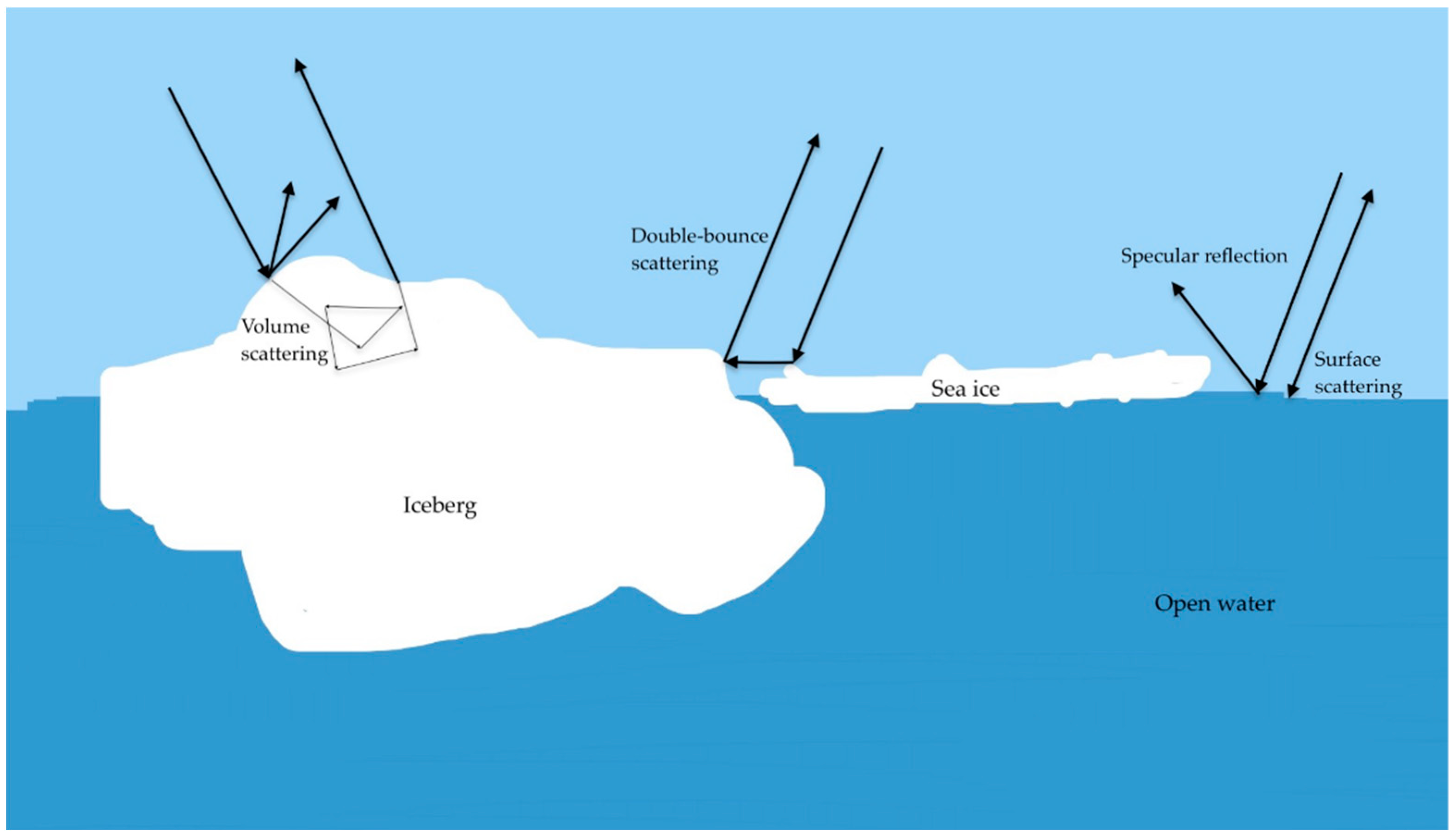
Spaceborne Observation and Iceberg Detection
2. Materials and Methods
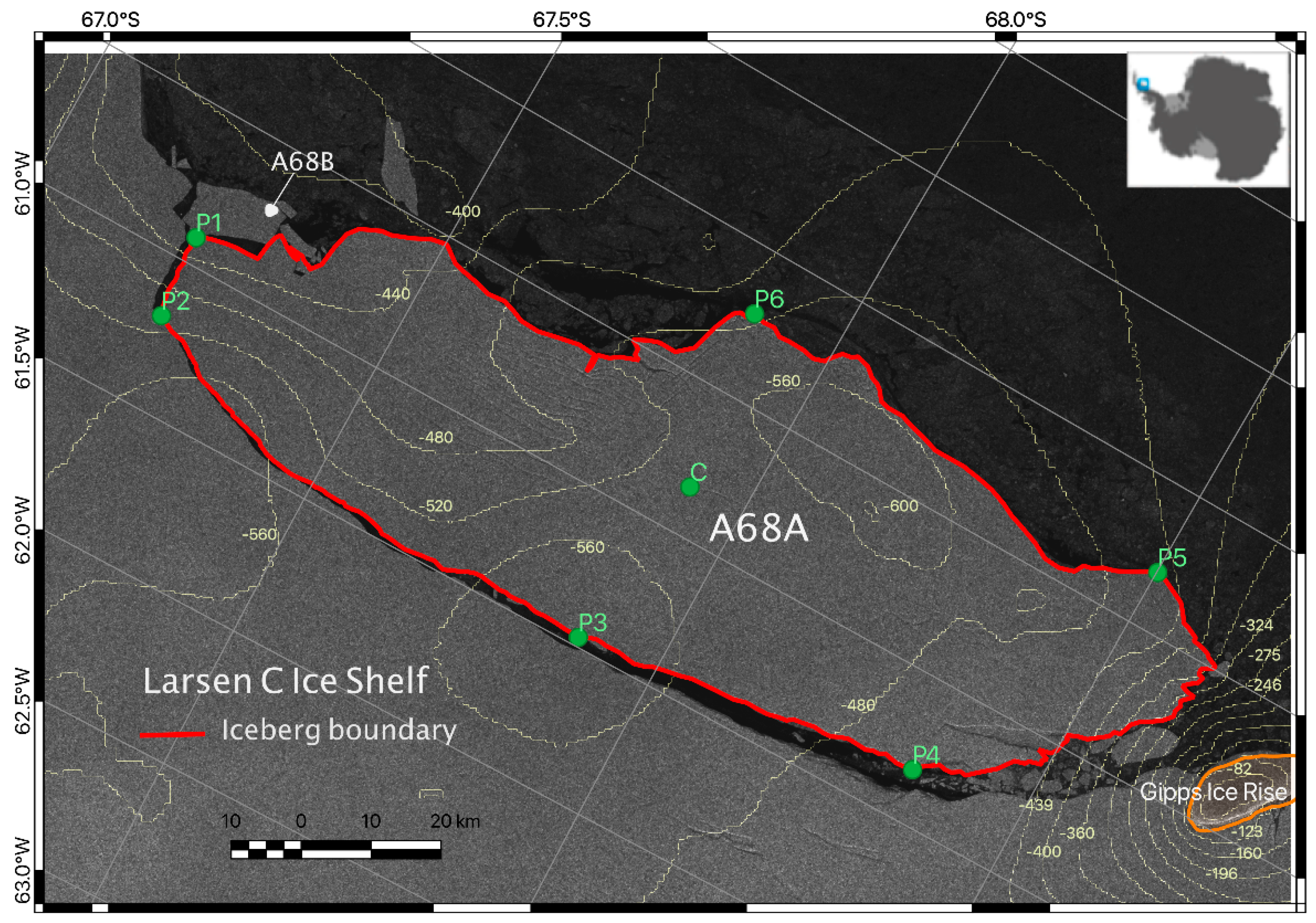
2.1. Collapse of the Larsen C Ice Shelf and Evolution of Iceberg A68
2.2. Dataset
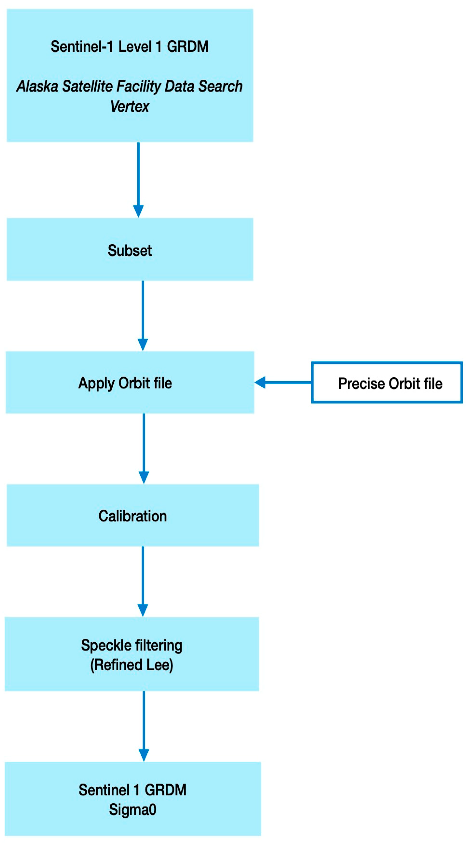
2.3. SAR Data Preprocessing Workflow
2.4. Trajectory Analysis
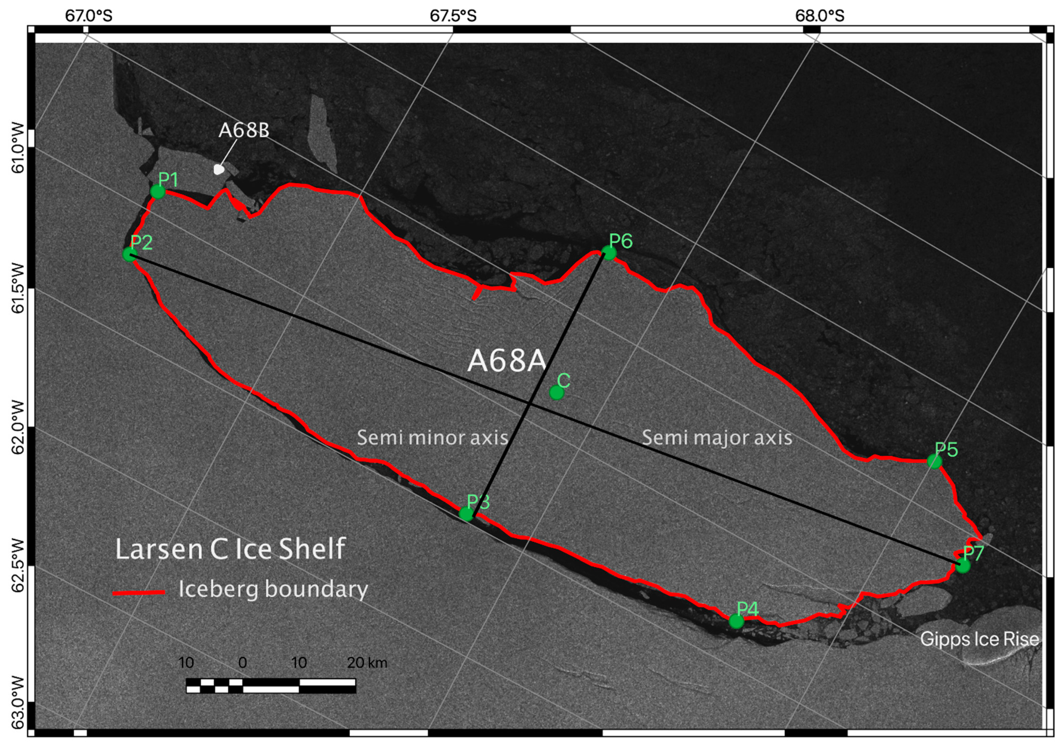
2.4.1. Ellipsoid Correction
2.4.2. Area Calculation
2.4.3. Analysis of Bathymetry on A68’s Evolution
3. Results and Discussion
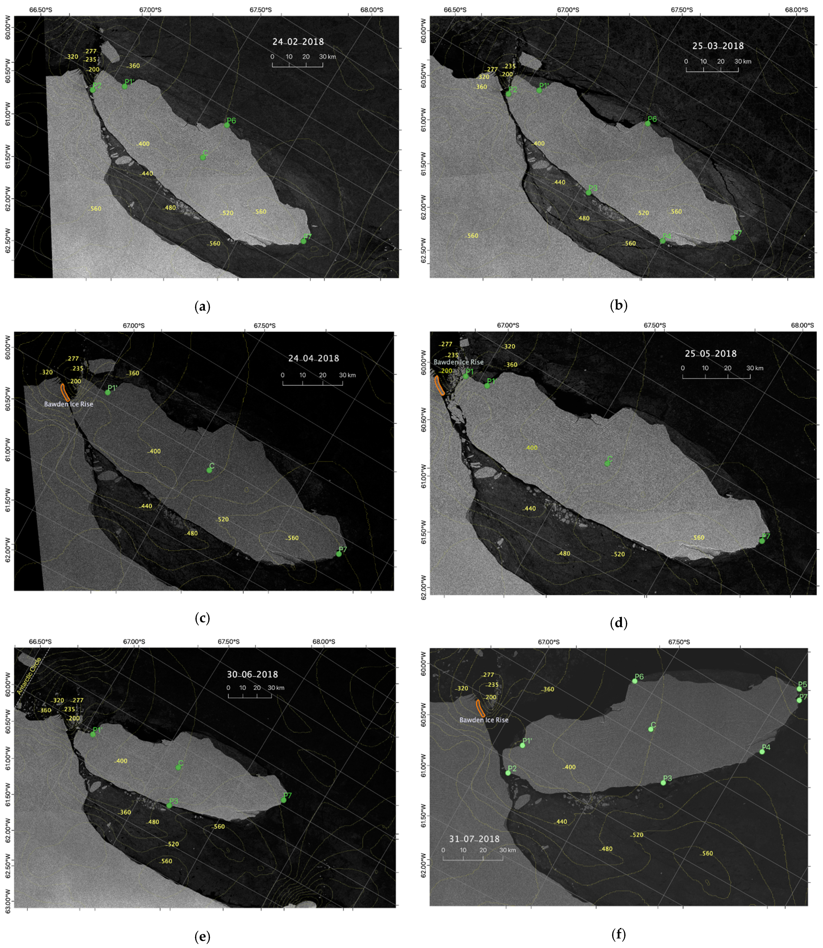
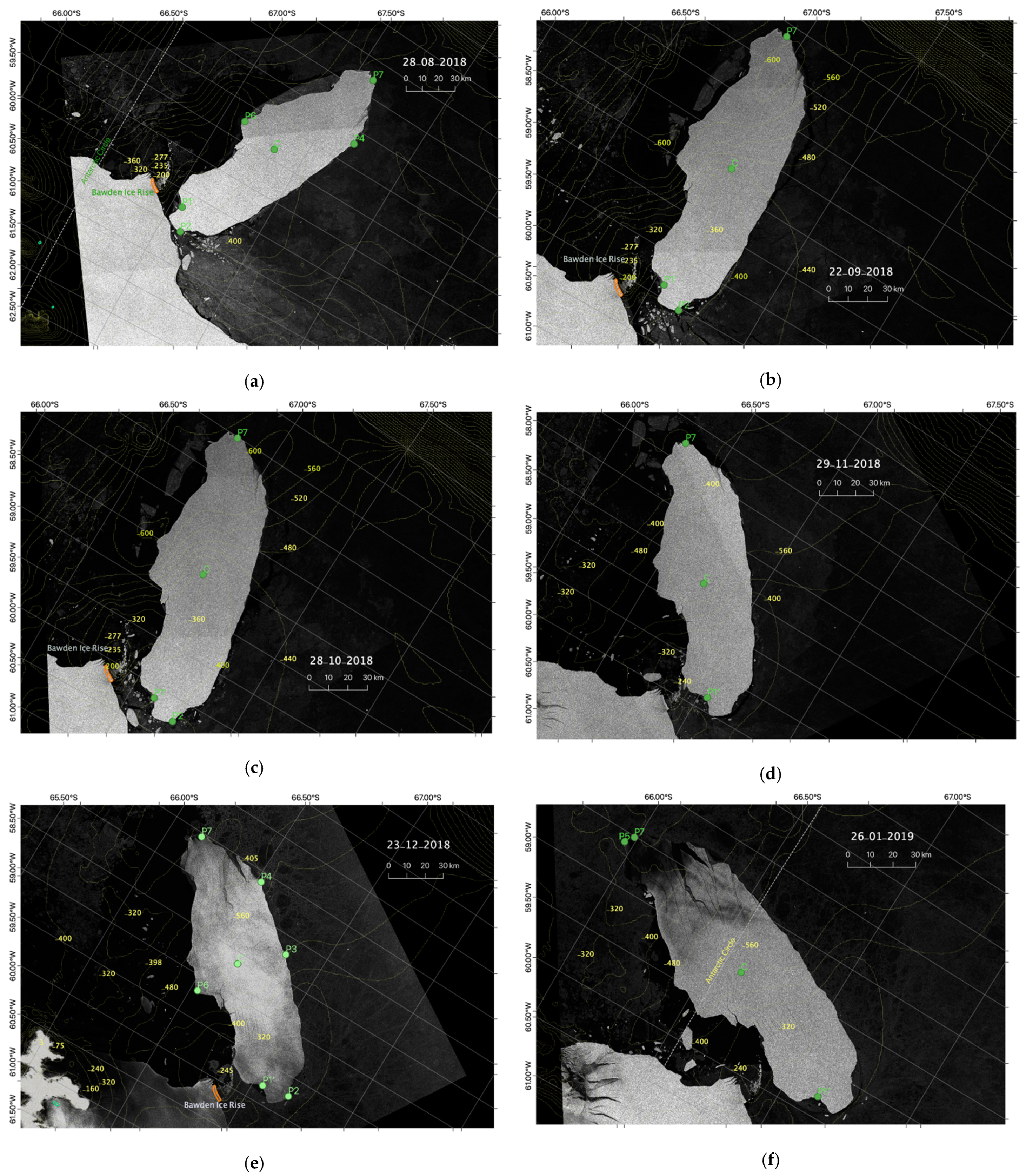
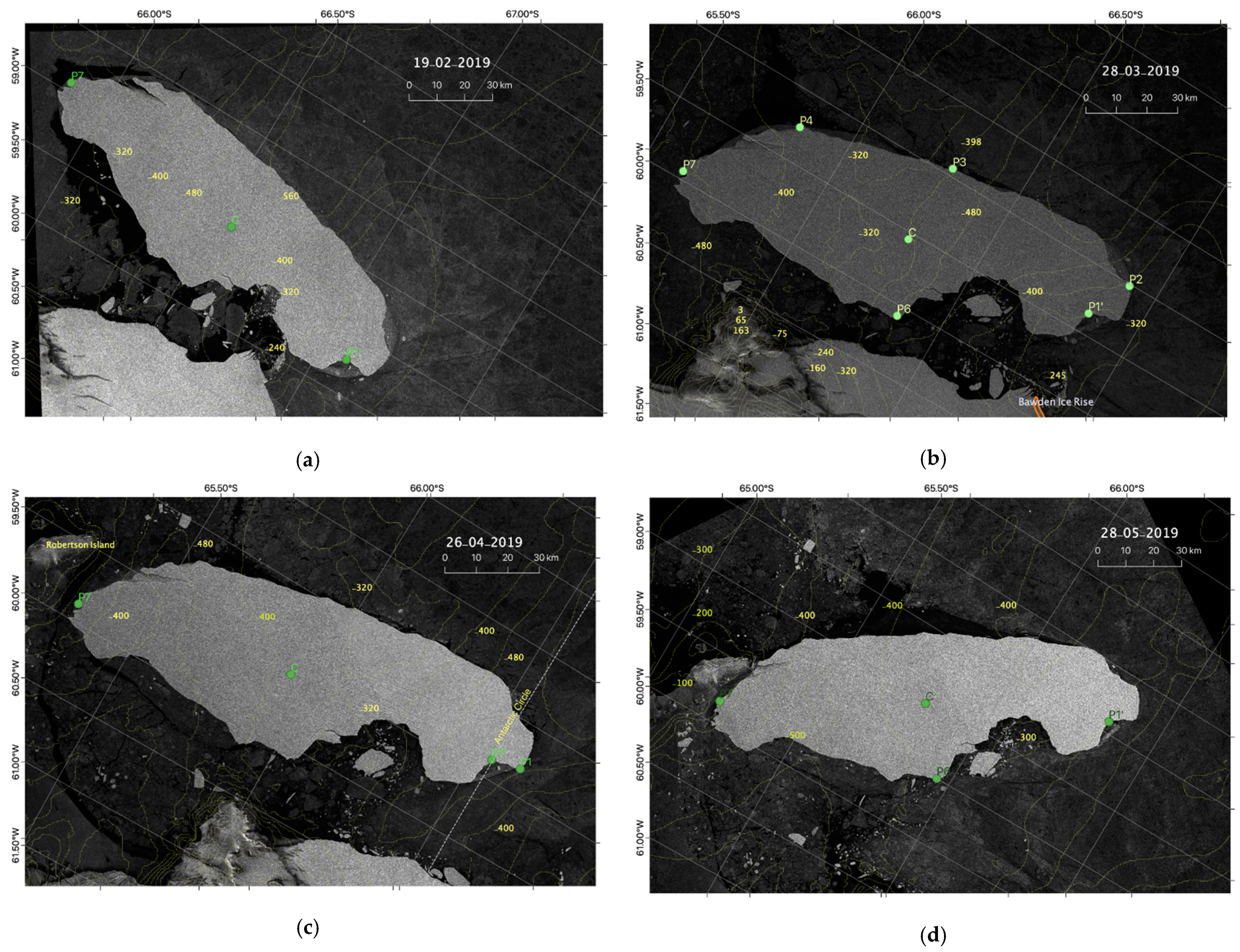
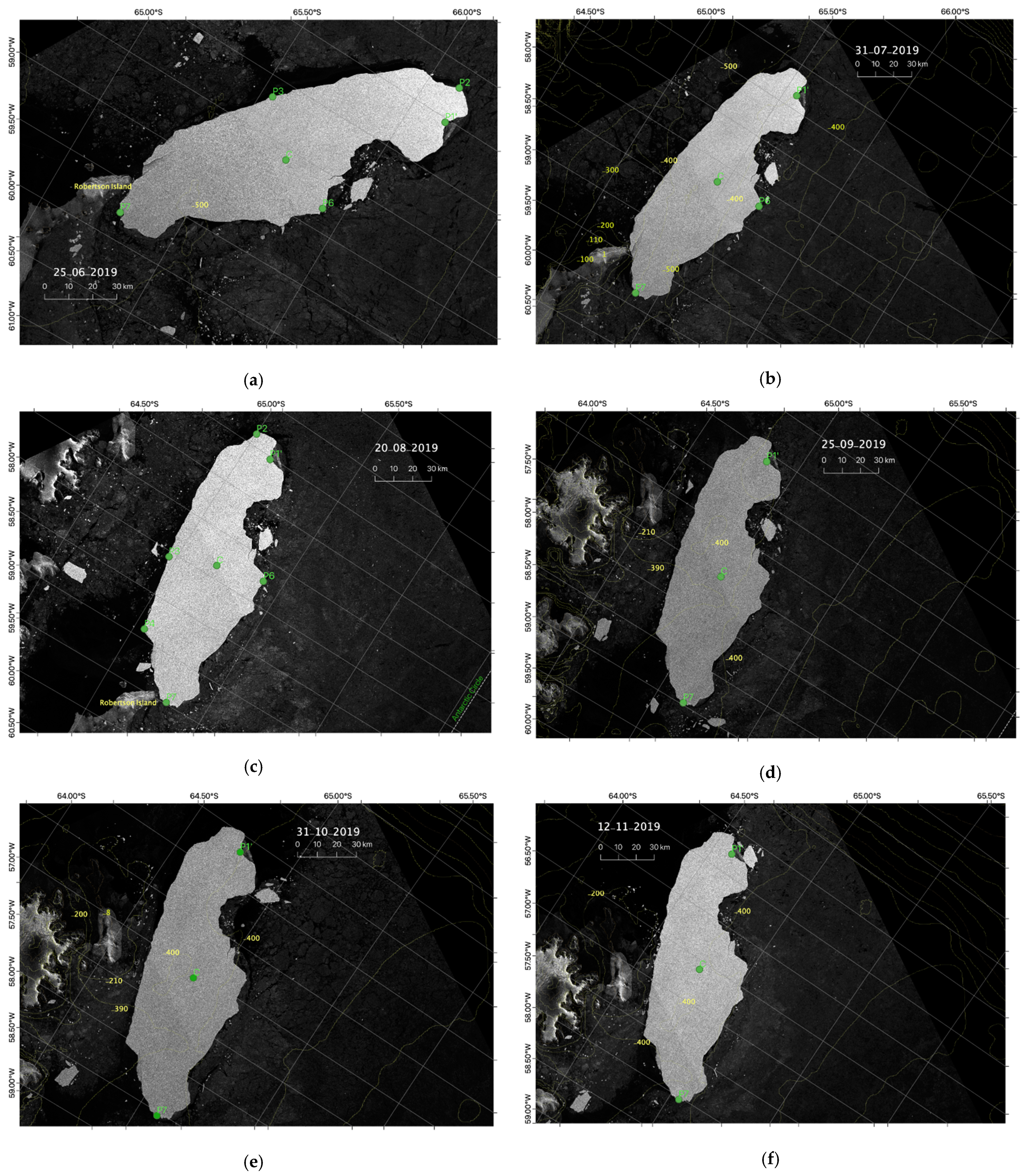
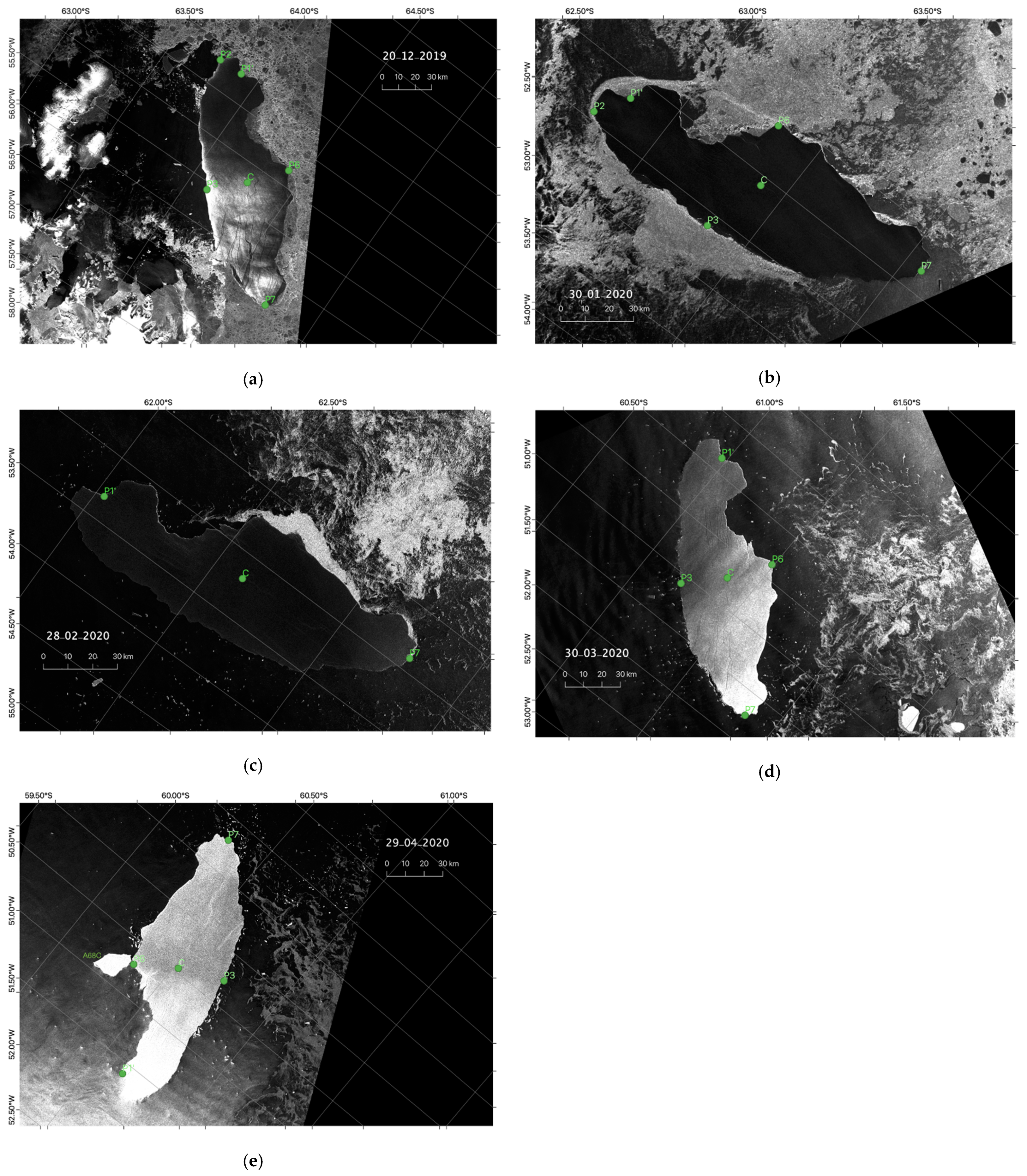
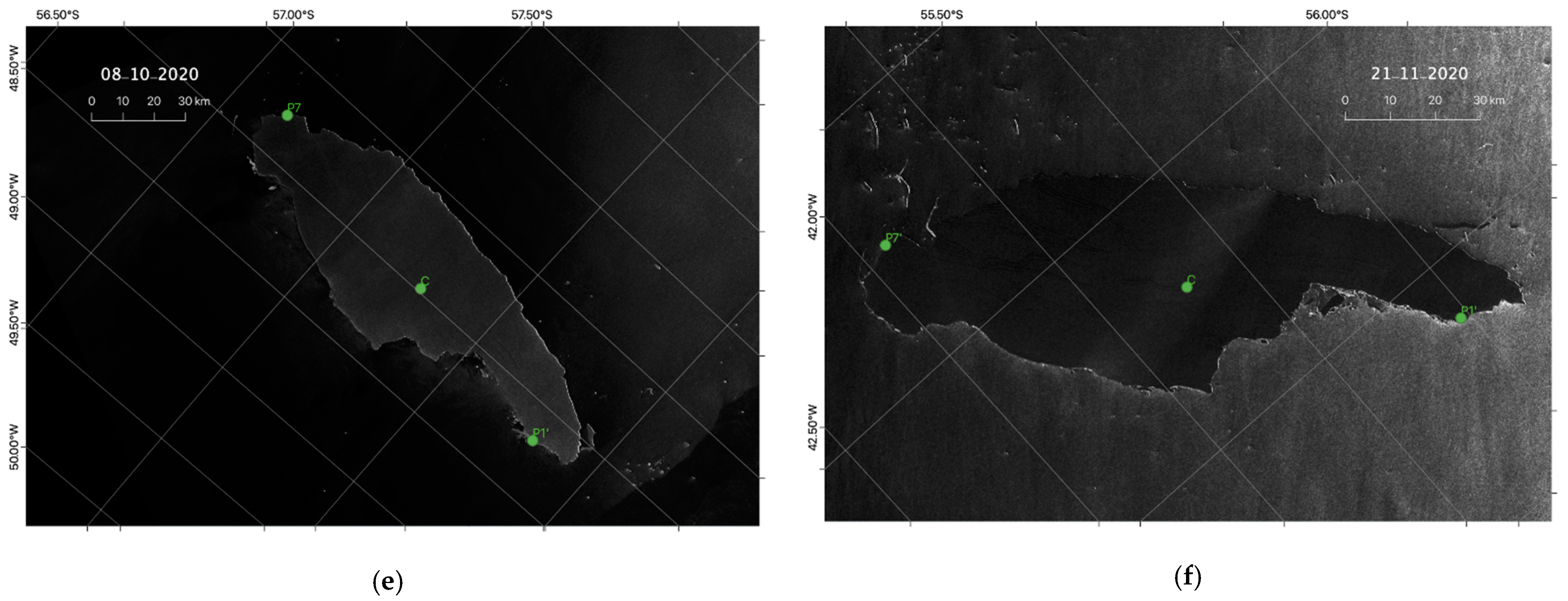
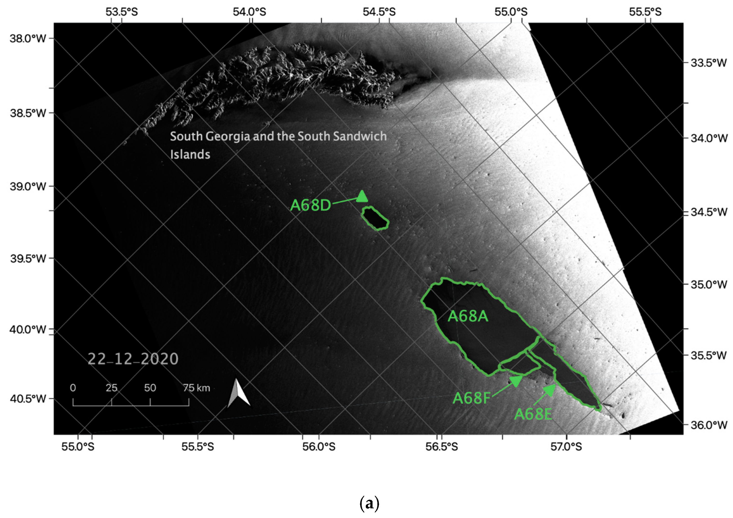
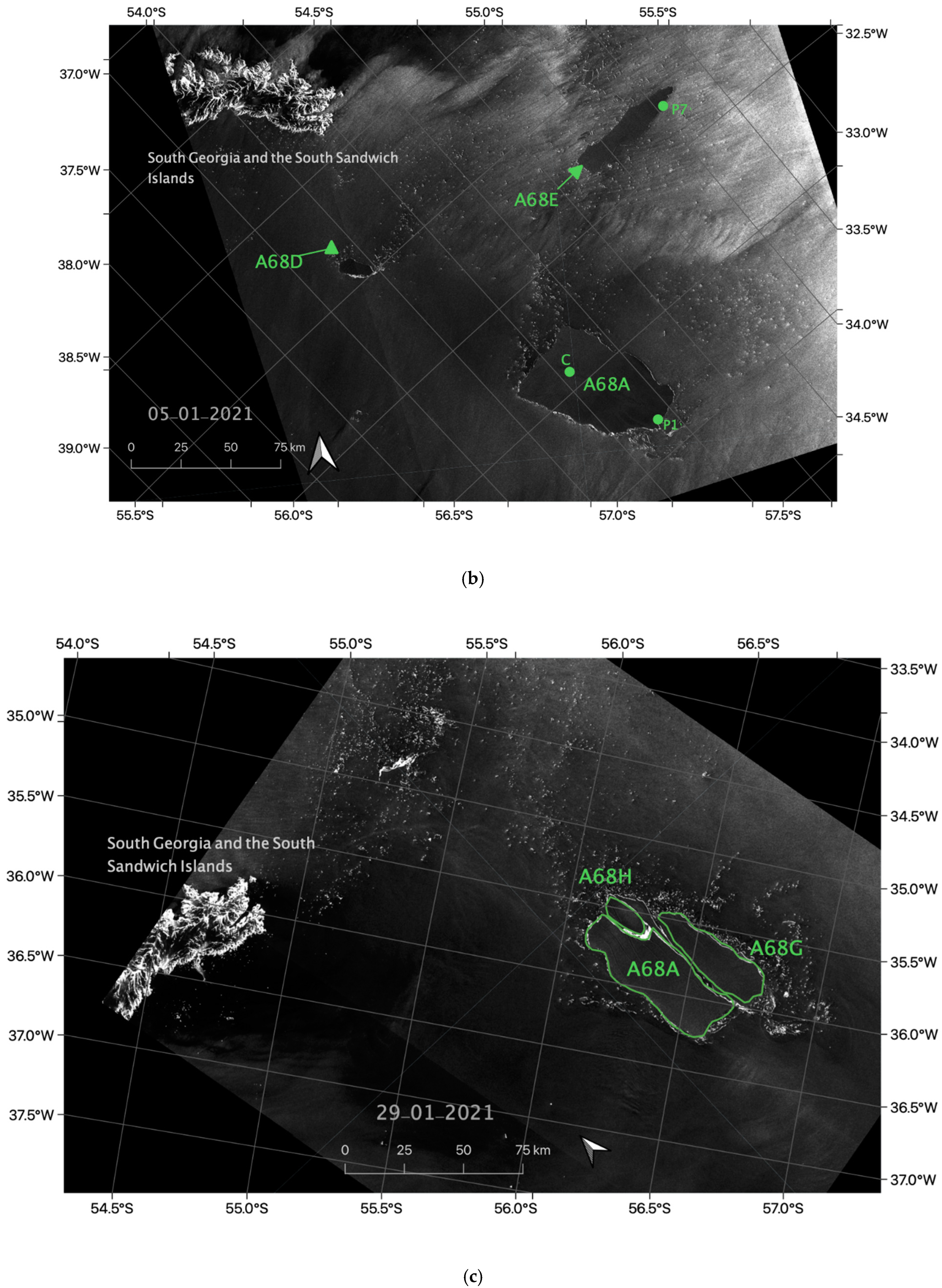
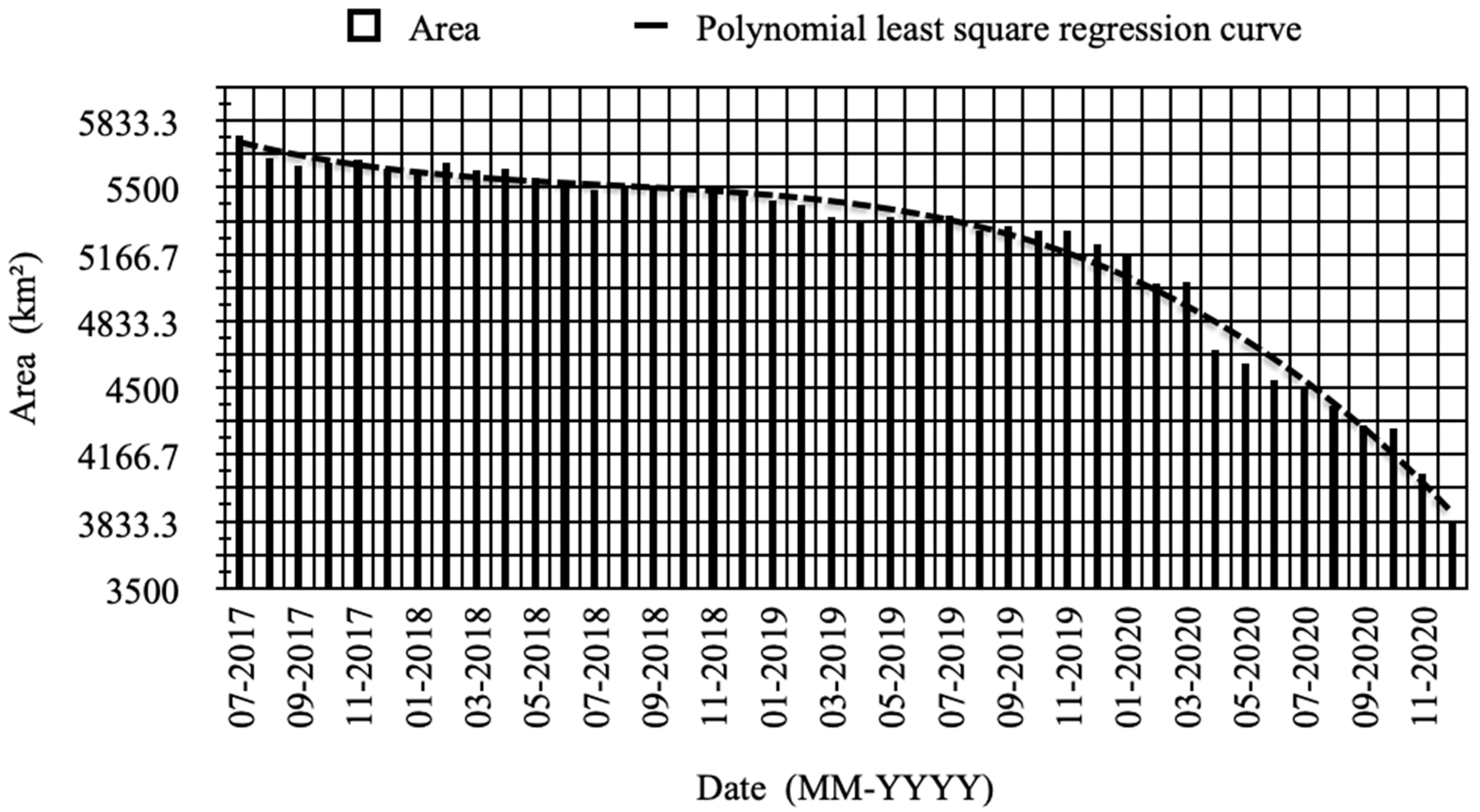
3.1. A68 Area
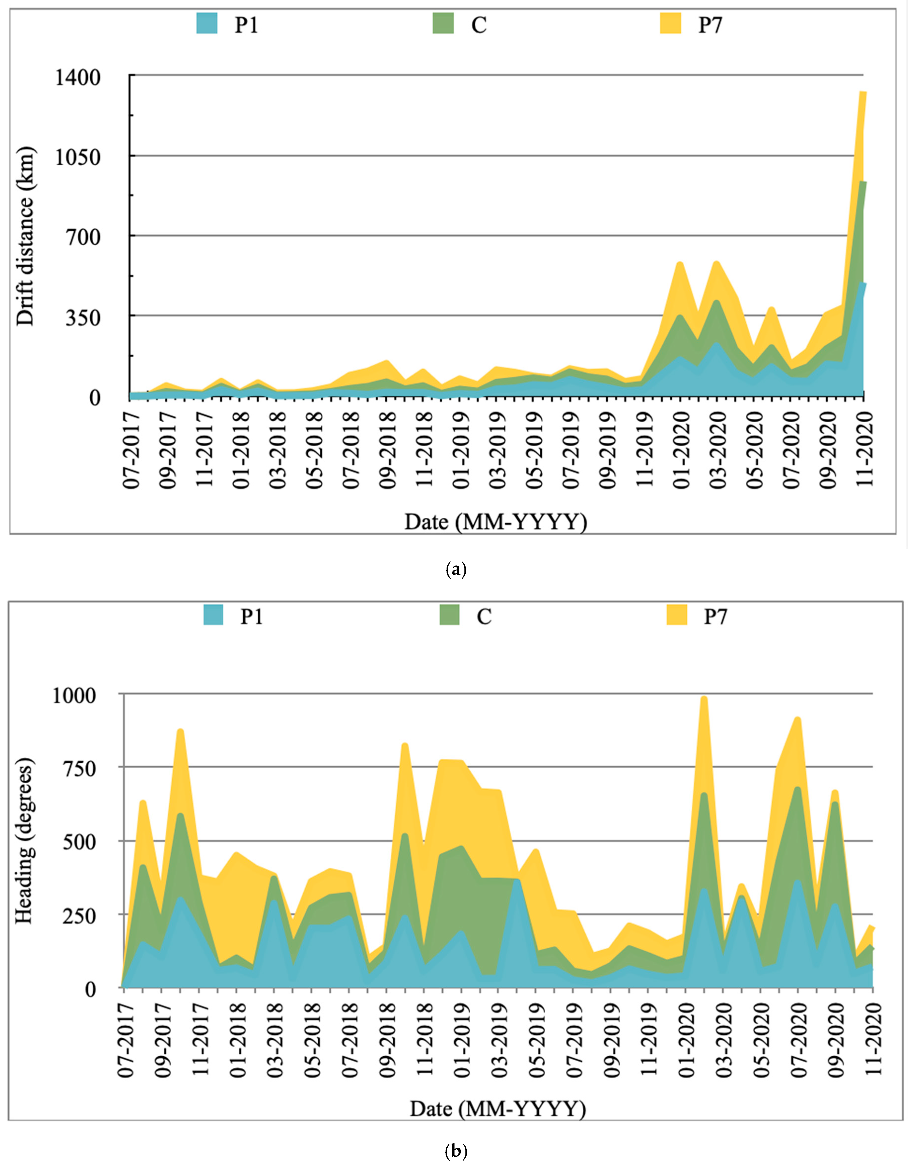
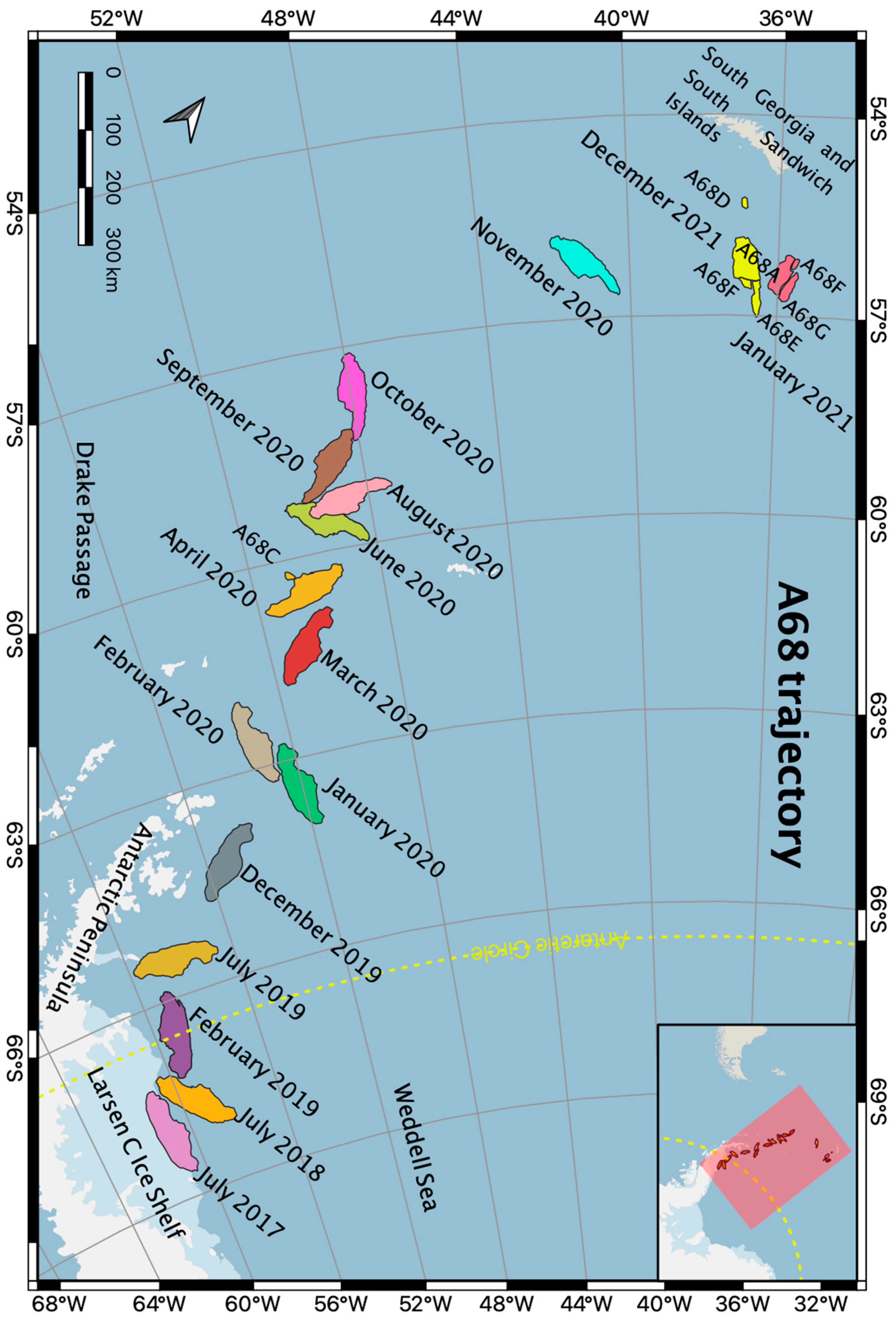
3.2. A68 Trajectory
4. Conclusions
Author Contributions
Funding
Institutional Review Board Statement
Informed Consent Statement
Data Availability Statement
Acknowledgments
Conflicts of Interest
Appendix A

| Date | Satellite/Acquisition Mode | Pass | Product |
|---|---|---|---|
| 27 July 2017 | S1-A/EW | Ascending | S1A_EW_GRDM_1SSH_20170727T002304_20170727T002404_017649_01D8BC_C976 |
| 3 August 2017 | S1-A/EW | Ascending | S1A_EW_GRDM_1SSH_20170803T001459_20170803T001559_017751_01DBC9_F634 |
| 25 September 2017 | S1-A/EW | Ascending | S1A_EW_GRDM_1SSH_20170925T002307_20170925T002407_018524_01F37A_0311 |
| 26 October 2017 | S1-A/EW | Ascending | S1A_EW_GRDM_1SSH_20171026T001502_20171026T001602_018976_020126_F936 |
| 7 November 2017 | S1-A/EW | Ascending | S1A_EW_GRDM_1SSH_20171107T001502_20171107T001602_019151_020690_D6E4 |
| 25 December 2017 | S1-A/EW | Ascending | S1A_EW_GRDM_1SSH_20171225T001500_20171225T001600_019851_021C62_4E3F |
| 25 January 2018 | S1-B/EW | Ascending | S1B_EW_GRDM_1SDH_20180125T235803_20180125T235903_009334_010C0A_D6F0 |
| 24 February 2018 | S1-A/EW | Ascending | S1A_EW_GRDM_1SSH_20180224T235845_20180224T235945_020755_023922_2621 |
| 25 March 2018 | S1-B/EW | Ascending | S1B_EW_GRDM_1SDH_20180325T001417_20180325T001517_010180_0127F5_17C4 |
| 24 April 2018 | S1-A/EW | Ascending | S1A_EW_GRDM_1SSH_20180424T001500_20180424T001600_021601_0253BE_8BC2 |
| 25 May 2018 | S1-B/EW | Ascending | S1B_EW_GRDM_1SDH_20180525T235806_20180525T235906_011084_01451D_2B57 |
| 30 June 2018 | S1-B/EW | Ascending | S1B_EW_GRDM_1SDH_20180630T235808_20180630T235908_011609_01557E_7086 |
| 31 July 2018 | S1-B/EW | Ascending | S1B_EW_GRDM_1SDH_20180731T235005_20180731T235103_012061_016359_71AA |
| 28 August 2018 | S1-B/EW | Ascending | S1B_EW_GRDM_1SDH_20180828T001425_20180828T001525_012455_016F83_4B18 |
| 22 September 2018 | S1-B/EW | Ascending | S1B_EW_GRDM_1SDH_20180922T235812_20180922T235912_012834_017B29_8D97 |
| 28 October 2018 | S1-B/EW | Ascending | S1B_EW_GRDM_1SDH_20181028T235813_20181028T235913_013359_018B4E_37AD |
| 29 November 2018 | S1-B/EW | Ascending | S1B_EW_GRDH_1SDH_20181129T075243_20181129T075343_013816_0199BA_7EEB |
| 23 December 2018 | S1-B/EW | Descending | S1B_EW_GRDH_1SDH_20181223T075243_20181223T075343_014166_01A531_6C6E |
| 26 January 2019 | S1-A/EW | Ascending | S1A_EW_GRDM_1SSH_20190126T235852_20190126T235952_025655_02D96F_A401 |
| 19 February 2019 | S1-A/EW | Ascending | S1A_EW_GRDM_1SSH_20190219T235851_20190219T235951_026005_02E5F2_4A84 |
| 28 March 2019 | S1-B/EW | Ascending | S1B_EW_GRDM_1SSH_20190328T235009_20190328T235113_015561_01D2B7_2B7C |
| 26 April 2019 | S1-A/EW | Descending | S1A_EW_GRDM_1SSH_20190426T080952_20190426T081100_026958_0308AE_2513 |
| 28 May 2019 | S1-B/EW | Descending | S1B_EW_GRDM_1SDH_20190528T075244_20190528T075344_016441_01EF2D_3039 |
| 25 June 2019 | S1-A/EW | Descending | S1A_EW_GRDM_1SSH_20190625T080955_20190625T081102_027833_032466_897E |
| 31 July 2019 | S1-A/EW | Descending | S1A_EW_GRDM_1SSH_20190731T080957_20190731T081105_028358_033457_13EA |
| 20 August 2019 | S1-B/EW | Descending | S1B_EW_GRDH_1SDH_20190820T075249_20190820T075349_017666_0213C3_F0A9 |
| 25 September 2019 | S1-B/EW | Descending | S1B_EW_GRDH_1SDH_20190925T075250_20190925T075350_018191_02240E_D460 |
| 31 October 2019 | S1-B/EW | Descending | S1B_EW_GRDH_1SDH_20191031T075250_20191031T075350_018716_02346C_B773 |
| 12 November 2019 | S1-B/EW | Descending | S1B_EW_GRDM_1SDH_20191112T075250_20191112T075350_018891_023A13_5BFE |
| 20 December 2019 | S1-A/EW | Ascending | S1A_EW_GRDM_1SSH_20191220T232735_20191220T232835_030438_037BDA_8A3B |
| 30 January 2020 | S1-B/EW | Descending | S1B_EW_GRDM_1SDH_20200130T074327_20200130T074427_020043_025ECE_BC3C |
| 28 February 2020 | S1-B/EW | Descending | S1B_EW_GRDH_1SDH_20200228T075147_20200228T075247_020466_026C71_83C0 |
| 30 March 2020 | S1-B/EW | Descending | S1B_EW_GRDM_1SDH_20200330T074327_20200330T074427_020918_027AC5_C291 |
| 29 April 2020 | S1-A/EW | Ascending | S1A_EW_GRDM_1SSH_20200429T224716_20200429T224816_032348_03BE82_E107 |
| 3 May 2020 | S1-B/EW | Ascending | S1B_EW_GRDH_1SSH_20200503T230242_20200503T230342_021423_028AB9_436B |
| 23 May 2020 | S1-A/EW | Ascending | S1A_EW_GRDM_1SSH_20200523T224717_20200523T224817_032698_03C996_8684 |
| 28 June 2020 | S1-A/EW | Ascending | S1A_EW_GRDM_1SSH_20200628T224719_20200628T224819_033223_03D95B_CEDA |
| 29 July 2020 | S1-A/EW | Ascending | S1A_EW_GRDM_1SSH_20200729T223916_20200729T224016_033675_03E727_568B |
| 28 August 2020 | S1-A/EW | Ascending | S1B_EW_GRDM_1SSH_20200828T223836_20200828T223936_023129_02BEA9_A7FD |
| 27 September 2020 | S1-A/EW | Ascending | S1A_EW_GRDM_1SSH_20200927T223919_20200927T224019_034550_040586_0FBC |
| 8 October 2020 | S1-B/EW | Descending | S1B_EW_GRDM_1SDH_20201008T074232_20201008T074336_023718_02D11F_8F67 |
| 25 November 2020 | S1-A/EW | Ascending | S1A_EW_GRDM_1SSH_20201125T215925_20201125T220025_035410_042365_957F |
| 22 December 2020 | S1-A/EW | Ascending | S1A_EW_GRDM_1SSH_20201222T071734_20201222T071834_035795_0430AC_13DF |
| 5 January 2021 | S1-A/EW | Ascending | S1A_EW_GRDM_1SSH_20210105T070105_20210105T070205_035999_0437A6_68B2 |
| 29 January 2021 | S1-A/EW | Ascending | S1A_EW_GRDM_1SSH_20210129T070125_20210129T070225_036349_0443E7_153A |
| 1 February 2021 | S1-B/EW | Ascending | S1B_EW_GRDM_1SSH_20210201T214125_20210201T214229_025418_03070C_4DBB |
References
- Copland, L.; Mueller, D.R.; Weir, L. Rapid Loss of the Ayles Ice Shelf, Ellesmere Island, Canada. Geophys. Res. Lett. 2007, 34, 21501. [Google Scholar] [CrossRef] [Green Version]
- Rignot, E.; Velicogna, I.; Van Den Broeke, M.R.; Monaghan, A.; Lenaerts, J. Acceleration of the Contribution of the Greenland and Antarctic Ice Sheets to Sea Level Rise. Geophys. Res. Lett. 2011, 38, L05503. [Google Scholar] [CrossRef] [Green Version]
- Joughin, I.; Smith, B.E.; Medley, B. Marine Ice Sheet Collapse Potentially under Way for the Thwaites Glacier Basin, West Antarctica. Science 2014, 344, 735–738. [Google Scholar] [CrossRef] [PubMed]
- Smith, K.L.; Sherman, A.D.; Shaw, T.J.; Sprintall, J. Icebergs as Unique Lagrangian Ecosystems in Polar Seas. Ann. Rev. Mar. Sci. 2013, 5, 269–287. [Google Scholar] [CrossRef] [PubMed] [Green Version]
- Vernet, M.; Smith, K.L.; Cefarelli, A.O.; Helly, J.J.; Kaufmann, R.S.; Lin, H.; Long, D.G.; Murray, A.E.; Robison, B.H.; Ruhl, H.A.; et al. Islands of Ice: Influence of Free-Drifting Antarctic Icebergs on Pelagic Marine Ecosystems. Oceanography 2012, 25, 38–39. [Google Scholar] [CrossRef]
- Stern, A.A.; Adcroft, A.; Sergienko, O. The Effects of Antarctic Iceberg Calving-Size Distribution in a Global Climate Model. J. Geophys. Res. Ocean. 2016, 121, 5773–5788. [Google Scholar] [CrossRef]
- Bigg, G.R.; Wadley, M.R.; Stevens, D.P.; Johnson, J.A. Modelling the Dynamics and Thermodynamics of Icebergs. Cold Reg. Sci. Technol. 1997, 26, 113–135. [Google Scholar] [CrossRef] [Green Version]
- Death, R.; Siegert, M.J.; Bigg, G.R.; Wadley, M.R. Modelling Iceberg Trajectories, Sedimentation Rates and Meltwater Input to the Ocean from the Eurasian Ice Sheet at the Last Glacial Maximum. Palaeogeogr. Palaeoclimatol. Palaeoecol. 2006, 236, 135–150. [Google Scholar] [CrossRef]
- Martin, T.; Adcroft, A. Parameterizing the Fresh-Water Flux from Land Ice to Ocean with Interactive Icebergs in a Coupled Climate Model. Ocean Model. 2010, 34, 111–124. [Google Scholar] [CrossRef]
- Jongma, J.I.; Driesschaert, E.; Fichefet, T.; Goosse, H.; Renssen, H. The Effect of Dynamic–Thermodynamic Icebergs on the Southern Ocean Climate in a Three-Dimensional Model. Ocean Model. 2009, 26, 104–113. [Google Scholar] [CrossRef]
- Daley, C.; Veitch, B. Iceberg Evolution Modelling: A Background Study; NRC Publications Archive: Vancover, BC, Canada, 2000; pp. 20–53. [Google Scholar]
- Smith, S.D.; Banke, E.G. The Influence of Winds, Currents and Towing Forces on the Drift of Icebergs. Cold Reg. Sci. Technol. 1983, 6, 241–255. [Google Scholar] [CrossRef]
- Lichey, C.; Hellmer, H. Modeling Giant Iceberg Drift under the Influence of Sea Ice in the Weddell Sea. J. Glaciol. 2001, 47, 452–460. [Google Scholar] [CrossRef] [Green Version]
- Keghouche, I.; Bertino, L.; Lisæter, K.A. Parameterization of an Iceberg Drift Model in the Barents Sea. J. Atmos. Ocean. Technol. 2009, 26, 2216–2227. [Google Scholar] [CrossRef] [Green Version]
- Garrett, C.; Middleton, J.; Hazen, M.; Majaess, F. Tidal Currents and Eddy Statistics From Iceberg Trajectories off Labrador. Science 1985, 227, 1333–1335. [Google Scholar] [CrossRef] [PubMed]
- Smith, S.D. Hindcasting Iceberg Drift Using Current Profiles and Winds. Cold Reg. Sci. Technol. 1993, 22, 33–45. [Google Scholar] [CrossRef]
- Wagner, T.J.W.; Dell, R.W.; Eisenman, I. An Analytical Model of Iceberg Drift. J. Phys. Oceanogr. 2016, 47, 1605–1616. [Google Scholar] [CrossRef]
- Han, H.; Lee, S.; Kim, J.-I.; Kim, S.H.; Kim, H. Changes in a Giant Iceberg Created from the Collapse of the Larsen C Ice Shelf, Antarctic Peninsula, Derived from Sentinel-1 and CryoSat-2 Data. Remote Sens. 2019, 11, 404. [Google Scholar] [CrossRef] [Green Version]
- Parmiggiani, F.; Moctezuma-Flores, M.; Guerrieri, L.; Battagliere, M.L. SAR Analysis of the Larsen-C A-68 Iceberg Displacements. Int. J. Remote Sens. 2018, 39, 5850–5858. [Google Scholar] [CrossRef]
- Wesche, C.; Dierking, W. Estimating Iceberg Paths Using a Wind-Driven Drift Model. Cold Reg. Sci. Technol. 2016, 125, 31–39. [Google Scholar] [CrossRef]
- Yulmetov, R.; Marchenko, A.; Løset, S. Iceberg and Sea Ice Drift Tracking and Analysis off North-East Greenland. Ocean Eng. 2016, 123, 223–237. [Google Scholar] [CrossRef]
- Frost, A.; Ressel, R.; Lehner, S. Automated Iceberg Detection Using High-Resolution X-Band SAR Images. Can. J. Remote Sens. 2016, 42, 354–366. [Google Scholar] [CrossRef] [Green Version]
- Oliver, C.; Quegan, S. Understanding Synthetic Aperture Radar Images, 2nd ed.; SciTech Publishing Inc.: Boston, MA, USA, 2004; ISBN 1-891121-31-6. [Google Scholar]
- Tao, D.; Anfinsen, S.N.; Brekke, C. Robust CFAR Detector Based on Truncated Statistics in Multiple-Target Situations. IEEE Trans. Geosci. Remote Sens. 2016, 54, 117–134. [Google Scholar] [CrossRef]
- Al-Hussaini, E.K.; Al-Hussaini, E.K.; Ibrahim, B.M. Comparison of Adaptive Cell-Averaging Detectors for Multiple-Target Situations. IEE Proc. F Commun. Radar Signal Process. 1986, 133, 217–223. [Google Scholar] [CrossRef]
- Barkat, M.; Himonas, S.D.; Varshney, P.K. CFAR Detection for Multiple Target Situations. IEE Proc. Part F Commun. Radar Signal Process. 1989, 136, 193–209. [Google Scholar] [CrossRef]
- Crisp, D.J. The State-of-the-Art in Ship Detection in Synthetic Aperture Radar Imagery; DSTO Information Sciences Laboratory: Edinburgh, Australia, 2004. [Google Scholar]
- Silva, T.A.M.; Bigg, G.R. Computer-Based Identification and Tracking of Antarctic Icebergs in SAR Images. Remote Sens. Environ. 2005, 94, 287–297. [Google Scholar] [CrossRef]
- Wesche, C.; Dierking, W. Iceberg Signatures and Detection in SAR Images in Two Test Regions of the Weddell Sea, Antarctica. J. Glaciol. 2012, 58, 325–339. [Google Scholar] [CrossRef] [Green Version]
- Williams, R.N.; Rees, W.G.; Young, N.W. A Technique for the Identification and Analysis of Icebergs in Synthetic Aperture Radar Images of Antarctica. Int. J. Remote Sens. 1999, 20, 3183–3199. [Google Scholar] [CrossRef] [Green Version]
- Willis, C.J.; Macklin, J.T.; Partington, K.C.; Teleki, K.A.; Rees, W.G.; Williams, R.G. Iceberg Detection Using ERS-1 Synthetic Aperture Radar. Int. J. Remote Sens. 1996, 17, 1777–1795. [Google Scholar] [CrossRef]
- Young, N.W.; Turner, D.; Hyland, G.; Williams, R.N. Near-Coastal Iceberg Distributions in East Antarctica, 50–145° E. Ann. Glaciol. 1998, 27, 68–74. [Google Scholar] [CrossRef] [Green Version]
- Langley, K.; Hamran, S.-E.; Hogda, K.A.; Storvold, R.; Brandt, O.; Hagen, J.O.; Kohler, J. Use of C-Band Ground Penetrating Radar to Determine Backscatter Sources within Glaciers. IEEE Trans. Geosci. Remote Sens. 2007, 45, 1236–1246. [Google Scholar] [CrossRef]
- Rignot, E.; Echelmeyer, K.; Krabill, W. Penetration Depth of Interferometric Synthetic-Aperture Radar Signals in Snow and Ice. Geophys. Res. Lett. 2001, 28, 3501–3504. [Google Scholar] [CrossRef] [Green Version]
- Akbari, V.; Brekke, C. Iceberg Detection in Open and Ice-Infested Waters Using C-Band Polarimetric Synthetic Aperture Radar. IEEE Trans. Geosci. Remote Sens. 2018, 56, 407–421. [Google Scholar] [CrossRef]
- Gill, R.S. Operational Detection of Sea Ice Edges and Icebergs Using SAR. Can. J. Remote Sens. 2001, 27, 411–432. [Google Scholar] [CrossRef]
- Power, D.; Youden, J.; Lane, K.; Randell, C.; Flett, D. Iceberg Detection Capabilities of RADARSAT Synthetic Aperture Radar. Can. J. Remote Sens. 2001, 27, 476–486. [Google Scholar] [CrossRef]
- Marino, A.; Dierking, W.; Wesche, C. A Depolarization Ratio Anomaly Detector to Identify Icebergs in Sea Ice Using Dual-Polarization SAR Images. IEEE Trans. Geosci. Remote Sens. 2016, 54, 5602–5615. [Google Scholar] [CrossRef] [Green Version]
- Kim, J.-W.; Kim, D.; Kim, S.-H.; Hwang, B.-J. Iceberg Detection Using Full-Polarimetric RADARSAT-2 SAR Data in West Antarctica. In Proceedings of the 2011 3rd International Asia-Pacific Conference on Synthetic Aperture Radar (APSAR), Seoul, Republic of Korea, 26–30 September 2011; pp. 1–4. [Google Scholar]
- Dierking, W.; Wesche, C. C-Band Radar Polarimetry—Useful for Detection of Icebergs in Sea Ice? IEEE Trans. Geosci. Remote Sens. 2014, 52, 25–37. [Google Scholar] [CrossRef]
- Crocker, R.I.; Maslanik, J.A.; Adler, J.J.; Palo, S.E.; Herzfeld, U.C.; Emery, W.J. A Sensor Package for Ice Surface Observations Using Small Unmanned Aircraft Systems. IEEE Trans. Geosci. Remote Sens. 2012, 50, 1033–1047. [Google Scholar] [CrossRef]
- Benn, D.I.; Åström, J.A. Calving Glaciers and Ice Shelves. Adv. Phys. X 2018, 3, 1048–1076. [Google Scholar] [CrossRef] [Green Version]
- National Snow & Ice Data Center. National Snow and Ice Data Center—Advancing Knowledge of Earth’s Frozen Regions. Available online: https://nsidc.org/ (accessed on 14 September 2021).
- Scambos, T.A.; Bohlander, J.A.; Shuman, C.A.; Skvarca, P. Glacier Acceleration and Thinning after Ice Shelf Collapse in the Larsen B Embayment, Antarctica. Geophys. Res. Lett. 2004, 31, L18402. [Google Scholar] [CrossRef] [Green Version]
- European Space Agency. Keeping an Eye on Wilkins Ice Shelf. Available online: https://www.esa.int/Applications/Observing_the_Earth/Keeping_an_eye_on_Wilkins_Ice_Shelf (accessed on 14 September 2021).
- Rott, H.; Skvarca, P.; Nagler, T. Rapid Collapse of Northern Larsen Ice Shelf, Antarctica. Science 1996, 271, 788–792. [Google Scholar] [CrossRef]
- Rignot, E.; Jacobs, S.; Mouginot, J.; Scheuchl, B. Ice-Shelf Melting around Antarctica. Science 2013, 341, 266–270. [Google Scholar] [CrossRef] [PubMed] [Green Version]
- Massom, R.A.; Scambos, T.A.; Bennetts, L.G.; Reid, P.; Squire, V.A.; Stammerjohn, S.E. Antarctic Ice Shelf Disintegration Triggered by Sea Ice Loss and Ocean Swell. Nature 2018, 558, 383–389. [Google Scholar] [CrossRef] [PubMed]
- Davies, B. The Larsen C Ice Shelf Growing Rift Antarctic Peninsula Ice Shelves. Available online: https://www.antarcticglaciers.org/2017/06/larsen-c-ice-rift/ (accessed on 15 November 2022).
- Loff, S. Rift in Antarctica’s Larsen C Ice Shelf. Available online: https://www.nasa.gov/image-feature/rift-in-antarcticas-larsen-c-ice-shelf (accessed on 15 November 2022).
- Schannwell, C.; Cornford, S.; Pollard, D.; Barrand, N.E. Dynamic Response of Antarctic Peninsula Ice Sheet to Potential Collapse of Larsen C and George VI Ice Shelves. Cryosphere 2018, 12, 2307–2326. [Google Scholar] [CrossRef] [Green Version]
- Booth, A.; Luckman, A.; White, J.; Pearce, E.; Cornford, S.; Kulessa, B.; Brisbourne, A.; Hubbard, B. Mechanical Response of Larsen C Ice Shelf Following the A68 Calving Event: Observations from Field-Based Geophysical Measurements. In Proceedings of the EGU General Assembly Conference, Vienna, Austria, 4–13 April 2018; p. 10049. [Google Scholar]
- Arndt, J.E.; Schenke, H.W.; Jakobsson, M.; Nitsche, F.O.; Buys, G.; Goleby, B.; Rebesco, M.; Bohoyo, F.; Hong, J.; Black, J.; et al. The International Bathymetric Chart of the Southern Ocean (IBCSO) Version 1.0—A New Bathymetric Compilation Covering Circum-Antarctic Waters. Geophys. Res. Lett. 2013, 40, 3111–3117. [Google Scholar] [CrossRef] [Green Version]
- Thomas, R.H. The Dynamics of Marine Ice Sheets. J. Glaciol. 1979, 24, 167–177. [Google Scholar] [CrossRef] [Green Version]
- Walter, F.; O’Neel, S.; McNamara, D.; Pfeffer, W.T.; Bassis, J.N.; Fricker, H.A. Iceberg Calving during Transition from Grounded to Floating Ice: Columbia Glacier, Alaska. Geophys. Res. Lett. 2010, 37, L15501. [Google Scholar] [CrossRef] [Green Version]
- Ren, D.; Leslie, L.M.; Lynch, M.J. Verification of Model Simulated Mass Balance, Flow Fields and Tabular Calving Events of the Antarctic Ice Sheet against Remotely Sensed Observations. Clim. Dyn. 2013, 40, 2617–2636. [Google Scholar] [CrossRef] [Green Version]
- Liu, H.; Li, X.M.; Guo, H. The Dynamic Processes of Sea Ice on the East Coast of Antarctica—A Case Study Based on Spaceborne Synthetic Aperture Radar Data from TerraSAR-X. IEEE J. Sel. Top. Appl. Earth Obs. Remote Sens. 2016, 9, 1187–1198. [Google Scholar] [CrossRef]
- Ganopolski, A.; Rahmstorf, S. Rapid Changes of Glacial Climate Simulated in a Coupled Climate Model. Nature 2001, 409, 153–158. [Google Scholar] [CrossRef]
- Hemming, S.R. Heinrich Events: Massive Late Pleistocene Detritus Layers of the North Atlantic and Their Global Climate Imprint. Rev. Geophys. 2004, 42, RG1005. [Google Scholar] [CrossRef] [Green Version]
- Macayeal, D.R.; Okal, M.H.; Thom, J.E.; Brunt, K.M.; Kim, Y.-J.; Bliss, A.K.; Macayeal, D.R.; Okal, M.H.; Thom, J.E.; Brunt, K.M.; et al. Tabular Iceberg Collisions within the Coastal Regime. J. Glaciol. 2008, 54, 371–386. [Google Scholar] [CrossRef] [Green Version]


Disclaimer/Publisher’s Note: The statements, opinions and data contained in all publications are solely those of the individual author(s) and contributor(s) and not of MDPI and/or the editor(s). MDPI and/or the editor(s) disclaim responsibility for any injury to people or property resulting from any ideas, methods, instructions or products referred to in the content. |
© 2023 by the authors. Licensee MDPI, Basel, Switzerland. This article is an open access article distributed under the terms and conditions of the Creative Commons Attribution (CC BY) license (https://creativecommons.org/licenses/by/4.0/).
Share and Cite
Singh, S.; Kumar, S.; Kumar, N. Evolution of Iceberg A68 since Its Inception from the Collapse of Antarctica’s Larsen C Ice Shelf Using Sentinel-1 SAR Data. Sustainability 2023, 15, 3757. https://doi.org/10.3390/su15043757
Singh S, Kumar S, Kumar N. Evolution of Iceberg A68 since Its Inception from the Collapse of Antarctica’s Larsen C Ice Shelf Using Sentinel-1 SAR Data. Sustainability. 2023; 15(4):3757. https://doi.org/10.3390/su15043757
Chicago/Turabian StyleSingh, Shivangini, Shashi Kumar, and Navneet Kumar. 2023. "Evolution of Iceberg A68 since Its Inception from the Collapse of Antarctica’s Larsen C Ice Shelf Using Sentinel-1 SAR Data" Sustainability 15, no. 4: 3757. https://doi.org/10.3390/su15043757
APA StyleSingh, S., Kumar, S., & Kumar, N. (2023). Evolution of Iceberg A68 since Its Inception from the Collapse of Antarctica’s Larsen C Ice Shelf Using Sentinel-1 SAR Data. Sustainability, 15(4), 3757. https://doi.org/10.3390/su15043757