Application of Deep Learning to Enforce Environmental Noise Regulation in an Urban Setting

Abstract

Reducing environmental noise in urban settings, i.e., unwanted or harmful outdoor sounds produced by human activity, has become an important issue in recent years. Most countries have established regulations that set maximum permitted noise levels. However, enforcing these regulations effectively remains challenging as it requires active monitoring networks and audio analysis performed by trained specialists. The manual evaluation of the audio recordings is laborious, time-consuming, and inefficient since many audios exceeding the noise level threshold do not correspond to a sound event considered by the regulation. To address this challenge, this work proposes a computational pipeline to assist specialists in detecting noise sources in the built environment that do not comply with the Chilean noise regulation. The system incorporates a deep neural model following a pre-trained audio neural network architecture transferred to a dataset compiled from public sources and recordings in Valdivia, Chile. The target dataset follows a customized taxonomy of urban sound events. The system also uses a public API so potential users can post audio files to obtain a prediction matrix reporting the presence of noise sources contributing to environmental noise pollution. Experiments using recordings from two continuous noise monitoring stations showed that the amount of data to be inspected by the specialist is decreased by 97% when the deep-learning tools are used. Therefore, this system efficiently assists trained experts in enforcing noise legislation through machine-assisted environmental noise monitoring.

1. Introduction

The growth of cities has led to an increase in noise levels, which affects people’s health at different levels. This phenomenon has been analyzed in different cities around the world, such as New York [1], Guangzhou [2], Sambalpur [3], and other cities in China [4] and Europe [5], where there is increasing concern about this kind of pollution. In this way, reducing noise pollution in the built environment aligns with some of the UN’s Sustainable Development Goals [6], especially Goals 3 (“ensure healthy lives and promote well-being for all at all ages”) and 11 (“make cities and human settlements inclusive, safe, resilient and sustainable”). Thus, many countries aim to promote sustainable land-use planning and management and promote sustainable industrial activities.

In order to create high-quality urban settings in response to societal, environmental, and economic concerns, such as noise pollution, it is crucial to consider the built environment’s quality [7,8]. Environmental acoustics addresses urban design for sustainable urban environments by relating mainly to several sub-areas of the earth sciences, life sciences, and engineering. Thus, environmental acoustics is a broad, interdisciplinary topic in which acousticians must collaborate with experts from different fields. Even though environmental acoustics includes all of the sounds in the environment, either natural or artificial, the main concern is those “unwanted sounds” that adversely affect people’s physiological and psychological well-being. These sounds make up environmental noise. In this sense, environmental noise is the unwanted or harmful outdoor sound created by human activity, such as noise emitted through transport, road traffic, rail traffic, air traffic, and industrial activity [9].

Environmental noise created by artificial sources is not new. Humans are susceptible to sound, especially at night, when the background noise is significantly lower than during the day. Although several examples of environmental noise can be dated back to cities in ancient Greece and Rome, we may set the origin of modern environmental noise to the industrial revolution. This transition from an agrarian and handicraft economy to one dominated by industry and machine manufacturing resulted in technological changes that introduced novel ways of working and living and fundamentally transformed society, particularly in cities. These changes made possible the vastly increased use of natural resources and the mass production of manufactured goods. This process also resulted in populations moving from rural to urban centers, making for larger cities with greater population densities. Therefore, the noise became more intense, and the population exposed to noise increased as well.

On the other hand, the introduction of affordable automobiles at the beginning of the 20th century made cars available to middle-class urban residents. This fact resulted in the construction and expansion of new roads and a massive increase in road traffic flows, which became a significant source of environmental noise in big cities.

There are many different ways to measure and evaluate environmental noise, each typically resulting in a different noise measure, descriptor, or scale [10]. From these measures and descriptors, criteria have been developed to decide on the acceptable noise levels for different activities.

A critical issue regarding environmental noise is the existence of noise regulations. In general, most countries have elaborated their legislation based on setting the maximum permitted levels in different zones and times of the day. The zones are defined by the local authorities and are related to the use of land, so lower limits are imposed in areas where the use is residential, while higher limits are set for exclusive industrial zones. Some regulations also include limits for rural zones requiring special treatment due to their lower background noise. Lower limits are defined for the night as well to prevent sleep disturbance. Usually, the maximum permitted levels are corrected according to the background noise, the presence of pure tones, and impulsive noise sources.

Real-time noise mapping is currently used in several countries, based on noise-monitoring networks that collect the noise data continuously and transmit it to a data center for further processing. Many of these monitoring networks are public, and people can access information from the internet. Dynamic noise maps are helpful for noise-sensitive areas and buildings, especially in the vicinity of airports, highways, and other primary-noise sources. This information is helpful for urban design in modern cities [11]. Additionally, continuous monitoring stations are widely used as a part of mitigation plans to monitor excessive construction and entertainment noises in the built environment.

However, the amount of data collected from a noise-monitoring network could be thousands of audio files to be analyzed manually. A trained specialist should carefully listen to each audio file individually to identify and discriminate the presence of prohibited noise sources and levels exceeded by restricted sources from the natural sounds of the environment [12]. This fact leads to a slow and time-consuming procedure. As a result, it is necessary to optimize the data analysis, which can be achieved by using the current advances in machine learning technology.

Machine learning (ML) technology has evolved rapidly and has found applications in different fields in recent years. Deep learning (DL) is a branch in the field of ML that is focused on training deep artificial neural networks (ANNs) to solve complex pattern-recognition problems [13]. ANN are bio-inspired mathematical models formed by concatenating layers of simple processing elements called artificial neurons. In practice, the deeper a model is, i.e., the more layers it contains, the more flexibility it has to fit the training data. The remarkable results obtained by DL models have positioned them as the de-facto choice for perception-related problems such as computer vision [14], speech recognition [15], and natural language processing [16]. One crucial challenge is that the deeper the models, the more labeled data are needed to train them effectively. Hence, large, good-quality datasets are critical.

The use of ML techniques in urban noise has been introduced previously. To estimate the energy-equivalent A-weighted sound-pressure level descriptor (LAeq), Torija and Ruiz [17] investigated three ML regression techniques that are considered very robust in tackling non-linear problems. They also experimented with two feature-selection methods and a data-reduction method. Their study resulted in a proposal of various strategies based on data collection and accuracy requirements. In another study [18], traffic-noise annoyance models were obtained by applying ML techniques. The study showed that the ML approach, in particular an ANN, performed better than traditional statistical models in producing accurate predictions of the impact of transportation noise in an urban context.

Alvares-Sanches et al. [19] recently used audio recordings obtained in walking surveys carried out in Southampton, UK, combined with ML, to predict noise levels across the entire city. They claimed that their technique could be suitable for noise data collected by individuals, from noise-monitoring networks, or by structured surveys. In a more recent study, Fredianelli et al. [20] proposed an ML application for road-traffic noise mapping. They created a system that complies with the standards of the CNOSSOS-EU noise-assessment model [21] by utilizing inexpensive video cameras and vehicle recognition and a counting procedure using ML approaches. The technique was successfully used in a small Italian city to create noise maps and determine the population exposed to road-traffic noise.

Tasks associated with audio data have had greater visibility thanks to challenges such as DCASE (https://dcase.community/, accessed on 1 November 2022). Since its first edition in 2013, this challenge has promoted the resolution of tasks such as acoustic-scene classification (ASC), sound-event detection (SED), and audio tagging by implementing deep learning algorithms. Audio tagging is an essential task of audio-pattern recognition, which aims to predict the presence or absence of labeled sound sources in an audio file. Consequently, implementing deep neural network models for audio tagging has yielded promising results in the last few years [22,23,24,25,26].

Bianco et al. [27] comprehensively reviewed the recent advances in ML, including DL, in the field of acoustics. They reported that ML-based methods exhibited better performance than conventional signal-processing techniques despite the fact that they require a large amount of data for testing and training.

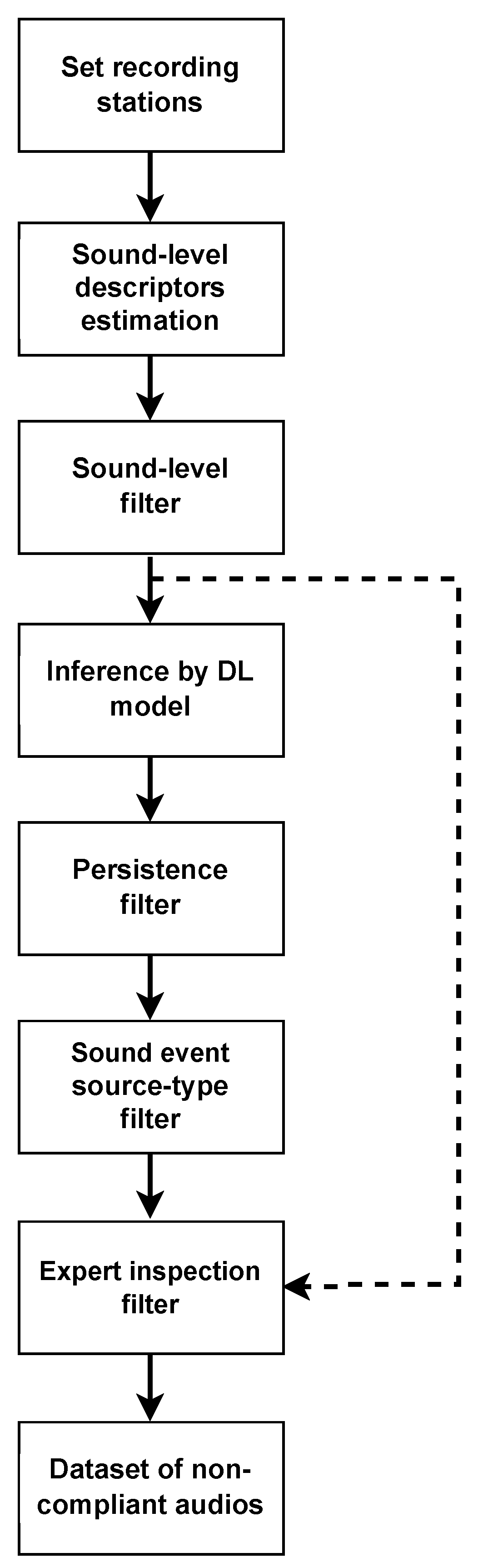
The Institutes of Acoustics and Informatics at the College of Engineering Sciences of the University Austral of Chile have been working on a joint project titled “Integrated System for the Analysis of Environmental Sound Sources: FuSA System”. The project is funded through a grant from the Chilean Science Ministry. The project aims to create a machine-learning-based system that automatically recognizes sound sources in audio files recorded in the built environment to assist in their analysis.

In this paper, we present the results of using the tools developed in the FuSA project to analyze the environmental noise recorded at two points in the city of Valdivia, applying the current Chilean environmental noise regulation. The study reported here contributes to efficiently assisting trained experts in enforcing noise legislation through machine-assisted environmental noise monitoring.

2. Materials and Methods

2.1. Chilean Environmental Noise Regulations

Environmental noise emissions are regulated in Chile by law DS No 38/11 of the Ministry of the Environment. This regulation, enacted in 2011, aims to protect the community’s well-being by establishing maximum allowable noise levels generated by the sources covered by the regulation. The limits established by the regulation are based on the land uses described in the local Territorial Planning Guidelines in force where the receiver is located. These noise limits are lower at night. Article 7 of the regulation establishes that the corrected A-weighted sound pressure levels (NPC) obtained from the emission of a noise source measured at the receiver location cannot exceed the values shown in

Table 1. Corrected maximum permissible sound pressure levels (NPC) in dB(A) (MMA, 2011).

	From 7 a.m. to 9 p.m.	From 9 p.m. to 7 a.m.
Zone I	55 dB(A)	45 dB(A)
Zone II	60 dB(A)	45 dB(A)
Zone III	65 dB(A)	50 dB(A)
Zone IV	70 dB(A)	70 dB(A)

.

In Table 1, the zones located within the urban limits are divided into four types: (1) Zone I, which encompasses exclusively residential areas and/or public or green spaces; (2) Zone II, which includes all of Zone I as well as commercial and business areas; (3) Zone III, which includes all of Zone II plus productive and/or infrastructure activities; and (4) Zone IV, which is restricted to heavy industrial areas. For rural areas outside the urban limit, Article 9 of the regulation establishes that the NPC value must be the lower of either (a) the background noise level + 10 dB(A) or (b) the NPC for Zone II of Table 1.

The regulation also establishes the requirements for performing the measurements either outdoors or indoors. In the latter condition, additional corrections must be applied to account for the presence of doors, windows, or openings in the walls or roof that may affect the propagation of noise indoors.

Three 1-min measurements are carried out at each test point when applying the regulation. The highest value between the measured LAeq and the maximum LAeq minus 5 dB(A) is chosen for each measurement. Thus, the resulting LAeq at a location before any correction is the arithmetic average of the three results.

2.2. Deep Learning Models for Acoustic Event Classification

The authors of [26] presented the pretrained audio neural network (PANN), a deep neural network model for audio tagging that outperformed previous systems in the literature. PANN was trained using Google AudioSet [28], a dataset with more than 2 million 10-s audio clips collected from YouTube and classified into 632 categories. The architecture of PANN consists mainly of convolutional layers, i.e., processing layers with neurons organized as convolutional filters [29]. Two filter columns run in parallel within PANN. The first one consists of 2D convolutional layers operating on the input’s log-scaled mel-spectrogram (LogMel). In contrast, the second consists of 1D convolutional layers operating on the waveform to form its time-frequency representation called WaveGram. The information extracted from the LogMel and WaveGram representations is concatenated and further processed to return the model’s predictions.

Perhaps more interesting than its architecture is that PANN was designed as a baseline for general audio-related problems. Deep neural networks trained with a large corpus of data can be used to solve a more specific (but intrinsically related) problem through a methodology called transfer learning (TL) [30]. In TL, a target dataset representing a particular task that may have a different class taxonomy concerning the source dataset is used to adapt the parameters of the final layers of the original model. This process is called fine-tuning. Using TL, a very deep model can be effectively trained even with a relatively small target dataset, given that the source dataset is sufficiently general.

The FuSA system incorporates a deep neural model following PANN’s architecture that was transferred to a dataset of urban sound events compiled from public sources [31] and recordings captured by FuSA in the city of Valdivia, Chile. The target dataset follows a customized taxonomy shown in

Table 2. Urban sound event taxonomy used in the FuSA system.

Categories			Subcategories
Humans	talking	screaming	crowd	others
Music	music
Animals	dog	bird	others
Environment	rain	wind	waterfall	thunder	others
Mechanical	impact	cutting	explosion	drilling	others
Vehicles			bus	helicopter
	motorcycle	car	and	and	others
			truck	plane
Alerts	siren	alarm	horn	bell	others

. The system has an API in which users post an audio file through an HTTP request and receive a matrix representing the presence of the predominant sound source for each 5-s window of the audio file.

Figure 1 shows how to obtain a prediction from the FuSA system through an HTTP request. Listing 1 corresponds to the HTTP query requesting the FuSA system’s prediction. The parameter “model” allows the user to choose which prediction model to use, and the parameter “file” corresponds to the audio file to be processed. This file can be in .wav format or any other audio format. The parameter “X-Api-Key” corresponds to the security key of the guest users. Listing 2 is the response of the FuSA system in a JSON format. The response displays the model and its version, the date the prediction was made, and the categories of sounds detected. Further instructions on consulting this public API can be found in the FuSA system documentation (https://api.labacam.org/docs, accessed on 1 January 2023). Figure 2 shows a colormap visualization of the response from the FuSA system for a 1-min audio recording. The system returns class probabilities (vertical axis) for every 5-s segment of the recording (horizontal axis), i.e., a prediction matrix. The probabilities add up to one in the vertical axis, and the darker the color, the greater the probability. This result allows the experts to quickly assess the dynamics of the acoustic environment in terms of the presence of its loudest sound events.

In this work, the FuSA system was used to classify sound events within audio files recorded in Valdivia following the methodology presented in the next section.

2.3. Environmental-Noise Data Collection

Audio recordings and acoustic data were obtained from a continuous noise monitoring station (Capta by Absentia). The station is suitable for outdoor installation with a 3-inch waterproof windscreen and complies with IEC 61672-3 [32]. Its dynamic range is 25–110 dB(A), with a sampling frequency of 40 kHz, and it can store acoustic data in A-, C-, and Z-weighting. The station was calibrated to 94 dB(A) every time before each use. For this particular study, one station was used for two locations in different periods. The station uses a lithium battery to operate continuously for one to two days. However, since one week was the minimum required measurement, the station was connected to an external power supply for uninterrupted operation. The station also contains a SIM card with mobile data for uploading acoustic and audio data to the manufacturer’s web platform. This characteristic allowed access to the data without needing to access the station physically.

As shown in Figure 3, the first location of the station was in the backyard of a two-story house, which is located in a passageway on Vicente Perez Rosales Street. The property adjacent to the north of the receiving point showed earthmoving activities and a workshop that included machinery such as a backhoe and power saws. An ice factory was located on the west side of the site. Both activities generated detectable noise levels at the receptor during the daytime. Continuous measurements were recorded for two weeks.

The monitoring station was installed in a second location corresponding to a four-story residential apartment complex’s backyard (see Figure 4). The northern property adjacent to the complex had a shed and trucks belonging to a city cleaning and landscaping company, which generated noise throughout the week, including weekends. Trucks passing and heavy object movements were identified as the primary-noise sources. The monitoring station collected data for one week.

At both measuring points, 1-min audio recordings and daily reports of sound pressure levels were obtained to calculate the A-weighted equivalent continuous-sound-pressure levels (LAeq, 1 min).

2.4. Noise Regulation Compliance Assisted by DL Models

This section describes the methodology used to analyze the audio files recorded by the noise monitoring stations and verify compliance with Chilean noise regulations with the assistance of the urban sound tagging model provided by the FuSA system. Figure 5 summarizes the proposed methodology (straight arrows) and a trained specialist’s conventional procedure (dashed arrows). In this figure, the rectangles that contain filters represent states or tasks used to discard data from the pipeline. In what follows, each of the steps is described.

• Set up recording stations: The stations are set up as described in the previous section.
• Estimate sound pressure level (SPL) descriptors: The stations estimate the A-weighted Lmin, Lmax, and Leq for every 1-min segment coming from the continuous recording stream. The values of these SPL descriptors are uploaded to a database as a backup.
• SPL filter: The calibrated waveform of the 1-min segments that surpass a specified Leq threshold are saved in WAV format and uploaded to a database for further analysis. The threshold was set depending on the maximum permissible level (MPL) of the zone in which the station was located, as established by the regulation [33]. In this particular case, the land use is Zone III, according to the local territorial planning guidelines. Therefore, MPL is 65 dB(A) in the daytime and 50 dB(A) at night (see Table 1). A safe margin of 10 dBA was also considered, so the final thresholds were set to 55 dB(A) for daytime and 40 dB(A) at night.
• Inference by DL model: The 1-min audio recordings that surpassed the established sound-level limits are evaluated with the urban audio tagging model through the FuSA system API. The prediction obtained for a given audio is a matrix P, with $\dim \left(P\right)=(12\times 27)$, where the element $p_{ij}$ represents the probability of the i-th 5-s segment corresponding to the j-th urban sound event from the FuSA taxonomy. (A code example showing how to obtain and visualize DL predictions can be found at https://fusa-project.github.io/demo_sustainability/, accessed on 2 February 2023.).
• Persistence filter: 1-min audio recordings that do not comply with

  $$\frac{1}{12}\sum _{j=1}^{12}\mathrm{I}(p_{ij}\ge T)\ge 0.85,$$

  (1)

  for at least one sound-event class i are discarded from further analysis. The indicator function $\mathrm{I}(·)$ in Equation (1) is one if its argument is true and zero otherwise. The hyperparameter $T\in [0,1]$ represents the detection threshold for the model predictions. We study the influence of T in the next section. In summary, this filter discards audio recordings that only have transient (short-time) or low-probability sound events, according to the model predictions.
• Sound event source-type filter:

  Table 3. Sources of the FuSA taxonomy applicable to the Chilean noise regulation [33].

  Sources	Permitted Activities According to Land Use
  Human	Recreational activities and services
  Music	Recreational and commercial activities
  Mechanical	Productive and service activities

  describes the sound-events to which Chilean noise regulations are applicable. In this step, 1-min audio recordings with strong and persistent sound events that do not fall into these categories are discarded from further analysis.
• Expert inspection filter: The final subset of 1-min audio segments selected by the previous filters are reviewed by trained specialists to confirm the presence of urban sound events predicted by the neural network model.

3. Results

Table 4. Number of 1-min audio segments at different stages of the proposed pipeline.

Pipeline Stage	Minutes
Before SPL filter	30,240
After SPL filter	115
After persistence filter	28
After source-type filter	3
After expert inspection filter	2

summarizes the results from the audio reduction pipeline described in Section 2.4. The two monitoring stations recorded 30,240 min during their two-week and one-week operation periods. From this dataset, only 115 min were flagged as surpassing the established sound pressure level, and their corresponding waveforms were uploaded to a database. The FuSA system was then used to obtain class predictions for the 115-min subset. This subset was further reduced to 28 min after applying the persistence filter, i.e., only 28 of the 1-min audio segments contain strong and uninterrupted sound events. In this case, a detection threshold $T=0.5$ was used. The distribution of sound events at this stage of the pipeline is given in

Table 5. Category distribution of those 1-min audio segments that passed the persistence filter.

Classification	Minutes
Mechanical/digging	1
Mechanical/others	2
Environmental/rain	17
Animal/dog	8

. The last automatic filter selected three 1-min audios, which contain sound events originating from sources where the Chilean noise regulation applies. The detailed metadata of these audios are shown in

Table 6. Metadata of the three 1-min audio segments that passed all of the automatic filters. Segment 1654224726 is a false positive according to the expert’s inspection.

ID	Prediction	Leq, dB(A)	Date	Time	Location
1653409372	Mechanical/digging	73.2	24 May 2022	16:21:52	Point 1
1654224726	Mechanical/other	50.9	3 June 2022	02:52:06	Point 1
1655826106	Mechanical/other	67.9	21 June 2022	15:42:46	Point 2

.

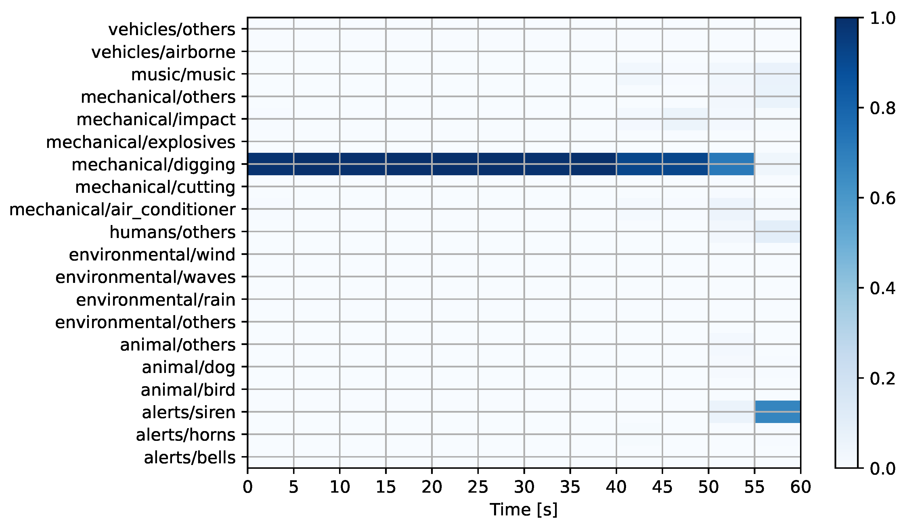
Figure 6, Figure 7 and Figure 8 show the prediction matrices corresponding to the automatically detected regulation-offending audio candidates from Table 6. For the first audio (see Figure 6), the system predicts a mechanical sound event related to digging activities. This sound event has a high probability, except during the last five seconds of the recording. The accuracy of this prediction was later confirmed upon inspection by experts. 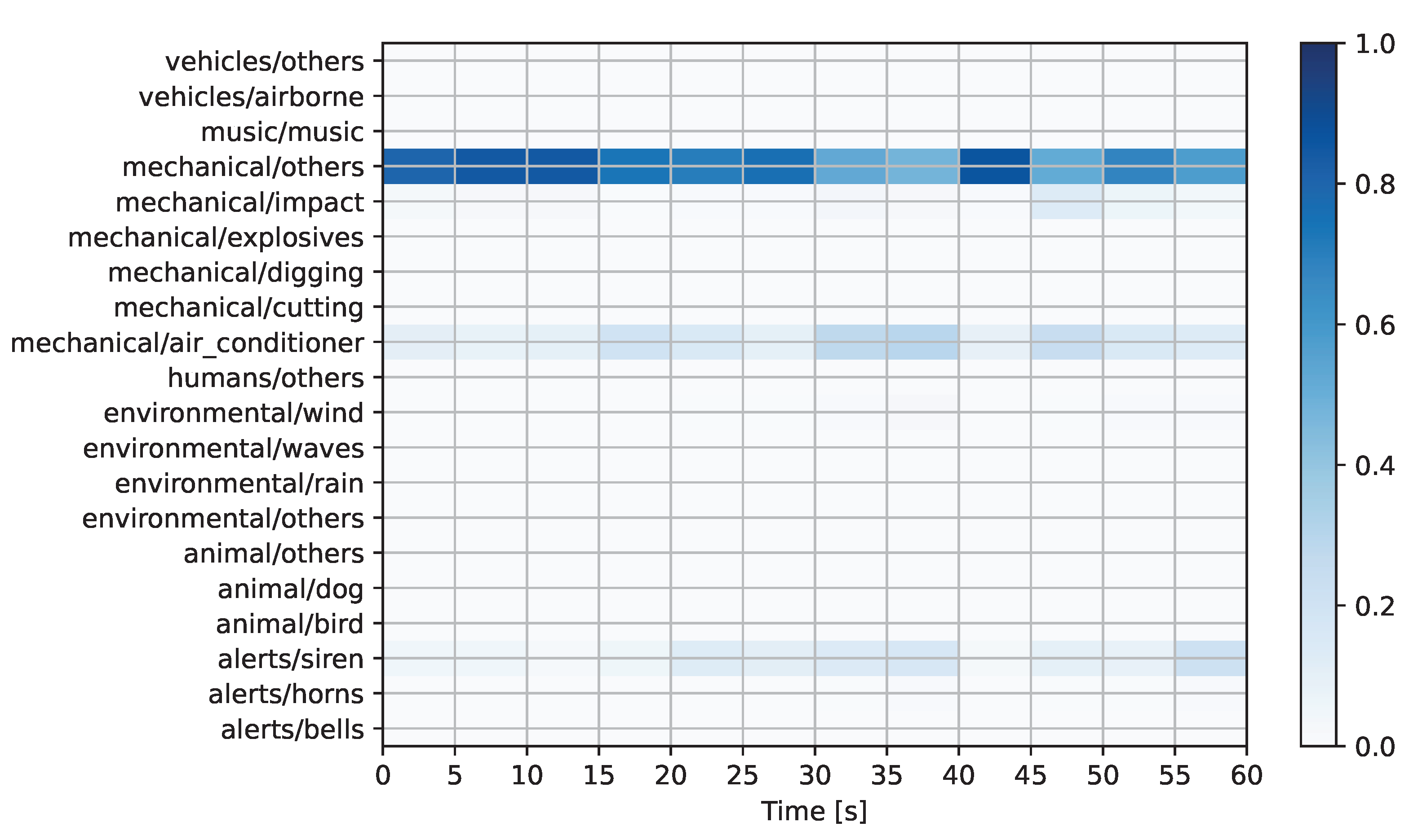For the second audio (see Figure 7), the system predicts a mechanical sound in the “others” category, with minor contributions from the air conditioner and siren classes. Later inspection by experts revealed that the prediction was incorrect as the only discernible events in the recording are of environmental origin (wind and rain). 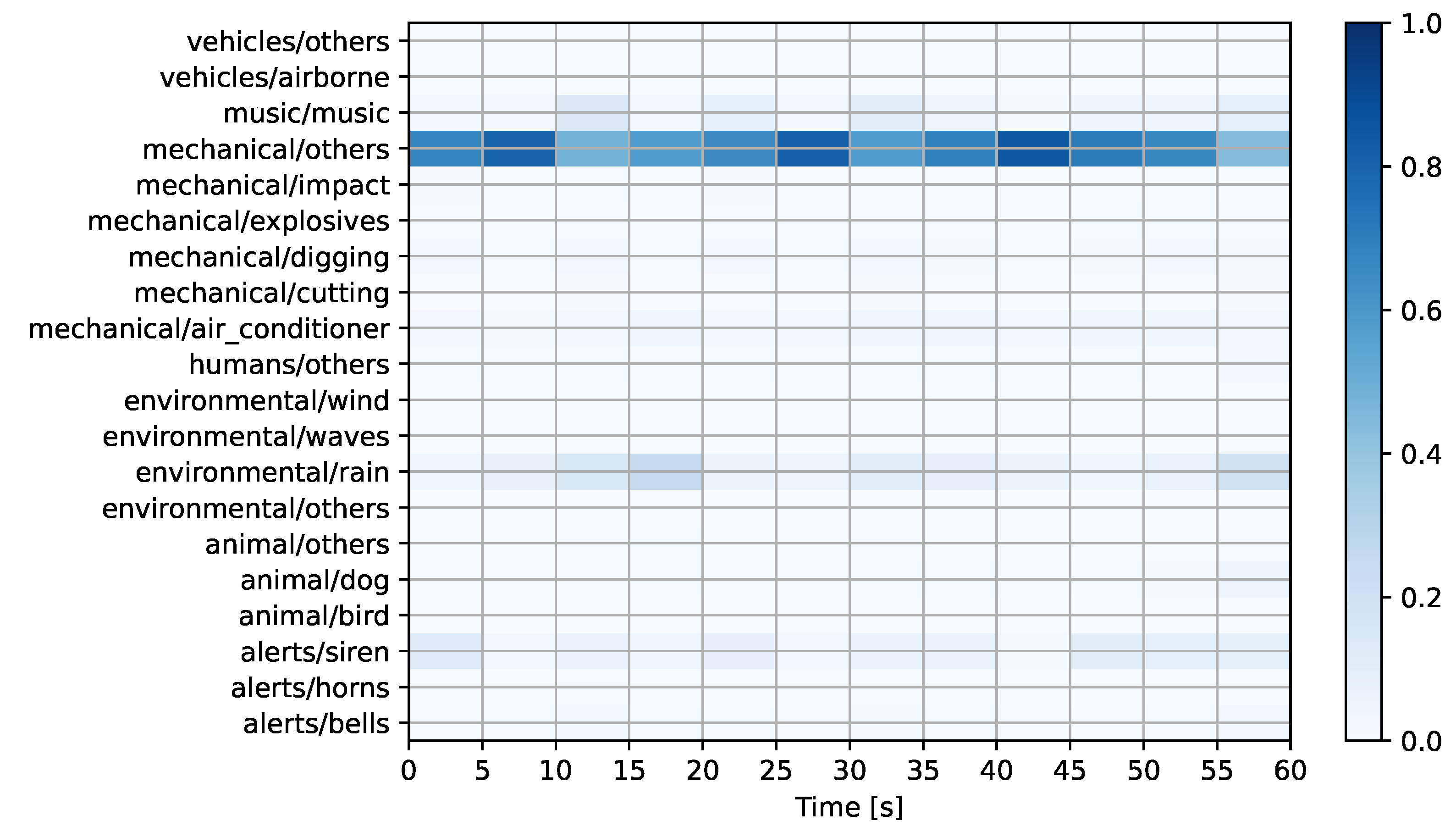For the third audio (see Figure 8), the system once again predicts a mechanical sound in the “others” category. In this case, the prediction was accurate as human experts confirmed that the event corresponded to an engine running within a construction site.

The last stage of the pipeline involved experts auditing the model’s predictions by inspecting the outcome of the persistence filter (three audios). In this case, and for completeness, the entire 115-min subset was inspected by a team of trained specialists that labeled audio events following the taxonomy presented in Table 2. In total, the experts found that three audios of this subset contained the strong and persistent presence of regulation-offending sound events. The performance of the model was then compared to the expert labels (ground-truth), and the results are shown in

Table 7. Classification performance of the model as a function of the detection threshold. Ground-truth is based on human-expert criteria. TP: true positive; FP: false positive; FN: false negative; and TN: true negative.

Threshold	TP	FP	FN	TN
0.3	3	8	0	104
0.4	3	3	0	109
0.5	2	1	1	111
0.6	1	0	2	112

, where:

• True positive (TP): A regulation-offending audio correctly detected by the model.
• False negative (FN): A regulation-offending audio missed by the model.
• False positive (FP): An audio that was incorrectly predicted as regulation-offending.
• True negative (TN): An audio that was correctly predicted as non-regulation-offending.

From Table 7, we can see that for a threshold of $T=0.5$, the model misses one regulation-offending audio while presenting a single false alarm. By decreasing the detection threshold to $T=0.4$, all of the true regulation-offending audios are recovered, but the number of false positives (FPs) increases to three. These FPs (e.g., audio 1654224726 in Table 6) were predicted by the model as mechanical noise, but according to the experts, their content is dominated by environmental sounds of rain and wind with no discernible traces of mechanical sounds. This fact suggests that the robustness of the model predictions could be improved by collecting, labeling, and training with more audio recordings affected by these weather conditions.

Setting a lower detection threshold enables the correct detection of all of the audios in the dataset that infringe upon the regulations, but at the expense of producing more false alarms. The latter directly impacts the labor of the expert in charge of auditing the model’s prediction. However, we note that, even when accounting for the false positives, the number of audios to be reviewed is significantly lower than the entire 115-min subset. In summary, selecting an appropriate detection threshold depends on the available auditing expert capacity as well as the acceptable detection rates that may be expected or required by authorities.

4. Discussion

We noted that only three audios were selected for human inspection by using the machine-assisted pipeline. Compared to the 115 audio files filtered merely by SPL, this quantity indicates a 97% reduction. As a reference, taking the SINGA:PURA urban sound dataset [34], which recorded 1092 min of urban sounds, the application of the FuSA system would return a set of audio files of approximately 29 min, to be analyzed by a trained specialist. As a result, the expert only needs to examine 29 audio files individually rather than 1092. The latter is a significant reduction in the number of audio files to be examined for regulatory purposes. Filtering audio only by SPL does not exclude sound events that do not fall into the categories considered in the regulation, for example, environmental or nature sounds (see Table 3). The manual evaluation of the audio recordings is a laborious, time-consuming operation with minimal efficiency since many audios exceeding the SPL threshold do not correspond to a sound event considered by the regulation.

Taking the above example, a coarse estimation of the time required for this task can be made. Supposing that a human expert needs at least one minute to decide on each audio file, using the conventional methodology, it would take at least 18 hours to analyze the entire dataset. However, with the help of machine learning technology, an equivalent result can be obtained in only about half an hour. Note that the time required to infer the classes for one minute of audio using the neural network is on the order of milliseconds using a single GPU co-processor. This inference time can be further reduced by increasing the hardware capacity.

Performing large-scale out-of-norm detection should be developed further in smart cities. If compliance with environmental noise regulations were automated, it would significantly reduce costs and resources, driving sustainability in cities. Under this scenario, to carry out the inspection, it would only be necessary for the noise measurement stations to be connected to the automatic-noise-source-recognition system and to associate the noise levels with the emissions of the regulated sources. The goal is to improve active real-time noise emissions’ compliance significantly and, as a result, regulatory compliance, which would benefit all stakeholders. First, it would benefit noise-emitting sources as they could better plan their environmental management measures. Second, it would benefit all citizens, who would be protected as the regulation would be widely followed. Finally, it would benefit the authorities because they could enforce the regulations efficiently and timely, thanks to the neural network-based system.

A significant challenge for applying the proposed methodology in other situations is assuring that FuSA’s deep learning model can generalize effectively. As with machine learning applications in general, the generalization capability of a model is limited by how well the training dataset represents the scenario in which the model will be operating. In the case presented here, the FuSA model was trained using data collected from the city of Valdivia using specific recording hardware and settings. If the class distribution changes drastically (e.g., applying the trained model in a city of different characteristics), we would expect a decrease in the model’s performance. This problem may be addressed using transfer learning methodologies, i.e., using a relatively small number of labeled examples from the new scenario (target) to continue fine-tuning the model from the original scenario (source) [26,30].

Future work might use specific technological and methodological developments. The data’s traceability is one crucial example (measurements). Progress must be made in data traceability to ensure there are no risks of data tampering. This issue arises because a certifying officer is responsible for determining whether or not the audited noise source complies with the regulations. Therefore, it would be necessary to devise a system to ensure or attest that the audio recordings and measurements (noise levels) correspond to the audited noise source.

Data privacy is another issue to be addressed. A privacy protection mechanism should be established, especially with speech-related sounds (conversations). The same artificial neural network system should establish a different treatment for audio recordings with human voices or other sounds that may compromise people’s privacy. However, this conflict exists today, as the expert must listen to each of the analyzed recordings.

5. Conclusions and Future Work

Noise sources in urban areas are regulated to operate only at a certain level of intensity and for a limited amount of time. In the regulation process, various stakeholders work together to keep noise pollution at acceptable levels. Collecting information as audio recordings to enforce the regulation is essential. Several monitoring stations are installed at specific city points for this purpose. However, a significantly associated challenge is the large volume of data that must be examined by trained specialists (listening to the audio files one by one). This fact leads to a very high demand for various resources to carry out the work of noise regulation. In this sense, the machine learning tools developed in the FuSA project for environmental noise analysis are presented, applying the current Chilean regulation on environmental noise. The system proved helpful for this purpose, and the number of audio files that required expert analysis was reduced by 97% by using machine learning.

Audio recordings containing significant wind and rain sound affected the system’s performance. Thus, the robustness of the model predictions could be improved by collecting, labeling, and training it with more audio recordings affected by environmental conditions.

The model’s performance relies upon the detection threshold defined in the persistence filter. The correct detection of all of the regulation-infringing audios in the dataset was achieved by setting a lower detection threshold. However, a threshold reduction produces more false alarms. Thus, selecting an appropriate detection threshold depends on the available expert auditing capacity and the acceptable detection rates that may be expected or required by authorities.

The use of additional monitoring stations distributed throughout the city is intended as further work. As part of action plans to reduce noise pollution, the FuSA system is also expected to help keep track of strictly regulated environmental noise sources at sensitive receivers.

Finally, it is anticipated that machine learning methods will continue to be encouraged. Their implementation in the pertinent public services and environmental noise inspections could optimize the procedures for securing the urban environment from the effects of noise; protecting public health; and reducing noise pollution.