Management of Railway Power System Peaks with Demand-Side Resources: An Application to Periodic Timetables

Abstract

The objective of this paper involves the analysis of opportunities for the management of Railway Systems’ demand using Physical-Based models and aggregation tools well-known in “conventional” Power Systems to develop and enlarge the portfolio of Distributed Energy Resources. This proposed framework would also enable the use of railway flexible resources to their use in Power Systems. The work considers trends for the development of railway transportation units through the adoption of technologies that increase the flexibility of railway units. For instance, we mean a set of resources such as onboard generation in dual units, energy storage and generation in last-mile units, and auxiliary loads. Their inherent flexibility can contribute to increasing the management possibilities of the overall net demand. The proposed scenario under study faces some of the energy concerns of periodic timetables: fast and high-power peaks in demand unknown in conventional Power Systems. The simulation results present the achieved flexibility and its potential: a decrease in peak demand by around 20% and an increase in energy recovery by 10%, lagging new investments in infrastructure. These results improve the social and economic benefits of railway transportation on the overall energy and environmental objectives while reducing energy concerns due to the increasing use of railways and boosting the sustainability of the transportation system in the coming decades.

1. Introduction

Sustainable and cost-efficient transportation benefit society, economy and environment. For this reason, different governments worldwide have promoted the development of railway traffic, but this growth has strained infrastructure capacity, especially in Railway Power Systems (RPS). The current RPS capacity must be used as efficiently as possible, minimizing energy cost, and this involves the introduction of new approaches. Consequently, the main concern of this paper is the analysis and evaluation of different possibilities offered by the present technology for the management of tractive generation (e.g., regenerative braking and diesel-electric dual units), non-tractive loads (“auxiliary” loads), static loads (track points) and onboard Energy Storage Systems (ESS) used in railways (e.g., the so called “last-mile” ability of some new locomotives and multiple units). The approach suits the portfolio that different agents of Public Power Systems (PPS) are considering: Distributed Generation (DG), Demand Response (DR) and Energy Storage Systems (ESS), and especially Smart-Grids developments in recent decades. The idea is that some trains (locomotive or multiple units) can be a smart load or generator (a railway “prosumer”) for both the railway and the conventional power systems. In this way, trains can generate energy through regenerative braking (older and new units), on board storage and generation (modern and hybrid units), but also, passenger trains have flexible loads (heating and cooling loads) that can represent up to 10–20% of demand [1]. Moreover, the efficiency and greenhouse emissions in transportation are important concerns for public authorities [1], and this work also depicts some developments in this area.

The interest of regulators and public authorities to improve the service to their citizens has evolved to the development of the so-called “periodic timetables”. The idea is that train patterns repeat after each scheduled period, for example, at the same minute every hour or every half hour (e.g., 8 h 11 min, 8 h 41 min, 9 h 11 min, 9 h 41 min…). This type of schedule is very easy to remember for the customer, and it also enables the management of its railway journey in a specific route. Periodic timetables have been used in several countries in Europe (e.g., Netherlands or Germany) for many years and are being introduced in other European railway systems. A reference in the literature is Switzerland. The Swiss railway timetable is an effort that began in 1982 (the Bahn/Rail 2000 initiative [2]) and, according to some experts, it has been one of the main factors behind the efficiency and growth of railway transportation in this country. The overall foreseen growth in rail demand (passenger per km) ranges from 20 to 80% (in some cases) between 2012 and 2030. Switzerland already has train services every half hour that connect the major population areas, but operators are evolving to the idea of raising this frequency to 15-min by 2030–2050 [3]. In practice, this entails that those tractive loads switch-on at the same time and require a high-power demand to accelerate the train in a short time (some minutes). Some researchers expect an average increment of demand by 25%; and even 40% at peak times in the next decades [4]. Moreover, to accomplish timetables, locomotives and units are increasing their rated power to gain acceleration performance in train steps, raising demand requirements. For instance, this synchronization of departures is a primary factor that explains oscillations up to 300 MW (in 5 min) in the demand curve of the main Swiss railway operator (SBB-CFF-FSS), according to different reports [3]. These problems are well known in power systems but with lower rates for demand increase and lower frequency of changes (for instance, in the integration process of PV resources). That is, some typical problems in PPS are even bigger in RPS, especially when railways manage their own power system (the case of Switzerland, Germany or Austria at 16.7 Hz for traction supply). Because of these issues, the Swiss operator SBB started in 2018 a study to evaluate the possibilities of DR in “power loads” [4]: Heat Ventilation and Air Conditioning (HVAC) loads in coaches and heaters in point tracks (around 13,000 points in the Swiss system).

The railway timetable acts as the basis for planning processes within the railway system: the rolling stock performance, circulation and maintenance, the staff schedules, the infrastructure and, from the point of view of authors, the management of energy costs and its portfolio, as seen in Figure 1. Future and actual costs from the point of view of Railway power system operation are basic issues for its sustainability and efficiency [5].

Consequently, the use of DG, DR and ESS (i.e., Distributed Energy Resources, DER) portfolios must be considered as a relevant tool in the future framework of the new electricity supply paradigm: Smart-Grids. According to this paradigm, the interaction of the Electric/Public Power System (PPS) and the Railway Power System (RPS) should bring new opportunities to perform a better and more reliable operation of the overall energy system. The main contributions of this paper are two. First, the paper integrates different models for main loads of trains (traction), secondary or auxiliary loads (or “hotel/comfort” loads), and main onboard ESS (OESS) to evaluate the flexibility of train’s demand and their aggregation to calculate the overall demand. Secondly, the paper demonstrates the potential of DER resources to reduce load peaks and energy requirements and to improve the operation of the RPS, as well as the discussion of the use of those resources for balancing. The rest of the paper is organised as follows: Section 2 describes the scenario and methods used, explaining the models applied to simulate tractive, auxiliary loads and OESS systems. Based on these models, Section 3 depicts the present possibilities for using ESS and DR to reduce power peaks due to synchronization policies. Section 4 presents some simulation results for the alternatives described in Section 3. Finally, some conclusions are summarized in Section 5.

2. Materials and Methods

2.1. Methodology Overview

This section presents the scenario used for simulation and a review of the different methodologies that have been used in this paper. All these methods are based in the search for physical knowledge in processes that drive the dynamic behaviour of the different elements of the system (HVAC loads, tractive units and storage through ultracapacitors or batteries). The reason for this choice is that this approach easily allows the interaction with other tools developed for DER in the literature, some of them developed by authors in previous papers [6].

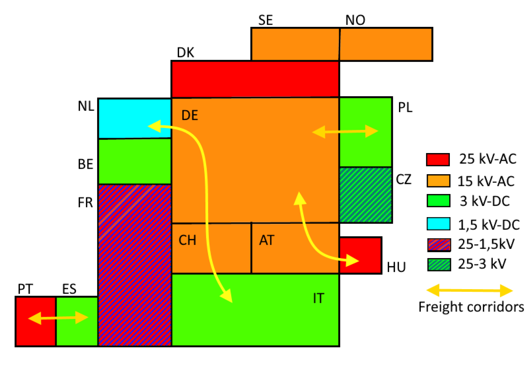
2.2. Sustainability Scenario: The Transportation Sector in the Horizon 2030–2050

The transport segment is one of the main emitting sectors worldwide. For example, it is the second in the European Union [7], representing around 25% of the total greenhouse emissions (the second sector in this “dark” ranking after the energy supply segment). For this reason, it is a key sector related to achieving environmental targets in most countries, especially developed countries. In this segment, railways appear as the most sustainable mode of transportation. Some data are relevant to support this assertion: the rail subsegment accounts for 1.8% of the total EU energy consumption in the overall transportation segment, while in 2016 [7], it contributed 6.6% of passengers’ transportation and 11.2% of freight. Unfortunately, the COVID-19 pandemic has decelerated this trend (public transportation versus individual cars), and obviously, there is still considerable room to increase these shares if public authorities engage the support of railways.

Railways have another advantage with respect to sustainability: the lifetime of vehicles (coaches, locomotives, and EMUs) and modularity. While the average life of its competitors (car, bus, or trucks) is around 10–15 years and around 300,000 km, the life expectancy of a rail vehicle can reach 30, 40 or up to 50 years (some freight or passenger units) and around 5,000,000 km. For these reasons, railway vehicles are well suited to incorporate new developments and systems during their lifetime that increase their efficiency and decrease emissions.

In research programmes, railways have gained momentum. For instance, in the new research programme EU-Rail of the European Union [8]. It is interesting to remark on “Flagship Area 4” of this programme that deals with sustainable and green rail systems. According to this research line, key topics are focused on “Developments oriented towards a more integrated and standardized Rail Power Smart Grid, integrating greener energies, cutting peak of energy consumption and allowing for a better control and management” and “Developments oriented towards a better energy management at station level”. Both aspects (peak of demand and the management of energy at stations) are considered in this paper through “enabling technologies”: energy storage systems, onboard generation, and load management.

It is important to consider that railways are directly and indirectly responsible for three types of emissions [9]: direct emissions from their trains, the purchase of energy from conventional sources for buildings, stations, the production of vehicles, and the development of new infrastructure. The electrification of railways increases their efficiency and reduces some of these emissions (according to the generation “mix” in each power system), but also diesel units (i.e., high-emission vehicles) can benefit from those “enabling technologies”. For example, the use of energy storage enables the decoupling of the demand of diesel–engine, allowing a duty cycle at points of maximum efficiency and the recovery of braking energy. Finally, “comfort functions” in the passenger service (i.e., so-called hotel loads) are of interest. Direct and indirect savings can be found through more efficient thermodynamic cycles (CO₂) developed for other energy segments [10], the control of ventilation according to occupation (about 20 m³ of fresh air per seat and hour can be considered for passenger service, and this flow represents heat losses) or changes in the heating patterns of passenger trains in yards during night periods in winter (this can explain around 10% of the overall demand of these vehicles in some countries). These considerations about sustainability concerns define the framework and the interest of this research.

2.3. Energy Scenario: Energy Share in Passenger Rail Units

Main energy end-uses in railways can be classified into tractive and auxiliary/hotel power loads. Auxiliary loads can be classified into variable and constant loads. Figure 2 depicts an approximation of end-uses share. Notice that this share depends on the kind of railway being considered (e.g., metro, suburban, intercity, high speed…) and the type of units (full electric, diesel-electric, diesel-hydraulic, hybrid…) and service (passenger or freight). In any case, many of these uses exhibit some level of demand flexibility. For instance, tractive energy can be modulated through the reduction in the speed or acceleration, because some dwelling time is considered in the planning of services to face contingencies (i.e., service delays or congestion of tracks). Moreover, setpoints of air conditioning or heating can be also changed to some extent without causing a severe impact on customers. Summarizing, some interesting flexibility can be found in railways.

2.4. The Simulation Scenario: A periodic Timetable for a Terminus Railway Station

Terminus stations are very usual in England (King’s Cross), France (Paris Montparnasse; Paris Gare du Nord), Switzerland (Zurich Hbf, Luzern), Germany (Munich), Italy (Milano) and Spain (Alicante, Madrid Atocha and Madrid Chamartín). In these stations, intercity and regional trains are parked on the platforms or have arrived up to 10–20 min before they leave the station to allow check-in for travellers or because of transfer requirements with other trains. Moreover, periodic timetables entail that these dwelling times should be known in advance with a high degree of accuracy. In these cases, trains on platforms require power for auxiliary loads and can store energy (from regenerative braking of other units that arrive at the station) or are able to generate some power from OESS. Moreover, dual units (with diesel and electric engines) can generate power similar to conventional DG units, for instance, in the case of diesel-electric shunting locomotives used in terminus stations for the triage of coaches or, alternatively, through some standard diesel-electric locomotives modified and endowed with a pantograph, as proposed in [11].

A timetable for a medium-size passenger station, Luzern (CH), is shown in

Table 1. Timetable for S-Bahn/Suburban (S), RegioExpress (RE), InterRegio (IR), Eurocity/Intercity (EC/IC) services in the afternoon (hour 1X, specifically from 14 h to 15 h), 2022, Luzern, CH.

Arrivals					Departures
Service	Time (min)	Origin	Op	Platform	Service	Time (min)	Destination	Op	Platform
IR 15	01	Bern/Geneve	SBB	4	IR 15	00	Bern/Geneve	SBB	8
S4	02	Stans	ZB	14	S9	02	Lenzburg	SBB	10
RE+RE	03	Langenthal&Bern(2)	BLS	5	RE	05	Olten	SBB	9
IC 21(1)	05	Basel	SBB	7	RE	06	Interlaken	ZB	13
S1	07	Baar	SBB	3	S3	06	Brunnen	SBB	11
S1	15	Sursee	SBB	10	IR 70	09	Zurich	SBB	6
S5	17	Giswill	ZB	14	IR	10	Engelberg	ZB	12
IR	21	St Gallen	SÖB	2	S5	12	Giswill	ZB	12
IR 75	25	Zurich/ Konstanz	SBB	5	S1	14	Sursee	SBB	3
IR 27	30	Basel	SBB	15	S6	16	Lagenthal and Langnau	BLS	5
S4	32	Wolfenschiessen	ZB	14	IC 21 (1)	18	Lugano	SBB	7
IR 26	41	Locarno	SÖB	7	S1	21	Baar	SBB	10
S6	43	Lagenthal&Langnau	BLS	5	S4	27	Wolfenschiessen	ZB	14
IR	49	Engelberg	ZB	12	IR 27	28	Basel	SBB	4
IR 70	51	Zurich	SBB	6	IR 75	35	Zurich/ Konstanz	SBB	5
S3	53	Brunnen	SBB	11	IR	39	St Gallen	SÖB	2
RE	55	Interlaken	SBB	9	IR 26	54	Basel	SÖB	7
IR	55	Olten	ZB	13	RE+RE	57	Langenthal and Bern (2)	BLS	5

⁽¹⁾: Not scheduled every hour; ⁽²⁾ Service coupling/split in Wolhusen.

, with traffic around 100,000 pas/weekday. Table 1 depicts arrivals and departures. Logically, trains apply regenerative braking to the overhead line of RPS (15 kV 16.7 Hz, in this case) whereas some other trains leave or are ready to leave in the very-short term, demanding load for auxiliary services, for example, the heating of coaches, or to accelerate. The main characteristic of this timetable is that it is basically the same for every hour from 6 a.m. to 11 p.m., although Luzern is not a “full” node of the Swiss periodic timetable. Four railway operators provide passenger services: BLS AG [12]; Südostbahn (SÖB, [13]); Zentralbahn (ZB, [14]); and SBB-CFF-FFS [15]. SBB is the main operator, and it can be considered as a potential railway “demand aggregator” to manage the electricity consumption of its trains (demand, capacity, efficiency and flexibility) both in RPS and PPS.

The literature states that the use of periodic timetables has several advantages for the user (simplicity), but some problems for the management and operation of trains arise. For instance, the stress of infrastructure resources in the case of time delays [16], or the use of rolling stock near its operational limit to fulfil time requirements. Several papers deal with the design of timetables and discuss several optimization methods for the resolution of the problem, considering some constraints such as the transfer of passengers in stations [17], the planning of rolling stock circulation and the maintenance of the infrastructure, both from the point of view of train operating companies and infrastructure managing companies [18]. Most of these approaches define the infrastructure, crew journeys, line junctions and crossing points, but do not consider the energy problem in detail [19] during the planning process. On the other side, some works in the literature consider the problems that are generated by timetables, for example to elaborate solutions for evaluating the overloads and under-voltages that timetables produces and to achieve robustness against them [20]. Finally, the so-called train cooperation (the use of braking energy for the acceleration of trains) is discussed in [21] to obtain an optimization of train dwelling times in stations, but acceleration and braking models are too simple, and storage and other DER are not considered. The present work intends to introduce timetables from an energy perspective, considering DER portfolios.

Table 1 also includes the track or platform for the arrivals and departures. This information is of interest because the reader/researcher can foresee if the same physical unit arrives and performs later the same or another service (i.e., if the train is parked in the station, it demands energy for ancillary loads and is available as DER). Timetable planners use a clock for each node (basically a railway station) that represents the arrivals and departures, in minutes, for a specific service (S, RE, IR, IC…). The axis of symmetry of these journeys defines the kind of node (00, 15, 30, 45…). In this case, (Figure 3), some services in Luzern present 00 or 30 symmetries (IR70 and 75, RE), but not in all cases (S1 and especially IC). For this reason, in practice, Luzern is not considered as a conventional nodal point (or an “integrated fixed-interval timetable hub” [5]) for the Swiss periodic timetable system. Forecasts show a horizon of services every 15 min in all the system [22] by 2050 that will probably increase average, oscillations and peaks in demand. This constraint must be carefully considered for timetable planning as it is proposed in Figure 1.

An additional reason to choose Luzern as the simulation scenario is that Swiss railways (in this case, SBB-CFF-FFS) own a small power system (RPS, 600 MW) which includes six hydroelectric power plants at 16.67 Hz (a usual frequency for traction in Central and Northern Europe) which deliver power to railway substations at 15 kV-AC (at 25 kV in some systems). The problem is that this system is not an islanded one because of the growth of passenger and freight traffic in Switzerland. The increased demand in recent decades has involved additional requirements for energy supply by Swiss PPS through seven AC/AC converters (50 Hz to 16.67 Hz) [4]. Average demand reported in the technical literature by SBB operators is presented in Figure 4a. According to the data discussed in [4] demand exceeds 16.67 Hz generation capacity of RPS (around 450 MW) in the morning and the afternoon. These peaks are covered by frequency converters (Figure 4a, dashed lines) and this energy is bought in energy markets.

Another characteristic is that the peaks in RPS are quite different from the peaks in PPS. Usually, in RPS, peaks occur for a noticeably short period, typically less than 1–2 min (30, 45, or 60 s) due to acceleration and the tractive characteristics of trains. Those peaks are not shown in Figure 4a because the demand curve in Figure 4a is an hourly curve that “filters” demand changes, but these peaks are important and will be analysed in Section 4 through simulations. Usually, demand peaks appear during peak traffic periods (7–8 a.m. and 6–9 p.m.) and involve changes up and down around 15–25 MW/s (on the RPS), which requires the use of additional power converters to cover these peaks (they are usually more frequent in winter). Demand swings can reach up to 300 MW (RPS) in a 15 min period [4]. Notice that this scenario is worse than power engineers must face in PPS, where infrastructures operate with slower fluctuations of demand. Those fluctuations in power systems explain the interest in DR policies worldwide and make possible the deferral of new and expensive investments. With some adaptations due to the particularities of railway loads, a similar portfolio should be of interest to RPS too.

It should be noted that RPS peaks involve serious penalties for railway operators. In the example of Swiss railways, several issues must be considered. First, the capital cost of converters to cover peak periods (Figure 4a, area from 500 to 750 MW). Second, the cost of energy in markets during periods where SBB hydro generators do not cover demand and short-term periods causing unbalance in RPS. Figure 4b depicts an example of energy prices in winter and summer periods according to EPEX day-ahead market data [23]. Demand peaks follow peak prices. Moreover, intraday markets can reach high prices in those periods [23], i.e., energy costs increase by 30–40% due to these peaks of demand. These conditions represent a typical scenario for applying DR policies that has been explored by SBB since 2018 [4], but firstly focussed on coach heating loads and point heating systems in the track.

2.5. General Equations of the Motion

For simulation purposes, this work applies a physical-based model for the acceleration, a, of a train or locomotive. This is a scalar equation and depends on the equilibrium between external and internal forces on the train/locomotive:

$$(m+J/R^2)a={\displaystyle \sum _{k=1}^n{F}_k}$$

(1)

$$m\left(1+k\right)a={\displaystyle \sum }_{k=1}^u{F}_{tk}-{\displaystyle \sum }_{k=1}^u{F}_{rk}-F_c-F_g-F_s-F_b$$

(2)

where:

n: overall number of effects being considered.

n: number of elements of the train: locomotives, rake, multiple unit…

m: mass of the train

a: acceleration of the train

k: equivalent rotational mass due to inertia

J: moment of inertia of the different rotating masses (wheels, motor rotors…) in the transmission which causes an apparent increase in mass.

R: wheel radius.

F_k: propulsive/resistant forces

F_tk: propulsive force, tractive effort of locomotive/EMU k of u units in the train.

F_rk: resistance forces due to the element r of the train, locomotive, coach, generator…

F_c: curve resistance

F_g: grade resistance due to the slope of the track (positive or negative)

F_s: starting resistance

F_b: braking resistance due, for example, to dynamic braking (curves can be found in [24], obviously for motor units) and air braking (a detailed model is analyzed in [25])

In this model, k is the increment of mass due to rotating inertia that ranges from 0 to 0.30, depending on the type of vehicle, usually in the range [0.06, 0.10] for a complete train, according to [24]. For specific units, a more accurate value must be used from specific sources (manufacturers, tests and literature) to reduce the error. For example, in [26], k = 0.08 is reported for commuter motor units and 0.06 for trailer units. Some additional discussion and values can be found in [25]. In [27], for conventional trains in some intercity services (locomotive and coaches), k = 0.22 and k = 0.06 have been used in Equation (2).

Resistance forces are the sum of all forces acting on the train at a given time or place. These resistance forces can be examined in detail with different models [24,28] but they are not the main objective of this paper. A quadratic formula has been used to approximate rail vehicles resistance:

$$F_r=A+Bv+{Cv}^2$$

(3)

where v is the speed of the vehicle (m/s), and A (N), B (N s/m) and C (Ns²/m²) are regression coefficients obtained by fitting run-down tests of passenger and freight units to the previous equation.

This paper uses different data from manufacturers (Bombardier, Alstom, Patentes Talgo, Stadler Rail, Siemens, EMD…), associations (UIC) and railway administrations (SNCF, DB, SBB-CFF-FFS, ÖBB…) both for cars (e.g., Eurofima, Talgo VI-VII or Corail), locomotives (e.g., “BoBo” such as SBB-Re460, RENFE S-253 or “CoCo” such as RENFE-250) and compositions of homogeneous and composite materials (SNCF, RENFE). The portfolio of units manufactured in different countries, and used by railway operators, can be considered similar or the same in some cases (e.g., high speed EMU in Spain and France, or VECTRON and TRAXX locomotives in service by many EU railway operators). This fact makes easier and more representative the presented results instead of the fact that simulated units are not exactly the units in service. Notice that the composition of trains can change for different services and days because of a different passenger demand or the availability of rolling stock.

With respect to grade resistance:

$$F_g=mgi$$

(4)

If the slope is β, i = sinβ, the curve resistance is found by means of empirical formulae. Some expressions in the literature are different for different curve radii, but this does not make much sense. New and interesting approximations and equations for this force can be found in [29], for instance, according to [29]:

$$F_c=0.001 mg\ast 198/r_c$$

(5)

where r_c is the curve radius.

With respect to starting force F_s, there have been very limited studies on this topic. An accurate approximation of the main interest for haulage is the approach proposed in reference [30], especially for freight trains. In this model, when the vehicle has zero speed, the value of starting resistance is assumed to be three times the value for v = 10 km/h in equation (3); when the speed is between v = 1 and v = 10 km/h equals the value of (3) in v = 10 km/h. Finally, it linearly decreases between the values v = 0 and v = 1 km/h.

2.6. Traction Effort Curves and Other Considerations for Simulation

Propulsive forces (F_tk, Equation (1)) are basic both for the accurate simulation of trains and to calculate demand peaks due to timetables scheduling. Electric locomotives and vehicles (e.g., electric multiple units, EMU) have greater performances when they are compared with diesel-electric locomotives and vehicles (DMU). It can be observed that the performance in steady state is higher (up to 100%) for electric locomotives than in diesel locomotives. In the simulations to be presented in Section 4, electric locomotives can develop up to 5.6 MW (according to their tractive effort characteristics, Figure 5a, red curve and orange in dash-dotted line) whereas a diesel-electric locomotive is limited to around 2.4–3.6 MW by the power of its diesel motor (in the case being considered, the Spanish series S334, rated power of engine 3300 HP). In addition, an electric locomotive can be asked for a higher power during a short time and the acceleration is higher than in trains with diesel-electric traction. The possibility of regenerative braking is another advantage, and, consequently recovers some energy costs. Some manufacturers argue that diesel traction doubles energy costs for the same train load (a specific comparison is made between a “Maxima CC40” diesel locomotive by Voith [31] and a 5.6 MW TRAXX series in [32]). These evaluations and environmental constraints will produce a premature and unjustified withdrawal of diesel units before the end of their lifetime. A “second life” for some upgraded units is envisaged in Section 4.

However, diesel units have advantages in lines with low traffic, and in duties that involve the change between different voltage sections in national or international corridors (Figure 6, for some European systems) or to haul trains in industrial terminals without an additional freight locomotive (in “last-mile”, LM, option). This has been a main reason for the punctual success of some diesel locomotives (e.g., Euro 4000) for freight duties during the deregulation of railways in the European Union. Moreover, in the case of a failure in the catenary or other RPS infrastructure, diesel-electric units are a valuable resource to avoid congestions in tracks.

However, hybrid units, DHMEU, in the diesel mode of operation, have several advantages to be discussed later in this work, for example, a high traction effort (Figure 5b). Specific characteristics for diesel and electric units with high storage requirements (i.e., around some MWh) for heavy haul operation, B unit ESS powered locomotives (without a cab, used in Australian and US railways) can be found in [33].

At the same time, there are also significant differences in the braking performance of the different locomotives. The maximum braking power for the two full-electrical locomotives is about 5.6 MW, however, the maximum braking effort is higher in BoBo S-253 (240 kN, manufactured in the year 2007) than S-252 (168 kN, year 1992). In the case of the hybrid locomotive/vehicle, the maximum braking power is 4 MW. Finally, diesel-electric locomotive S-334 (a refurbished series in the year 2006) only can achieve a braking power around 1.9 MW. For this reason, diesel and hybrid locomotives require more time to reduce velocity or completely stop a train if only regenerative braking is applied.

With respect to trains (locomotives and EMUs), this work considers trains with the characteristics described in [27]. Two reasons justify that choice. The first is that main railway manufacturers (Bombardier, Alstom, Patentes Talgo or Siemens) supply similar locomotive and motor unit families for different EU countries (e.g., TRAXX or VECTRON locomotive series, or Flirt EMUs by Stadler Rail). The locomotives that have been simulated are considered of TRAXX series [23] (around 6 MW of rated power, 15 kV/16.67 Hz) with coaches for IC services, small power EMU for suburban services (0.75 to 1 MW of rated power) and larger EMU (from 1.5 to 4 MW of rated power) are considered for IR and RE services. The second reason is that this work intends to discuss issues and alternative solutions for energy swing patterns due to timetables, but not to achieve accurate consumptions on a specific system, operator, track or substation.

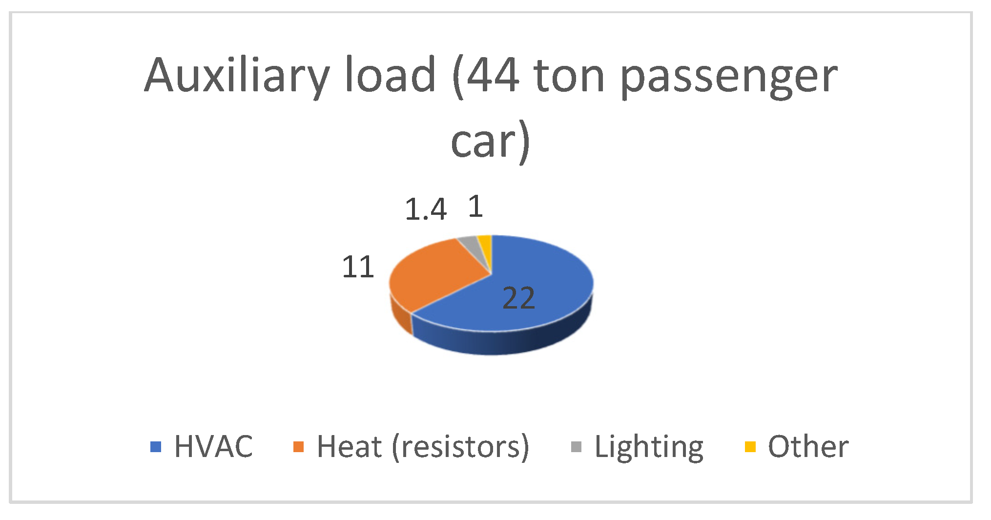
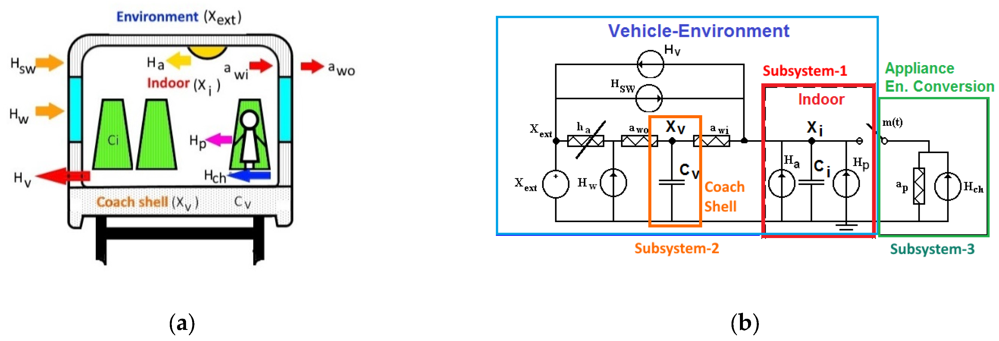
2.7. Ancillary Loads Model: Hotel Loads in Railways

In railways, the electrical load in passenger units (coaches in conventional trains) are due to lights, ventilation, heating and air conditioning, information screens, opening and closing of doors or grills and cooking in bistro and restaurant cars. These ancillary loads are also referred to the technical literature as “hotel loads”. UIC estimates that the amount of energy needed for hotel loads ranges from 10–15% up to nearly 40–50% (in some cases) of the overall demand of the train [1], see also Figure 2. In [24], authors estimated main auxiliary loads for standard coaches of the Spanish operator (RENFE) in 1980 and 90 (series 9000 and 10,000), see Figure 7. These series are very close to the 42 T European Standard Coaches class called “Eurofima” (European Company for the Financing of Railroad Rolling Stock) delivered in the late 1970 s and refurbished in the 2000 s. Some of these coaches, due to their performance, are still in service in many countries, being used for IR and IC services.

Auxiliary loads can be directly supplied by the locomotive, but this option involves a reduction in traction effort or, alternatively, they can be supplied from the catenary through converters in coaches (AC/DC or DC/DC converters). This option makes easier load management of such loads. In some cases, trains are fed from technical cars placed at the ends of the rake. Each power car is installed with one or several DG sets generating 3–phase (4 wire) power supply at 3 kV DC or 380 Volts 50 Hz. Obviously, in a train with 8–10 cars, this load can be of interest and is a kind of load well known in the demand response portfolio on other customer segments, such as residential and commercial demand [6]. For this reason, their flexibility potential should be analyzed in RPS. Main differences between railway hotel/comfort loads and residential loads are the capacity for heat storage (i.e., the specific heat of materials, bricks and concrete in buildings vs. aluminium and steel in railway vehicles). Moreover, railway coaches require the supply of fresh air to maintain indoor CO₂ levels, and, finally, the effect of speed in the exchange of heat between the vehicle and its environment due to convection effects, which can change significantly heat loss coefficients. In our application (railway timetables), the last factor is not considered because arrivals and departures are undertaken at “low” speeds, and most of the management time units are parked in the station.

The methodology used in this paper is also based on physical-based models (PBLM), the same option used for tractive loads. The main idea is that heat exchanges in train coaches are similar to heat exchange in buildings but with different response characteristics due to the use of different material for envelopes and different surface (%) for windows. Moreover, energy conversion devices (electricity to heat) are similar: compressors, condensers and evaporators, even in their size. The models for HVAC load in trains are based on previous developments of authors in residential segments [34] and the models developed by the laboratory Rail Tec Arsenal Fahrzeugversuchsanlage (Austria) which is an expert in climatic tests for transportation vehicles [27].

Both options use a second order model (type 2R2C) with two or three subsystems (see Figure 8a). Some of the main parameters of the PBLM model can be found for different unspecific trains, coaches or units in [35], and for specific Spanish units in [27]. In the present work, authors have integrated both models for HVAC loads inside the train and have revisited a procedure to aggregate demand for elemental HVAC units inside each coach of the train (from 3–4 cars in suburban services to 8–15 cars in IR and IC). An example of these PBLM models for a Spanish 12 T coach “Talgo VI” (Figure 8b) is depicted in Figure 8c. The state-space system representation is conducted using Equation (6), as follows:

$$\left(\begin{array}{c}\frac{d{X}_i\left(t\right)}{dt}\\ \frac{d{X}_V\left(t\right)}{dt}\end{array}\right)=\left[\begin{array}{cc}\frac{-a_{wi}}{C_i}& \frac{a_{wi}}{C_i}\\ \frac{a_{wi}}{C_V}& \frac{-\left(a_{wi}+a_{w0}\right)}{C_V}\end{array}\right]\left(\begin{array}{c}{X}_i\left(t\right)\\ X_V\left(t\right)\end{array}\right)+\left[\begin{array}{ccc}0& \frac{-1}{C_i}& \frac{-1}{C_i}\\ \frac{a_{w0}}{C_V}& 0& 0\end{array}\right]\left(\begin{array}{c}{X}_{ext}\left(t\right)\\ H_{ch}\left(t\right)\\ H_V\left(t\right)+H_{SW}\left(t\right)\end{array}\right)$$

(6)

The proposed model includes the consideration of three connected sub-models or sub-systems depicted in Figure 8a,b. The first sub-system explains, from a thermal point of view, all the flows in the interior of the vehicle that interact with the vehicle shell and energy conversion processes to heat from internal appliances/devices (e.g., lighting, passengers, sub-system 3) and the outdoors (e.g., solar radiation through windows). The second sub-system consists of the exchanges of heat through the vehicle shell, between the interior and the outdoor environment. Finally, sub-system 3 considers the conversion of electric energy to thermal energy to provide heating and cooling to the vehicle system. Sometimes, this sub-model is called the electrical sub-model of the load because it defines demand and energy conversion. The structure of this model enables the retention of the other two sub-models when, for instance, coaches improve their HVAC system (sub-model 3 changes), or when coaches are refurbished (envelopes, windows…; and this changes sub-model 2). A common example of the application of circular economy in railways has been applied since the deployment of railways in the XIX century.

Sub-models 1 and 2 use an electric-thermal equivalent, which considers the external area of the vehicle (A), the global thermal transmittance coefficients (a_w0 outdoor-vehicle shell, a_wi indoor-vehicle shell), the heat capacities of the vehicle (C_V and C_i, which define the thermal storage capacities of each coach) and the heat losses and gains through: solar radiation in windows and shells (H_W, H_SW), ventilation (H_V), ancillary appliances (H_a) and passengers (H_p). Finally, the energy conversion (H_ch) from electricity to heat is considered in sub-model 3 (coefficient of performance, voltage level, ancillary electrical heaters…). A more detailed explanation of these parameters can be found in [6] and [10]. Figure 8b shows the overall system model, and Figure 8a depicts the heat flows in the passenger car and the environment.

For simulation purposes, the following parameters have been considered: h_a = 2.49 kW/K; a_wo = 36 kW/K; C_i = 3MJ/K; a_wi = 36kW/K and C_v = 30 MJ/K. A broader range of values, for a comparison between different railway units, is shown in

Table 2. Comparison of heat transfer coefficients for PBLM models and heat capacities of different European vehicles according to [35] (k and K_veh) and a Spanish vehicle used for simulation in [27].

Kind of Railway Vehicle	Sub-System 1			Sub-System 2
	k (W/m2K)	awi (kW/K)	C = Ci (MJ/K)	Kveh (W/K)	aw0 (kW/K)	CV = Cveh (MJ/K)
Metro 1–4 (1)	2.4–3.1	N/A	46–94	48–5479	N/A	5.7–19
Regio 1–4 (1)	1.3–1.7	N/A	13–64	217–1366	N/A	4.6–37
Main (IC) 1–2 (1)	1.4–1.6	N/A	0.72–2.6	93–564	N/A	3.9–24
Talgo VI	N/A		3	N/A		30

⁽¹⁾ Range of values from on-site tests from different units, according to reference [35], Rail Tec Arsenal Fahrzeugversuchsanlage, Wien, Austria

.

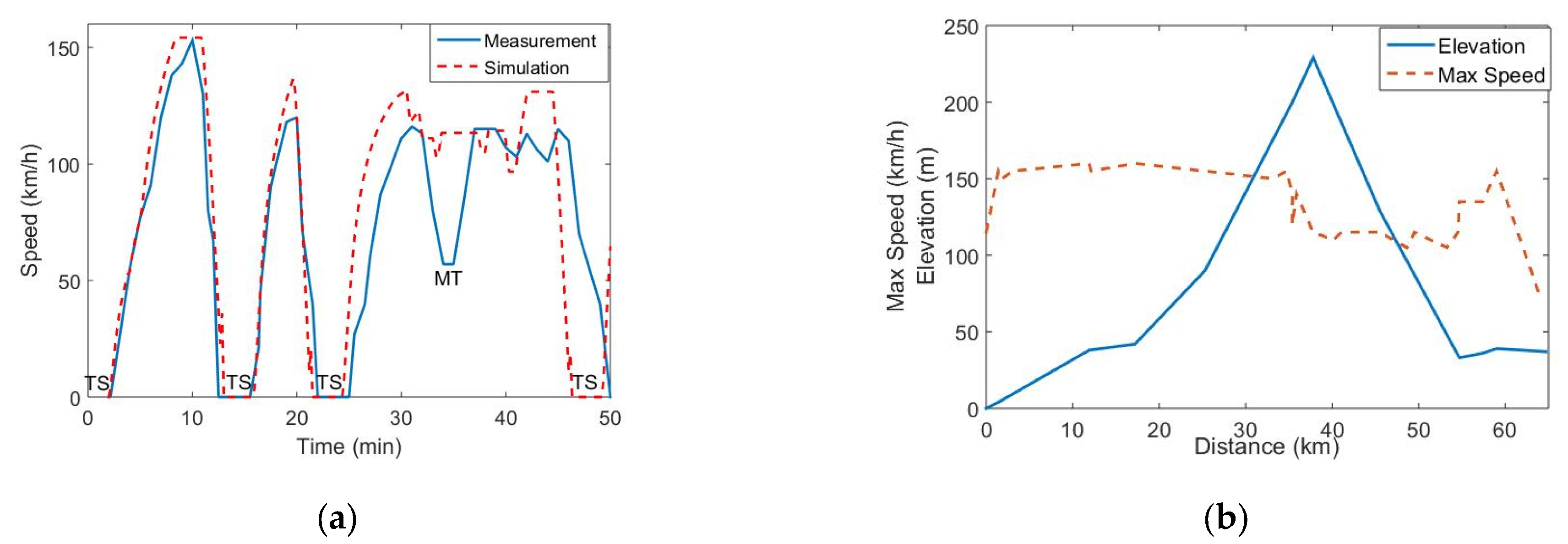
2.8. Validation of the Proposed Railway Models

The accuracy of models has been validated indirectly through the measurement of actual speeds of some classes of the trains used for simulation. In our case, some measurements have been recorded from information panels of those units. Diesel and hybrid units were selected for those tests. For instance, Figure 9a depicts the real and simulated speed of a dual hybrid DHEMU in diesel mode (S730) on 65 km stretch with four stops in Spain. This route has been used for validation due to its characteristic profile (slope) and its maximum speed changes (Figure 9b).

The railway route has four stops on its passenger service. As depicted in Figure 9a, the unit cannot reach its maximum allowable speed in diesel mode (180 km/h) nor the maximum speed of the section (155 km/h) due to the slope between the third stop TS and MT. This can be due to driver behaviour or some temporary speed restrictions in the stretch (the same problem arises in MT, a trenched track with problems in sub-ballast due to periodic heavy rain episodes). This is difficult to know “a priori”. Additionally, the model fails in the acceleration before the fourth TS, and in some braking periods, especially after 45 min. This can be because this TS is a junction station and traffic increases near TS, and also because our braking model prioritizes dynamic braking (for energy targets) whereas the unit also uses an air brake, which acts slowly due to using pressurized air. Considering these scenarios, the Mean Absolute Percentage Error (MAPE) ranges by 8.2%, and it is lower (<4%) for acceleration and deceleration cases (from first TS to third TS,) which is the main concern of this paper: the study of arrivals and departures from/to a station.

With respect to onboard ESS, conventional models for the fast discharge of ESS elements described in the specific literature [36] and discussed in reports from railway research projects were considered [37]. The present simulation uses the models developed in [27] and tested with two banks of Maxwell super/ultracapacitors. Models for residential and building HVAC loads (2R2C) have been described and validated in several papers through demonstrators [6]. The railway car parameters from real tests in [35] have been applied to those models. The tunning of the parameters for each specific case has been conducted through the use of genetic algorithms.

3. Distributed Energy Resources in Railways: Timetables and Demand

3.1. Last-Mile and Dual (Hybrid) Locomotives and EMUs

In the last decade, several railway manufacturers have introduced electric locomotives fitted with a small standard industrial engine (rated power from 200 to 400 kW, a cheap and robust alternative) coupled with an electric generator unit for short-distance operation away from the catenary supply. This option is called “last-mile” [32]. In recent years, battery and ultra/supercapacitor (SC) options, instead of using small diesel generators, are also available in the so called Full-Electric Last-Mile (FELM) units.

The last-mile option is first considered for the DER portfolio because of its flexibility and efficiency. It is ideal for use in freight duties because trains can deliver goods in the “last-mile” without stop transition, i.e., places such as ports, container terminals, good yards or locomotive depots, where some diesel shunting locomotive must be called to help electric locomotives or freight cars reach the end track sections, usually non-electrified. This possibility offers a more rapid transportation service than the competing freight operators reducing emissions on surface transport. Other “new” opportunities for LM units are restricted areas with low noise emission constraints or with zero gas exhaust [38].

Another justification for operators to engage “last-mile” options in their locomotives and units is due to crossing borders between two regions (e.g., Spain, France) or systems that rely on different voltage and frequency RPS. For instance, between Germany (AC, 16.7 Hz) and France (25 kV 50 Hz, and 1.5 kV, DC), or Switzerland (AC) and Italy (3 kV DC), see Figure 6. The last-mile option makes shunting possible in border stations, where voltage and frequency change. e. In addition, from the point of view of contingencies in the RPS (e.g., catenary failures), this option enables the hauling of the train from the faulted section to a track with a normal supply and state, solving congestion problems.

The abovementioned reasons justify that some LM locomotives can oversee specific passenger services to improve use and recover capital costs. Thus, LM capacity will be tested in Section 4.

LM options are cheap (50 kEUR for small diesel engines, and around 100 kEUR for batteries with low storage capacity according to [39]) considering the capital cost of a locomotive (5 MEUR), but its main problem is that planning speeds considered for timetables cannot be reached in main lines between stops, and this affects the fulfillment of timetables and stresses the infrastructure. The reason is the tractive effort curve, for example in small-diesel LM mode: the haulage is quite good, but only at low speeds (25–35 km/h, see Figure 5b) and this performance can cause severe delays or, potentially, additional congestions in the main tracks. FELM options increase performance of EMUs, but the maximum speed with batteries is still lower than in the electric mode (Table 3).

For this reason, dual/hybrid trains are an alternative option that is being considered by reputed railway manufacturers worldwide in their last developments. An excellent example is the DHEMU “Talgo 250 dual” (RENFE class 730) by Patentes Talgo (Spain) [40]. In the diesel mode, class 250 reaches 180 km/h, 220 km/h and 250 km/h in full electric traction (25 kV). Another example is the prototype of “TER Regiolis” in France (Table 3 and [41]). In this case, the cost of diesel and batteries depends on their size but is still small with respect to the cost of each car in these EMU (around 1 M EUR/motor unit). Table 3 summarizes the main characteristics of some EU alternatives foreseen to develop commercial services in the next years in Germany, Austria, England and France.

Table 3. Battery and diesel options and characteristics for Tramways and EMU in Europe.

Operator, Country, Year	Rail System	Vehicle, Manufacturer	ESS	Energy (kWh)	Power (kW)	Other	Ref.
Freiburg, Germany, 2017	Tramway	Urbos 100, CAF	Battery, NiCd (Saft)	124	350	N/A	[42]
West Midlands ML, UK, 2018	Tramway	Urbos 100, CAF	Battery, Li-ion (Saft)	80	400	29 km w/o catenary	[43]
DB Regio, Germany, 2018	EMU, regional	Talent 3, Bombardier	MITRAC, Li-ion	300 + (400 in option)	N/A	10 min charging	[43]
DB Regio, Germany, 2022	EMU, regional	Flirt Akku, Stadler Rail	LTO	180	N/A	150 km/h ** 224 km ***	[43,44]
SNCF, France, 2019–2023 ****	DBEMU, regional	TER Regiolis *, Alstom-SNCF	LTO	140	600	80 km w/o catenary	[41]
ÖBB, Austria, 2019, 2023 ****	EMU, regional	Cityjet Desiro *, Siemens	Battery	528	1300	100 km/h **	[45]

* Prototype; ** speed in battery mode; *** 2022 record for a BEMU; **** commercial service

Table 3. Battery and diesel options and characteristics for Tramways and EMU in Europe.

Operator, Country, Year	Rail System	Vehicle, Manufacturer	ESS	Energy (kWh)	Power (kW)	Other	Ref.
Freiburg, Germany, 2017	Tramway	Urbos 100, CAF	Battery, NiCd (Saft)	124	350	N/A	[42]
West Midlands ML, UK, 2018	Tramway	Urbos 100, CAF	Battery, Li-ion (Saft)	80	400	29 km w/o catenary	[43]
DB Regio, Germany, 2018	EMU, regional	Talent 3, Bombardier	MITRAC, Li-ion	300 + (400 in option)	N/A	10 min charging	[43]
DB Regio, Germany, 2022	EMU, regional	Flirt Akku, Stadler Rail	LTO	180	N/A	150 km/h ** 224 km ***	[43,44]
SNCF, France, 2019–2023 ****	DBEMU, regional	TER Regiolis *, Alstom-SNCF	LTO	140	600	80 km w/o catenary	[41]
ÖBB, Austria, 2019, 2023 ****	EMU, regional	Cityjet Desiro *, Siemens	Battery	528	1300	100 km/h **	[45]

* Prototype; ** speed in battery mode; *** 2022 record for a BEMU; **** commercial service

These dual/hybrid EMUs provide a high standard for passenger services in non-electrified or partially electrified services, but penalizes, to some extent, the dynamic behaviour of the multiple unit due to the weight of full diesel-electric generators, see Figure 5b. From the point of view of energy efficiency, it is questionable to carry out the additional weight of two heavy diesel (and generator) engines on long electrified tracks. Nevertheless, the DHEMU used for simulation (S250) can be seen as two 1.2 MW distributed generators, which is able to run alone and supply power from one of its diesel plants (while maintains a high performance) to another standard suburban (700–1000 kW) or IR unit (1–2 MW). This can be considered from the point of view of energy efficiency and sustainability in planning because the addition of some new resources (peak power plants, frequency converters…) can be delayed, as will be explained in Section 4. Moreover, mixed routes of traction are inevitable and will continue to exist in the future [1]. A representative example is Austria, where a quarter of railway lines are not yet electrified. The scenario explains the interest of this country for hybrid alternatives such as Cityjet Eco [45]. A similar framework justifies the characteristics and size of ESS for EMU prototypes in France, Germany or Austria (e.g., 80–100 km of autonomy in battery mode). The image of electrification is worse worldwide: only one third of rail tracks are electrified [35].

With respect to the use of ultracapacitors as ESS, the main use, at present, is light rail systems. The capacity of these systems is difficult to find, but, according to reviews from the literature, their maximum capacity is 1 kWh [35]. This storage capacity seems reasonable according to speeds and autonomy of light rails or tramways but is quite small for conventional railways. In Section 4, 6 kWh SC and 100 kWh batteries (according to Table 3 and further simulation results) will be considered in Section 4.

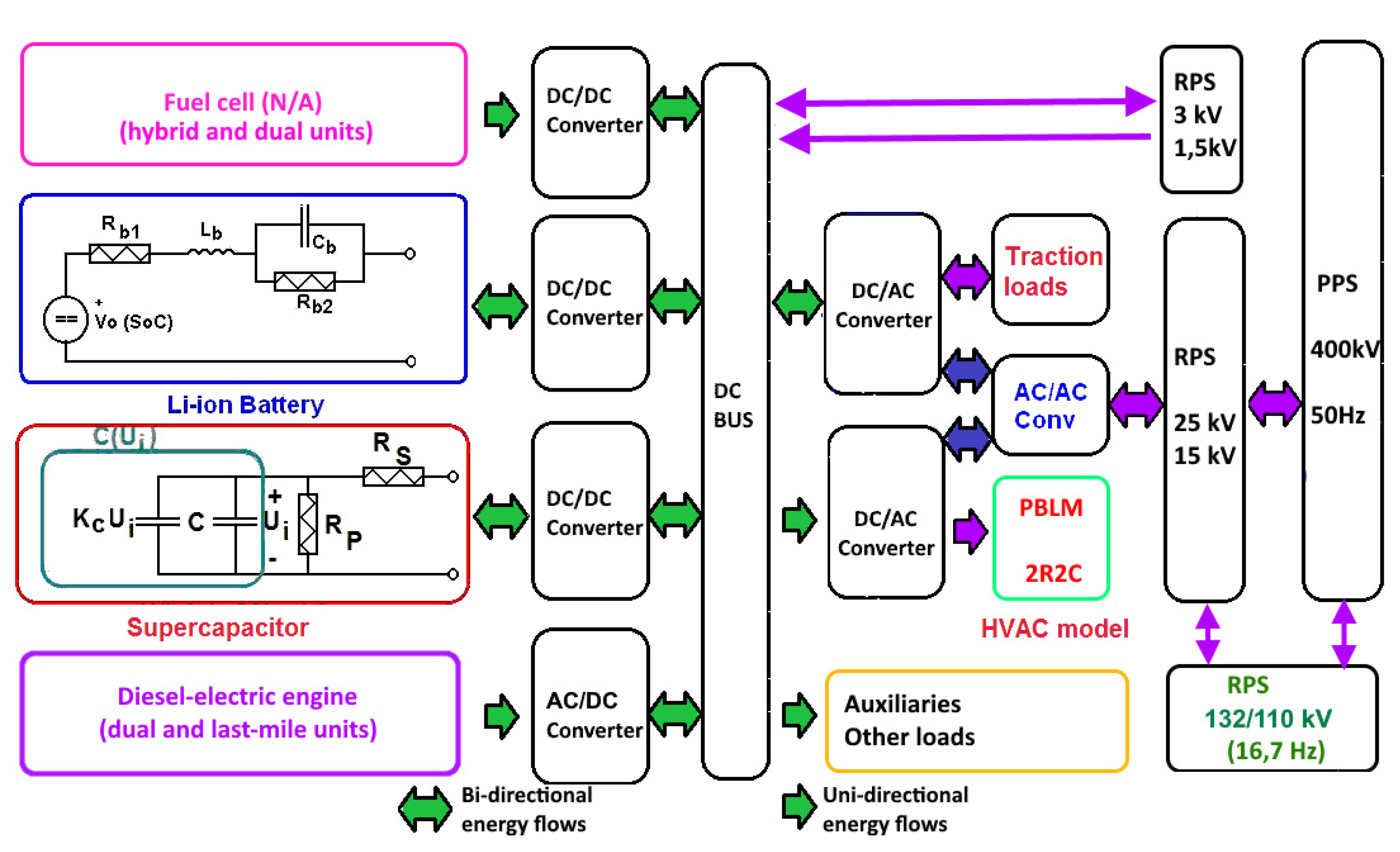
3.2. Integration of Resources in Railway Platforms and Integration of the Simulation Models

Different models have been described in Section 2 (tractive loads and generation, hotel loads, energy storage…) for the simulation of DR policies. Figure 10 shows a picture of how the distinct parts of a train interact with RPS and PPS. The core of this integration is the practical use of a DC bus that makes easier and cheaper the integration of different components (and future concepts) in a railway design and the development of different train families with different capabilities and primary sources (AC/DC supply, diesel-electric, last-mile, dual…) with a minimum change of internal devices through the addition of different modules (for instance, TRAXX [46], VECTRON [47] or Flirt [44] families and, to some extent, Talgo 250 EMU series [40], which has a special interest due to the development and integration of its coaches for many different services in Europe). Figure 10 justifies the mathematical integration of models based on their physical integration to define the overall demand/generation of each train and their flexibility in the DER portfolio.

In this way, hybrid ESS (batteries and supercapacitors, Figure 10) have also been considered for the simulation of “last-mile” options because of their greater flexibility achievable to recover the energy during regenerative braking and for acceleration episodes. This is a main factor in the train arrivals and departures at the terminus station. Moreover, Table 3 depicts that the tractive characteristics of battery EMUs (BEMUs) can be improved with supercapacitors [48] to reach the performance of EMUs in full electric mode, and this is important for fast accelerations required to accomplish timetable performances.

Notice that this regenerative braking is more difficult in DC overhead systems (energy flows in substations are unidirectional) and obviously in non-electrified sections (dual locomotives usually work in those sections) as discussed in [27]. These systems are considered available in power/service car/coaches or in locomotives for simulation purposes. Unfortunately, fuel cells are not considered in this study due to lack of data from manufacturers.

4. Results

4.1. Main Assumptions

This paper entails and simulates the models that have been presented in Section 2 according to the potential resource portfolio supplied by railway manufacturers and described in Section 3. Energy requirements for traction are basic for defining the operation strategies of other resources (i.e., ESS and HVAC loads) according to RPS state. Obviously, demand can be analysed through train simulators, which is a well-known topic in the literature. There are several options available for users; for instance, software packages developed by manufacturers (Sitras by Siemens [49]), research consortiums (CRUISE m by Shif2Rail EU projects [50]) or universities (TrainOps by LKT [51]). Authors have used their own simulator for the models described in Section 2 with the aim to integrate all DER models (Figure 10). It is described in more detail in [27]. According to Table 1 and the characteristics of trains, the power requirements for some conventional trains (IC) and EMU (S, IR, RE) are presented in Figure 11a. It is worth noting that S1 or IR 75 are a type of service, and it does not involve the use of a specific class of locomotive with conventional cars or EMUs. A simulation of the demand in the RPS of Luzern station area, which hypothetically supplies power to our railway timetable scenario, is presented in Figure 11b. The sharp profiles due to acceleration of trains in Figure 11a explain high rates of change in demand, which matches the data reported in [52] for the overall SBB system (up to 25 MW/s).

As stated before, it should be considered that the average life of a locomotive or EMU ranges from 30 to 40 years, and some units remain in service for up to 50 years. Usually, they are refurbished and upgraded several times (every 10–15 years) to meet the expectations of comfort, security, mechanical considerations, and, more recently, environmental constraints due to sustainability scenarios for 2030–2050. These updates benefit the engagement of LM and hybrid options, as discussed in Section 3. For simulation purposes, it is assumed that some trains are new and others are refurbished units, and both include some kind of ESS devices. The success of “TER Regiolis” (SNCF, France) or Cityjet ECO (ÖBB, Austria) prototypes explains their foreseen commercial deployment during 2023–2024. For these refurbished units, the use of commercial battery packs used in electric buses (or ultracapacitors packs from tramways [40]) seems more reasonable, sustainable and cheaper options [31] than the purchase of new units. Nevertheless, many other trains are older units without ESS or additional diesel-electric generators.

Some characteristics of the locational demand curve (Figure 11b) deserve a reflection. First, it is highly possible that two accelerations (and braking) from different units overlap in the time. This can be because speed limits in the departures progressively increase when trains leave the station, and this entails several accelerations to reach cruise speed in the main track. Moreover, delays in timetable can change those overlaps (3–4 min are usually foreseen and tested during timetables planning [5] to account for contingency management). In our simulation scenario, overlaps in demand produce peaks around 6 MW (at the beginning of the hour “1X”, Figure 11b). Second, there are significant time intervals with departures but without arrivals, and vice versa, during each hour. For instance, lack of arrivals from 1X:07 to 1X:15 or from 1X:32 to 1X:41, or the lack of departures from 1X:39 to 1X:54 (see Table 1 and Figure 11b). This last fact involves that some braking energy is difficult to be recovered (without ESS), especially if the energy is supplied by DC catenary and there is not any reversible substation (a common problem due to the higher cost of reversible substations). These remarks drive the simulations in the next sections.

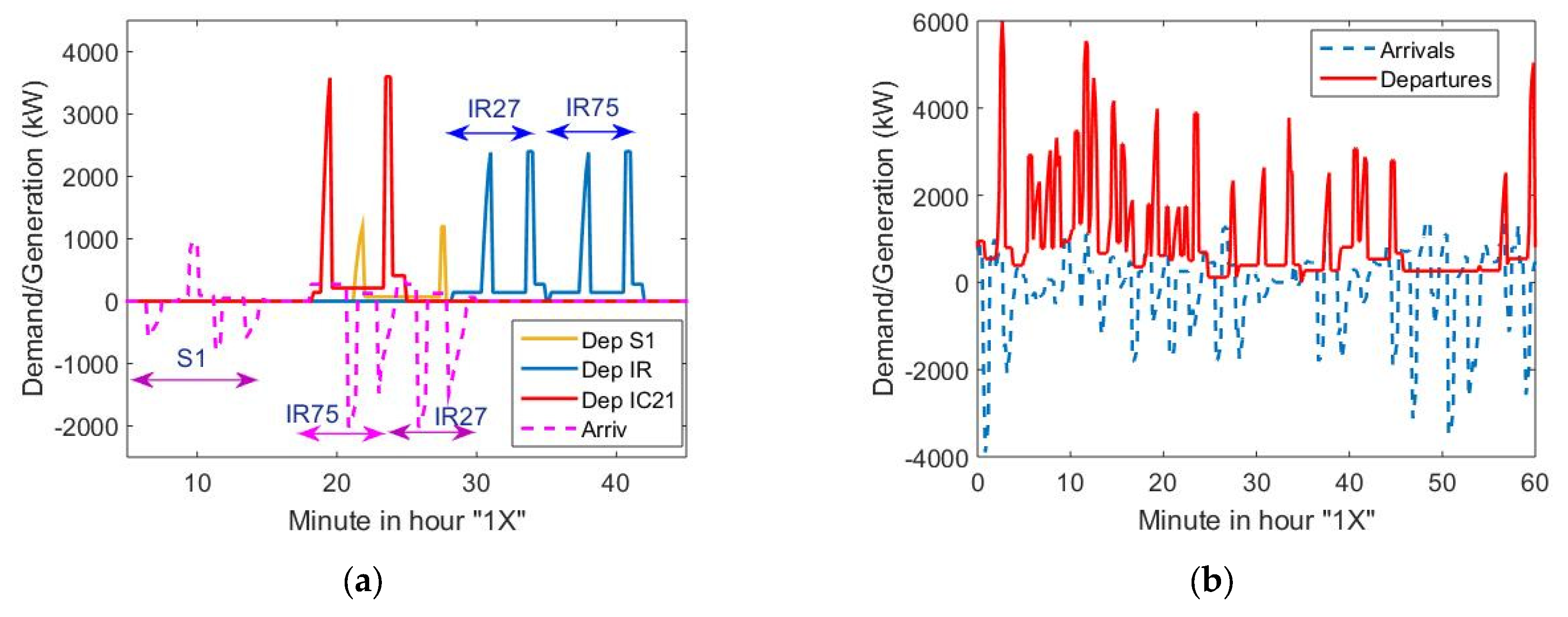
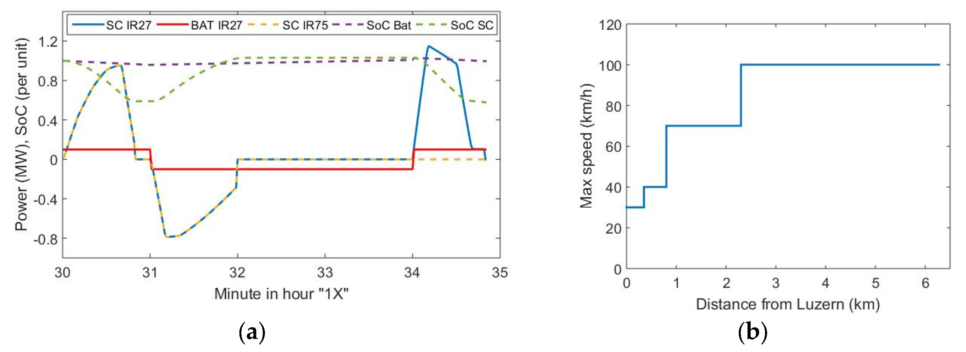
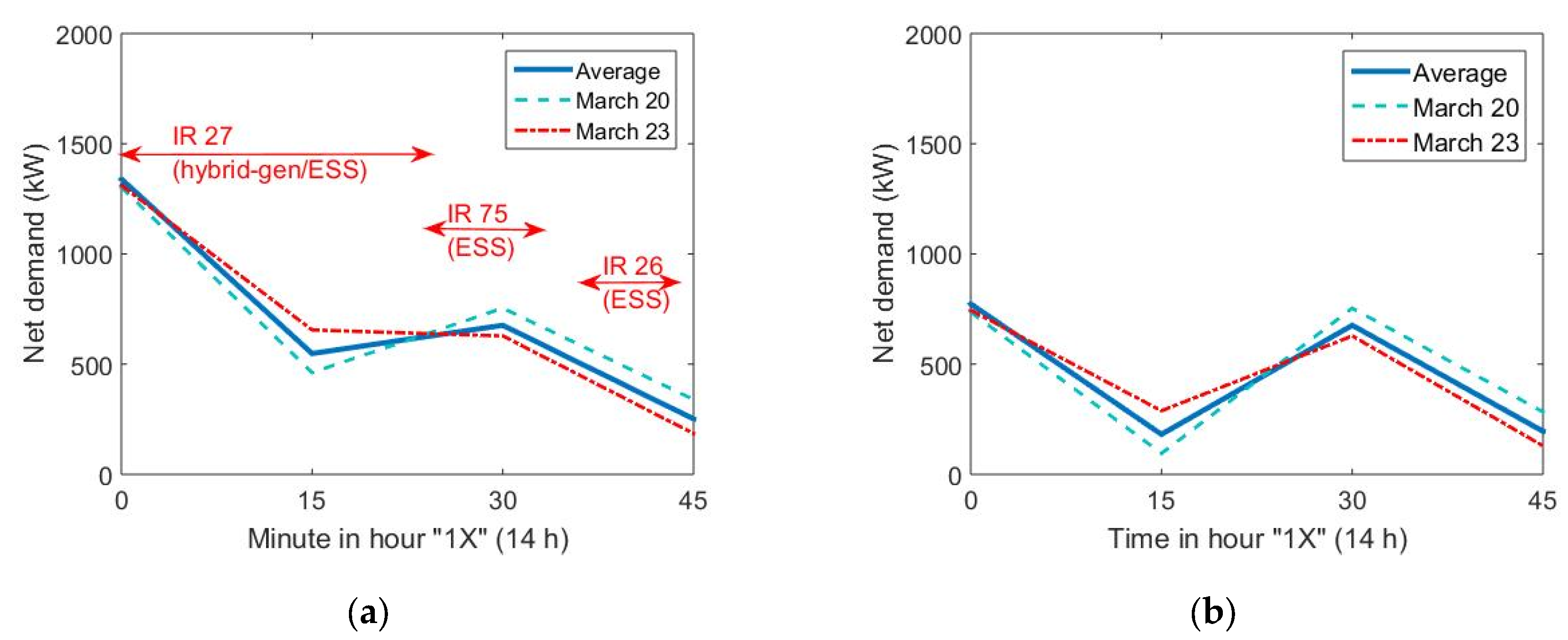
4.2. Potential of Energy Storage Systems

To explain the management of ESS resources (SC and battery), the IR 27 service has been chosen (Figure 4a and Table 1), leaving Luzern at 1X:28 (IR 27). The arrival of S1 and IR 75 (both are different physical units) have generated around 30–40 kWh of braking energy to be recovered by SC banks and, to a minor extent, by Li-ion batteries of the IR 27 (awaiting its departure at 1X:28, Figure 11a, red dashed) and IR 75 (leaving at 1X:35, Figure 11a, red dashed). The energy requirements of these trains are given in

Table 4. Regenerative energy (braking) in arrivals and energy needed for acceleration in departures in Figure 11a.

Arrivals			Departures
Service	Time	Braking Energy (kWh)	Service	Time	Acceleration Energy (kWh)
IR 75	1X:25	31.3
IR 27	1X:30	42.7	IR 27	1X:28	41.8
S4	1X:32	24.7	IR 75	1X:35	45.5

. As stated before, these accelerations explain the sharp peaks and valleys in the demand of the RPS station (Figure 11b). Notice that the success in the operation of both EES, and to a minor extent, HVAC (paragraph 4.4), will partially shave these peaks, and consequently, the need for new AC/AC converters in the RPS (whose price ranges 600–900 EUR /kW) and some auction for energy bids in day-ahead and intraday markets by railway operators (energy aggregators).

To store the energy generated through braking and fulfil the energy requirements for the departure of trains, it is proposed to install a Hybrid-ESS (HESS): an SC around 6 kWh and a 100 kWh bank of batteries in each train (to avoid discharges > 50% in batteries to increase their lifetime). The SC’s target is to cover the high peaks of power needed to accelerate, while batteries can supply the energy necessary for low accelerations and to maintain cruise speed. The optimization of ESS is not considered, and authors follow the size proposed by manufacturers in prototypes (Table 3). Some specific methods can be found in the bibliography [53]. The management of storage devices is depicted in Figure 12.

The proposed strategy is due to the acceleration requirements of train IR 27 when leaving the terminus station at 1X:28 pm. It is assumed that energy recovered through braking (IR 75, IR, and S4) enables the recharge of SCs in units IR 26 and 75 (they are parked in the station, note that the IR 75 unit arriving at Luzern is not the same IR 75 unit staying at the station). When IR 27 leaves, SC and batteries of IR 75 and 27 support its acceleration. Figure 12a depicts that this train accelerates in several steps (according to speed profiles, Figure 12b): the first between 30 km/h to leave the platform and station track points, and then to accelerate to 70 km/h in the common main line; then the second acceleration episode to reach 100 km/h on the specific line to its destination. Figure 12a depicts the power generated by SCs and batteries from IR 27 and 75 and the State of Charge (SoC) of both elements. Ultracapacitors support the main energy needs of IR 27. Fortunately, another IR is braking (punctuality is a benchmark of operator’s quality) and fills both SCs. Once SoC recovers the value 1 (100%), the IR 27 can accelerate until 100 km/h (Figure 12a, at 34 min). In this case, IR 75 does not support generation anymore.

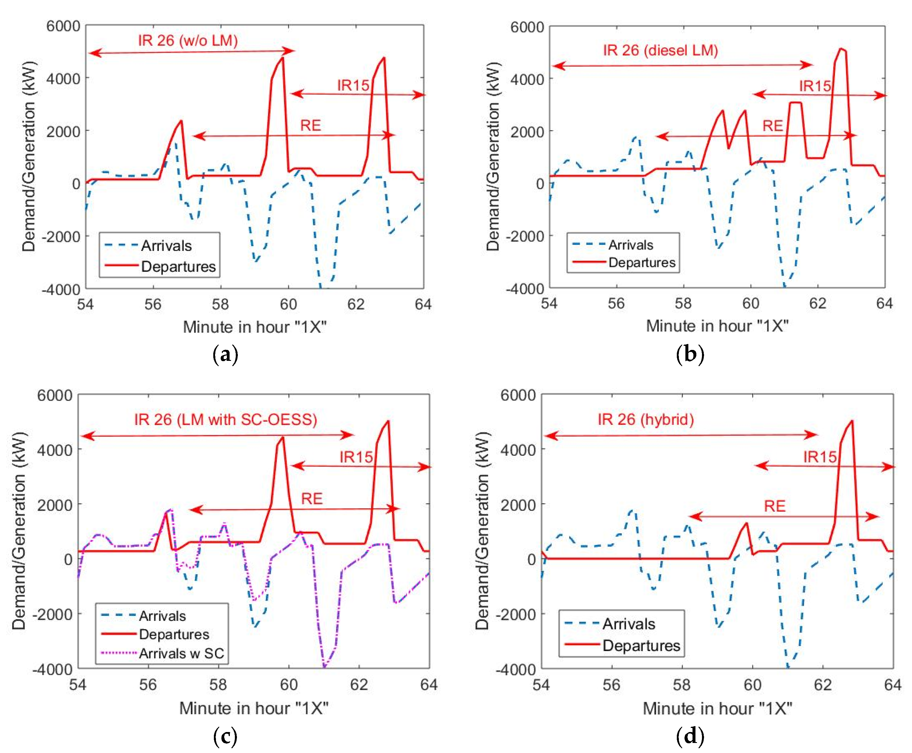
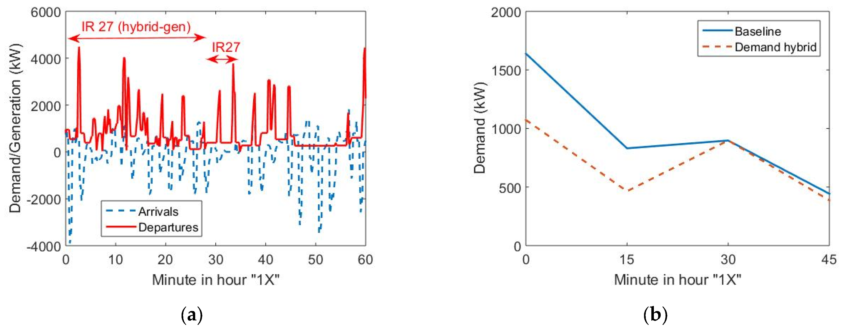
4.3. Potential for Hybrid/Dual Units

Section 3 has discussed two commercial possibilities for LM engines: first, the present available option from main manufacturers is a small-diesel motor (250–400 kW); and then, full-electric (FELM) with on-board ESS (the commercial service is foreseen by 2023–24 [41,45]). Figure 13a depicts the IR and RE energy requirements for “conventional” units (i.e., without LM). Several overlaps during acceleration episodes between trains can be seen and, consequently, produce sharp demand peaks. The main issue in this case is shaving peaks through available LM options.

Figure 13b presents the first option: a locomotive with a small-diesel LM option (used for freight) that hauls IR 26. The IR starts in diesel mode to leave the station and its yard (30 km/h). With this lag, IR 26 can recover (regenerative braking) some more energy from other units (minute 59), then IR 26 unit changes to full electric mode, but the problem here is that the speed of IR 26 is very low (30–35 km/h) and a congestion is possible in the block between IR 26 and a later service (notice that another RE is leaving the station at 1X:57, Table 1). Signal distances (home and routing) are important in this case (perhaps 1–1.5 km). To avoid these constraints, this option is not considered feasible.

The second case depicts a unit with hybrid ESS (HESS) in charge of IR 26. This option reduces the first peak (min 56–57), but the second peak remains (minute 60, Figure 13a), see Figure 13c. In this case, the advantage is that braking energy can be used more efficiently (dashed line in Figure 13c that reduces the overall demand).

Finally, another option is that IR 26 (again a DHEMU) generates up to 2.4 MW from its diesel plants as a distributed generator instead of remaining in standby (platform 4, from 1X:02 as IR 15 to 1X:28, Table 1). This option can present problems, from an environmental point of view, but it can be of interest from an energy point of view. Another possibility is to use a diesel shunting or freight units (updated with a pantograph and AC/AC converters [11]) out of the station in the external yard to limit environmental problems. Several countries, and especially Spain, have lots of diesel-electric freight locos out of service that can be refurbished for this duty. The result of this option is depicted in Figure 14a. The highest peak due to IC train (6.6 MW) is shaved during this hour and in other peak hours (IC21 for this hour, from 14 to 15h). If the unit is equipped with an OESS, the flexibility can be significantly improved because the train endows the main DER options.

Obviously, the driver’s pattern of each train (these patterns can be changed through driving advisory systems [16]) or train delays can modify the scenarios depicted in Figure 13 and Figure 14. The volatility of results should be considered in the future through the automatization of switch between locomotives or EMU modes of traction. A less “volatile” analysis can be undertaken considering the 15-min demand curve (i.e., the transaction period in some energy markets [23]). Demand curve also presents high oscillations, and it becomes a problem for energy management [54]. Interesting solutions are proposed and implemented in [4]. Figure 14b depicts some results for the baseline (for non-flexible units, Figure 11b) and the dual hybrid (DHEMU) option. Obviously, damping is lower when some energy storage and on-site generation is available.

Table 5. Overall results for LM and dual EMU options.

Indicator	Small Diesel LM	Hybrid SC and Battery	Dual Unit	Dual Full Generation	HVAC Control	Baseline
Demand (MWh)	1.34	1.346	1.27	1.11	1.25	1.36
Energy recovery (MWh)	1.16	1.18	1.12	0.96	1.09	1.19
Energy recovery (%)	13	12.2	11.7	13.2	12.7	12
Demand peak (MW)	6.64	6.64	6.64	5.14	6.51	6.64

also depicts some indicators.

It is worth noting that a similar result in peak demand shaving can be achieved with the use of two FELM units (e.g., IR 70 and S1) as explained in Figure 12a and Figure 13c.

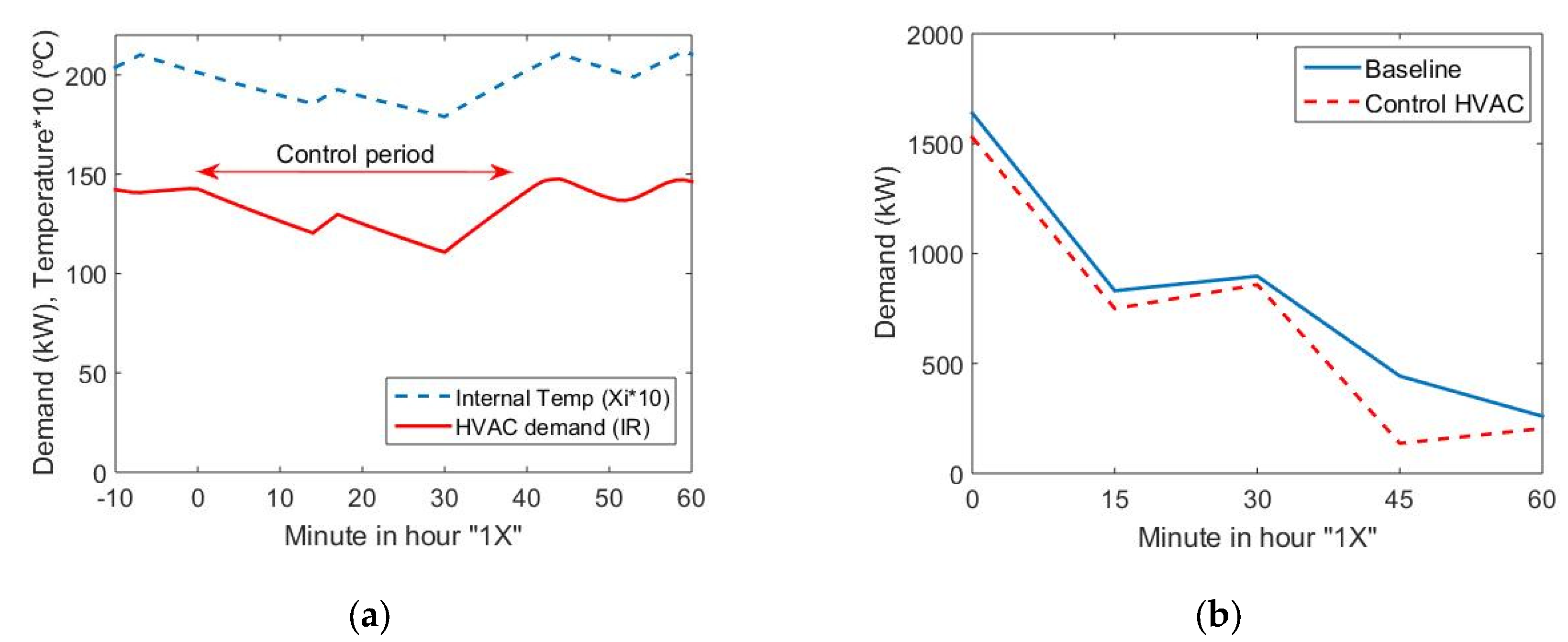
4.4. Management of “Comfort/Hotel” Train Loads

To improve the synergy between DR policies, HVAC demand of trains, leaving or arriving at the station, can be controlled to save up to 20–25% of ancillary demand requirements for 20–45 min (considering the average time of units in the Luzern area) according to the control policy depicted in Figure 15a. Notice that the temperature of coaches with this control remains above 18 °C (Figure 15a) and customer comfort is guaranteed. The contribution to overall peak savings is very small with this DR policy (100–150 kW), but it can be of interest considering the 15-min demand curve (Figure 15b) from the point of view of PPS requirements and energy unbalance (to be discussed in next subsection).

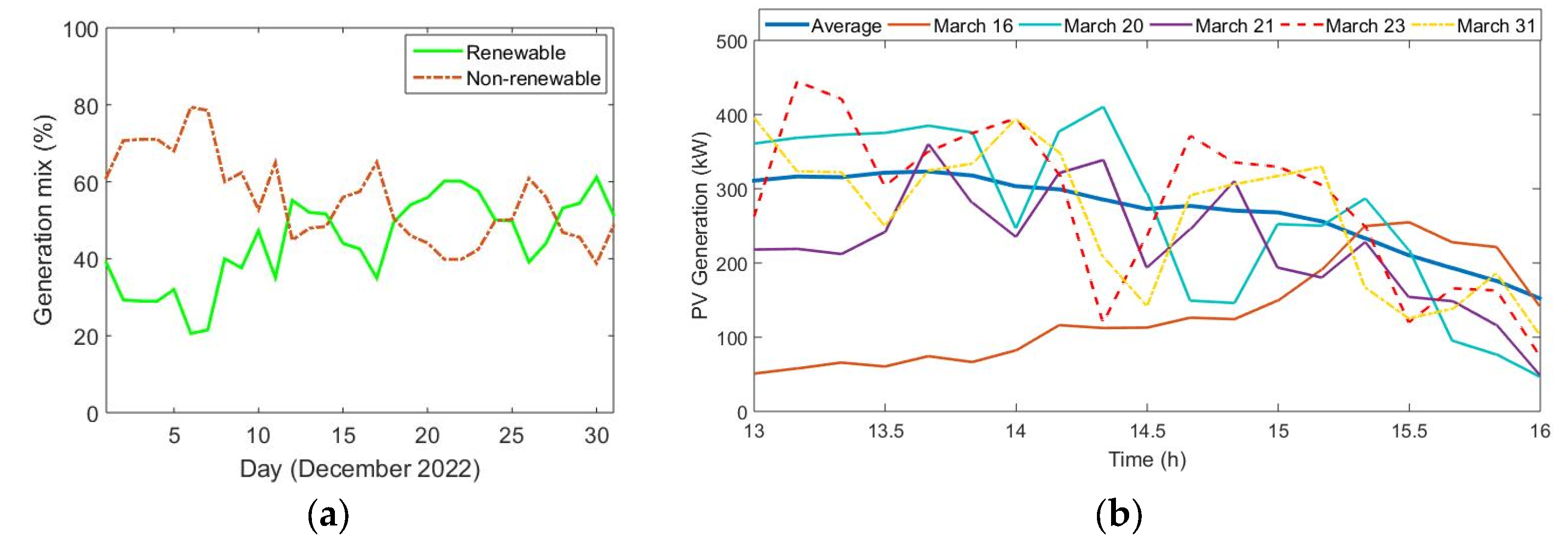
4.5. Integration of Renewables: Potential of Railway Flexible Resources

Renewables are a main pillar of achieving credible sustainability and solving energy concerns in the horizon 2030–2050. The increasing trend of renewable capacity share in the overall generation mix can be seen around the world. The main problem with renewables (wind and photo-voltaic) is that their contribution is highly volatile throughout the year, month, or day. A good example could be seen in Spain in December 2022 (Figure 16a). As can be seen, the integration of renewables must be supported by conventional sources (the traditional approach of the “supply side”) or through a higher response on the demand side. This last option requires the development and engagement of new flexible resources with new “abilities”.

In this subsection, it is assumed that a photovoltaic generation plant is installed near the railway station. Its rated power is 500 kWp and a railway operator, or another agent, owns and manages this plant. Figure 16b shows the average generation in March 2019 and some hourly curves (in the same period used for simulation purposes in this section).

This PV plant helps in shaving demand peaks (from the point of view of the PPS). Figure 17a shows the 15-min demand curve (now a net demand curve) for the Luzern system, without the participation of any flexible resource (see Figure 14b for comparison purposes) for the monthly average PV generation and two different days. Obviously, the net demand is reduced, but the problem remains from the point of view of RPS (power oscillations and peaks in short time periods, i.e., minute to minute).

Moreover, the volatility of renewables on March 20, with respect to March 23, presents a problem from the point of view of energy balancing because the (railway) operator will be responsible for its own balance in the near future. A plausible solution is the development of short-term generation models (day-ahead) for PV, but as discussed by the authors in [55], this is a complex task and an additional model (very short term, i.e., hour ahead) is needed, but it does not limit errors. Let us assume that this day-ahead model works fine for regular days (close to the average curve in Figure 16b), but it is necessary to reduce the error in balance (an additional cost for operators) through very short-term models.

Let us consider that the hour-ahead model fits the daily curves (March 20 and 23). We can use flexible railway resources to fix the unbalance due to the errors of day-ahead forecasting models, which are models used to buy energy in electricity markets. As can be seen in Figure 17a, the unit charge of IR 27, IR 75, and IR 26 services are available again in the flexibility portfolio during different time intervals that cover around 90% of the target time for balancing. The strategy is similar to the one presented in Figure 14: IR 27 supplies power with its diesel plant, and IR 75 and IR 26 are also in an “alert” state to balance forecast errors in PV generation (i.e., net demand foreseen by hour-ahead model) through their ESS capacity. From the curve depicted in 17a, the railway operator needs to balance up or down around 100 kW in two 15-min intervals (15–30 and 30–45 min), i.e., IR 75 and IR 26 need 25 kWh of storage to fit PV error forecasts (this is, 25% of their ESS capacity) and, in this way, to avoid unbalances (and penalties). Figure 17b depicts some results due to the operation of IR 27 (dual EMU) in the PPS 15-min net demand curve. The conclusion is that both power systems (PPS and RPS) reduce their peaks by 25% and are balanced at PPS levels even through the integration of renewable generation.

4.6. Some Economic Considerations

From an economic point of view, up to 1.5 MW can be clipped in the Luzern area RPS during peak periods (Table 5) with two FELM units (or with a DHEMU). Specific cost for battery of EUR 120–130/kWh is considered for this evaluation, and a specific cost of EUR 11,000–12,000/kWh for SCs. The engagement of ESS systems in EMUs can reduce the size of AC/AC inverters that link RPS and PPS (e.g., around EUR 700/kW, including BoS [56]). In addition, the operator avoids the need to purchase energy in balance (a main concern for RPS in the future) or intraday markets (e.g., around EUR 50–150/MWh). With respect to units, authors estimate that six trains that operate in these services need to include ESS systems on board.(HESS). Results are shown in

Table 6. Cost and benefits of HESS and HVAC control configuration (10 years).

Technology and Capital Cost (kEUR)	Peak Reduction (kW)	Cost (kEUR)	Energy Reduction (MWh/yr)	Benefit (kEUR)
ESS, SC (6 units) and 120 SC modules (1)	1300	430	262	26.2
ESS, battery (6 units) and 100 kWh	150	720	1200	120
HVAC control (40 EMU)	150	100	100	10
AC/AC 50/16.7 Hz inverter (1 unit)	1600			1100
Energy in short-term markets	-		45	4.5

⁽¹⁾ 48 V and 165 F [48].

, and the proposal is near cost-effectiveness at this pre-feasibility level.

It is worthing to note again that service requests of train operators have some tolerances in timetable settings, and this can be used to optimize demand and energy costs during the planning process of next year’s timetables. For example, DB Netz AG (Germany) apply “design tolerances” of ±3 min for passenger services. Another significant input to define the flexibility of train loads is punctuality limits. In the Swiss railway system, this limit is set at 3 min [5]. Both factors should be carefully considered from an energy point of view and need a full stochastic approach in the next research developments.

5. Conclusions

This paper entails and simulates how the introduction of new technologies in railways, mainly explained by decarbonization and sustainability policies, can afford the application of new resources and policies in Power Systems. Energy Storage, Mobile Distributed Generation and Demand Response, which are similar to conventional DER in PPS, have been identified and simulated for RPS to improve the implementation of periodic timetables. The use of flexible resources reduces the stress of current infrastructures, allowing the lagging of new resources and the introduction of storage in electric and diesel units, which limits environmental impacts and improves energy efficiency through an increase in regenerative braking (10% in the simulation scenario). To perform this objective, physical-based train models (locomotives and EMUs with LM options), “hotel/comfort load”, and ESS models have been revisited and linked to improving the usefulness of simulation results. Braking energy can therefore be harvested by ESS, and energy efficiency is improved both in RPS and PPS. Moreover, the use of load management (during time dwellings) and ESS avoids, to some extent, the problems related to the high ramps experienced by demand in RPS systems because of periodic timetables. In conclusion, the proposed policies in the simulation scenario achieve around a 25% reduction in peak demand and around a 30% reduction in demand fluctuations considering the 15-min demand curve (RPS and PPS). Moreover, the paper demonstrates that flexible railway resources can have an interesting potential in balancing the unpredictability of renewable generation (photovoltaic), in this case, enabling balance strategies foreseen in the future development of energy markets.

The achievable flexibility of railway loads discussed in this work can also be used in the integration of renewables with Public Power Systems through the enlargement of responsible customer segments. Finally, these alternatives appear cost-effective considering the cost of ESS with respect to the cost of locomotives and EMUs, and this result can catalyse the increase in the share of railway transportation in the EU and other countries (for passengers but also for freight services). It is worth noting that the proposed alternatives have considerable synergies in railway systems with partially electrified routes or many different voltages and frequencies (e.g., Europe), where the presented alternatives provide some additional advantages to ESS systems and their management.

Obviously, the problem of planning timetables is very complex, but the management of demand must be considered as a main factor, and this new flexibility can provide new opportunities to reduce potential issues dealing with the implementation of periodic timetables.

References

1. International Railways Union (UIC), “Technologies and Potential Developments for Energy Efficiency and company CO2 Reductions in Rail Systems”. 2016. Available online: https://uic.org/sustainability/energy-efficiency-and-co2-emissions/ (accessed on 6 December 2022).
2. Bahn 2000—Mehr Zug Für Die Schweiz (Rail 2000 Initiative, More Railway for Switzerland). Available online: https://www.admin.ch/gov/fr/accueil/documentation/communiques.msg-id-1161.html (accessed on 15 November 2022).
3. SBB-CFF-FFS. Swiss Railway Operator Web Page. Available online: http://www.sbb-cff-ffs.ch (accessed on 31 August 2022).
4. Load Management—Smart Grid at SBB. Available online: https://company.sbb.ch/en/sbb-as-business-partner/services-rus/energy/load-management.html (accessed on 28 July 2019).
5. Graffagnino, T. Managing Timetable Risks. 2019. Available online: https://ethz.ch/content/dam/ethz/special-interest/dual/riskcenter-dam/Seminar%20Series/Slides/191022_TimetableRisksGraffagnino_01.pdf (accessed on 29 September 2022).
6. Demand Response Web Page. Available online: http://www.demandresponse.eu (accessed on 25 October 2022).
7. Agency for Railways (European Union), “Fostering the Railway Sector Through the European Green Deal”. 2020. Available online: https://www.era.europa.eu/content/report-fostering-railway-sector-through-european-green-deal_en#oe-content-oe-documents (accessed on 30 November 2022).
8. Europe’s Rail Joint Undertaking (EU-Rail), “Work Programme 2022-24. Draft Amendment n 2”. Available online: https://rail-research.europa.eu/wp-content/uploads/2022/09/AWP_2022_AMEMDMENT_final_20220909.pdf (accessed on 6 December 2022).
9. Zawadzki, A.; Resweski, F.; Pahl, M.; Schierholz, H.; Burke, D.; Vasconcellos, B.; Toppan, M. “Riding the Rails to Sustainability”, Boston Consulting Group (BCG) Report, February 2022. Available online: https://www.bcg.com/publications/2022/riding-the-rails-to-the-future-of-sustainability (accessed on 20 November 2022).
10. Raghavan, S.V.; Wei, M.; Kammen, D.M. Scenarios to decarbonize residential water heating in California. Energy Policy 2017, 109, 441–451. [Google Scholar] [CrossRef]
11. Agenjos, E.; Gabaldon, A.; Franco, F.G.; Molina, R.; Valero, S.; Ortiz, M.; Gabaldon, R.J. Energy Efficiency in Railways: Energy Storage and Electric Generation in Diesel Electric Locomotives. In Proceedings of the CIRED 2009– 20th International Conference and Exhibition on Electricity Distribution, Prague, Czech Republic, 8–11 June 2009; pp. 1–7. [Google Scholar] [CrossRef]
12. BLS AG (Railway Operator). Available online: https://www.bls.ch/en (accessed on 31 October 2022).
13. Schweizerische Südosbahn AG (Railway Operator). Available online: https://www.sob.ch/ (accessed on 31 October 2022).
14. Die Zentralbahn. Available online: https://www.zentralbahn.ch/en (accessed on 12 October 2022).
15. The SBB Timetable. Available online: https://www.sbb.ch/en/timetable.html (accessed on 15 October 2022).
16. Energy Efficient Timetabling at SBB, Energy Efficient Time Tabling Workshop, 20 Feb. 2018, Brussels. Available online: https://uic.org/events/IMG/pdf/006_energy_efficient_timetabling_sbb_p.keiser.pdf (accessed on 29 September 2022).
17. Wang, Y.; Li, D.; Cao, Z. Integrated timetable synchronization optimization with capacity constraint under time-dependent demand for a rail transit network. Comput. Ind. Eng. 2020, 142, 106374. [Google Scholar] [CrossRef]
18. Caimi, G.; Kroon, L.; Liebchen, C. Models for railway timetable optimization: Applicability and applications in practice. J. Rail Transp. Plan. Manag. 2017, 6, 285–312. [Google Scholar] [CrossRef]
19. Herrigel, S.; Laumanns, M.; Nash, A.; Weidmann, U. Hierarchical Decomposition Methods for Periodic Railway Timetabling Problems. Transp. Res. Rec. J. Transp. Res. Board 2013, 2374, 73–82. [Google Scholar] [CrossRef]
20. Restel, F.; Haładyn, S.M. The Railway Timetable Evaluation Method in Terms of Operational Robustness against Overloads of the Power Supply System. Energies 2022, 15, 6458. [Google Scholar] [CrossRef]
21. Urbaniak, M.; Kardas-Cinal, E. Optimization of Train Energy Cooperation Using Scheduled Service Time Reserve. Energies 2022, 15, 119. [Google Scholar] [CrossRef]
22. Transpotrail WebMagasin. Le Cadencement: L’horlogerie Ferroviaire Suisse. Available online: http://transportrail.canalblog.com/pages/le-cadencement---l-horlogerie-ferroviaire-suisse/39243719.html (accessed on 13 September 2022).
23. PEEXPORT. Center Market Data. Available online: https://www.epexspot.com/en/extras/download-center/market_data. (accessed on 15 October 2022).
24. Allenbach, J.-M.; Chapas, P.; Comte, M.; Kaller, R. Traction Électrique; Presses Polytechniques et Universitaires Romandes: Lausanne, Switzerland, 2008; ISBN 2880746744. [Google Scholar]
25. Wu, Q.; Spiryagin, M.; Cole, C. Train energy simulation with locomotive adhesion model. Rail. Eng. Science. 2020, 28, 75–84. [Google Scholar] [CrossRef]
26. Ogawa, T.; Manabe, S.; Yoshikawa, G.; Imamura, Y.; Kayegama, M. Method of Calculating Running Resistance by the Use of the Train Data Collection Device. Q. Rep. RTRI 2017, 58, 21–27. [Google Scholar] [CrossRef]
27. García-Garre, A.; Gabaldón, A. Analysis, Evaluation and Simulation of Railway Diesel-Electric Units as Distributed Energy Resource. Appl. Sci. 2019, 9, 3605. [Google Scholar] [CrossRef] [Green Version]
28. Rochard, B.P.; Schmid, F. A review of methods to measure, Lausanneand calculate train resistances. Proc. Inst. Mech. Eng. Part F J. Rail Rapid Transit 2000, 214, 185–199. [Google Scholar] [CrossRef]
29. Wu, Q.; Wang, B.; Spiryagin, M.; Cole, C. Curving resistance from wheel-rail interface. Veh. Syst. Dyn. 2022, 60, 1018–1036. [Google Scholar] [CrossRef]
30. Wu, Q.; Yang, X.; Jin, X. Hill-starting a heavy haul train with a 24-axle locomotive. Proc. Inst. Mech. Eng. Part F J. Rail Rapid Transit. 2022, 236, 201–211. [Google Scholar] [CrossRef]
31. Voith Web Page: Rail Vehicles. Available online: https://voith.com/cn/1728_e_g_2180_e_rb_maxima_sgl_2010.pdf (accessed on 25 October 2022).
32. Vitins, J. New Electric Locomotives for the UK: TRAXX UK with Last Mile Feature, The 20th Annual Rail Freight Group Conference, May 2012, London (UK). Available online: https://www.qca.org.au/wp-content/uploads/2019/06/10088_r-bombadiernewelectriclocomotivesfortheukthe20thannualrailfreightgroupconference-submission-qrnetworketsdaau-1012.pdf (accessed on 25 October 2022).
33. Spiryagin, M.; Wu, Q.; Wolfs, P.; Sun, Y.; Cole, C. Comparison of locomotive energy storage systems for heavy-haul operation. Int. J. Rail Transp. 2018, 6, 1–15. [Google Scholar] [CrossRef]
34. García-Garre, A.; Gabaldón, A.; Álvarez-Bel, C.; Ruiz-Abellón, M.D.C.; Guillamón, A. Integration of Demand Response and Photovoltaic Resources in Residential Segments. Sustainability 2018, 10, 3030. [Google Scholar] [CrossRef]
35. Rail Tec Arsenal Fahrzeugversuchsanlage, Wien, Austria. Available online: https://www.rta.eu/en/ (accessed on 9 June 2022).
36. Zhang, L.; Hu, X.; Wang, Z.; Sun, F.; Dorrell, D.G. A review of supercapacitor modeling, estimation, and applications: A control/management perspective. Renew. Sustain. Energy Rev. 2018, 81, 1868–1878. [Google Scholar] [CrossRef]
37. Sustrail Research Project (7th EU Framework Research Programme). Hybrid Locomotive Report. 2019. Available online: https://www.sustrail.eu/IMG/pdf/d3.2-v1-hybrid_locomotive-final_version.pdf (accessed on 24 October 2022).
38. Mazzone, A.; Schönbacher, M.; Larrea, X. Future Freight Locomotives in Shift2Rail-Development of Full Electric Last Mile Propulsion System. In Proceedings of the 7th Transport Research Arena TRA 2018, Vienna, Austria, 16–18 April 2018. [Google Scholar]
39. Brenna, M.; Foiadelli, F.; Stocco, J. Battery Based Last-Mile Module for Freight Electric Locomotives. In Proceedings of the 2019 IEEE Vehicle Power and Propulsion Conference (VPPC), Hanoi, Vietnam, 14–17 October 2019; pp. 1–6. [Google Scholar] [CrossRef]
40. Patentes Talgo, S.A. High Speed Talgo 250 Dual. Available online: https://www.talgo.com/250-dual (accessed on 12 October 2022).
41. SNCF Innovation and Research. Regiolis Hybrid BEMU. Available online: https://www.sncf.com/en/innovation-development/innovation-research/hybrid-ter-coming-soon-to-station-near-you (accessed on 15 November 2022).
42. Saft Batteries. Available online: https://www.saftbatteries.com/media-resources/press-releases/saft-battery-systems-provide-ideal-board-backup-power-package-caf%E2%80%99s (accessed on 1 September 2022).
43. Fedele, E.; Iannuzzi, D.; Del Pizzo, A. Onboard energy storage in rail transport: Review of real applications and techno-economic assessments. IET Electr. Syst. Transp. 2021, 11, 279–309. [Google Scholar] [CrossRef]
44. Standler Rail. Flirt Akku BEMU. Available online: https://www.stadlerrail.com/en/flirt-akku/details/ (accessed on 15 November 2022).
45. ÖBB Cityjet Eco. The First Certified Battery-Powered Train in Europe. Available online: https://www.oebb.at/dam/jcr:b697320b-4493–48f2-a9f4-b8ff3af4d4ec/datenblatt-cityjet-eco.pdf (accessed on 15 November 2022).
46. ALSTOM Rolling Stock Solutions: TRAXX Family Locomotives. Available online: https://www.alstom.com/traxx-locomotive-superior-performance-every-environment (accessed on 15 November 2022).
47. Siemens Mobility Solutions: VECTRON Locomotives. Available online: https://www.mobility.siemens.com/global/en/portfolio/rail/rolling-stock/locomotives.html?gclid=Cj0KCQiA37KbBhDgARIsAIzce15BqM1TsWOEy-6us6E4UJtVK9ET8_-1lGO7T-RJIwOEu3mALKoazcwaAiSIEALw_wcB&acz=1 (accessed on 25 October 2022).
48. Maxwell Technologies. Ultracapacitors for Railway Applications. Available online: https://maxwell.com/products/ultracapacitors/48v-module-with-durablue/ (accessed on 3 November 2022).
49. Siemens, A.G. System Design with Sitras Sidytrac Simulation of AC and DC Traction Power Supply. Available online: https://assets.new.siemens.com/siemens/assets/api/uuid:ad3c8251-2b8b-464b-bda3-26a416368c2f/siemens-sidytrac-pi-en.pdf. (accessed on 1 September 2022).
50. Shift2Rail Initiative. Available online: https://rail-research.europa.eu/about-shift2rail/ (accessed on 15 November 2022).
51. LTK Engineering Services. TrainOps. Available online: https://www.ltk.com/trainops#excellence (accessed on 14 June 2019).
52. Feldmann, R.L. Time-Optimized Power Consumption: Towards a Smart Grid for Rail Infrastructure. Available online: https://www2.vpe.hu/document/6297/SBB_Raimund%20Feldmann_Time-optimized%20power%20consumption_Towards%20a%20smart%20grid%20for%20rail%20infrastructure.pdf (accessed on 1 September 2022).
53. Kapetanović, M.; Núñez, A.; van Oort, N.; Goverde, R.M. Reducing fuel consumption and related emissions through optimal sizing of energy storage systems for diesel-electric trains. Appl. Energy 2021, 294, 117018. [Google Scholar] [CrossRef]
54. Feldmann, R.L.; Fuchs, A.W. From Energy Management to Power Management, Global Railway Review, Issue 6. 2017. Available online: https://www.globalrailwayreview.com/article/63589/energy-management-power-management/ (accessed on 5 October 2022).
55. Ruiz-Abellón, M.C.; Fernández-Jiménez, L.A.; Guillamón, A.; Falces, A.; García-Garre, A.; Gabaldón, A. Integration of Demand Response and Short-Term Forecasting for the Management of Prosumers’ Demand and Generation. Energies 2020, 13, 11. [Google Scholar] [CrossRef] [Green Version]
56. Fu, R.; Remo, T.; Margolis, R.U.S. Utility-Scale Photovoltaics-Plus-ESS Costs Benchmark. NREL/PR-6A20–72401 Report. Available online: https://www.nrel.gov/docs/fy19osti/71714.pdf (accessed on 10 October 2022).
Figure 1. The definition process of railway timetables considering electricity demand and its costs.
Sustainability 15 02746 g001
Figure 2. An example of a Sankey diagram for the approximate use of energy in railways.
Sustainability 15 02746 g002
Figure 3. An example of a diagram for a partial nodal point with 00 and 30 symmetries in Luzern timetable (notice that not all services follow this symmetry, for example IC-21 and S1). Arrows define arrivals (entering the clock numbers) and departures (leaving the clock numbers) of the service.
Sustainability 15 02746 g003
Figure 4. SBB-CFF-FFS System: (a) Demand and generation mix covering demand adapted from [4]; (b) Some examples of EPEX day-ahead prices (2021 and 2022).
Sustainability 15 02746 g004
Figure 5. Effort characteristics of different vehicles considered for simulation (null values indicate that the locomotive/unit cannot reach this speed): (a) Tractive effort for conventional locomotives (manufactured or rebuilt from 1992 to 2020), (b) Tractive effort for locomotives with “Last Mile” options by Bombardier, TRAXX LM (freight version, in service in EU equipped with a small diesel unit) and for a dual hybrid diesel and electric multiple unit (DHEMU) by Patentes Talgo S.A, Spain.
Sustainability 15 02746 g005
Figure 6. Nominal voltage in overhead railway systems (catenary) in main European countries and some examples of freight corridors (yellow arrows) that justify the use of diesel-electric units for some passenger and freight services.
Sustainability 15 02746 g006
Figure 7. Auxiliary end-uses (in kW) for a second-class car (B10t standard coach 26.40 m length, 44 t). Rated power: 45 kVA. Ratio of demand: 500–550 W/passenger.
Sustainability 15 02746 g007
Figure 8. PBLM model of HVAC loads corresponding to passenger coaches used in the paper: (a) Representation of the thermal model and the different subsystems considered for a railway vehicle; (b) A two resistor and two capacitor (2R2C) electric–thermal equivalent network used in the modelling process (subsystems or sub-models 1–3).
Sustainability 15 02746 g008
Figure 9. Results from PBLM tractive models: (a) Measurement and simulation speeds (TS is a train stop in this service, MT is a temporary speed limits due to maintenance works that is near the maximum height of the itinerary); (b) Characteristics of the stretch.
Sustainability 15 02746 g009
Figure 10. PBLM models for ESS to be used in the paper for simulation purposes (equivalent ultra/super-capacitor and equivalent battery) and their interaction with other models (traction and HVAC loads) and with RPS and PPS.
Sustainability 15 02746 g010
Figure 11. Individual and aggregated demand and generation: (a) Demand for acceleration and generation through regenerative braking for some trains leaving and arriving from minute 10 to minute 40 in hour “1X” according to Table 1. (b) Generation and Demand profiles for the hour “1X”.
Sustainability 15 02746 g011
Figure 12. Strategies for ESS resources: (a) Demand profiles and SoC considered for simulation at Luzern station; (b) Maximum speeds considered for simulation (from Luzern).
Sustainability 15 02746 g012
Figure 13. Strategies for railway DER resources applied to some services in hour “1X”: (a) baseline: demand and generation without DER; (b) change in demand patterns with an LM locomotive hauling IR 26 (small diesel engine) (c) change in demand pattern with FELM (IR 26); (d) change in demand patterns with a dual hybrid unit in charge of service IR 26.
Sustainability 15 02746 g013
Figure 14. Strategies for DER resources: (a) hourly demand and generation with IR 27 engaged as generator; (b) 15-min demand with and without DER availability.
Sustainability 15 02746 g014
Figure 15. Strategies for HVAC loads in IR units: (a) 20–25% of load cycle reduction; (b) Impact of HVAC load reduction in 15-min demand curve.
Sustainability 15 02746 g015
Figure 16. Examples of renewable generation: (a) Share of renewables in the overall Power System (example: Spain, December 2022); (b) Hourly profiles (around hour “1X”) for PV generation in March 2019 (capacity 500 kWp).
Sustainability 15 02746 g016
Figure 17. Examples of balance management through flexible railway resources: (a) Baseline and time availability for each resource; (b) Management of net demand through IR 27 (dual unit with onboard generation).
Sustainability 15 02746 g017