Abstract
The prediction of air pollutants has always been an issue of great concern to the whole of society. In recent years, the prediction and simulation of air pollutants via machine learning have been widely used. In this study, we collected meteorological data and tropospheric NO2 column concentration data in Beijing, China, between 2012 and 2020, and compared the two methods of time sequence-based and influencing factor-based random forest regression in predicting the tropospheric NO2 column concentration. The results showed that prediction of the tropospheric NO2 column concentration using random forest regression was affected by the changes of human activities, especially emergency events and policy variations. The advantage of time sequence analysis lies in its ability to calculate the distribution of air pollutants with a long-time scale of prediction, but it may produce large errors in numerical value. The advantage of influencing factor prediction lies in its high precision and that it can identify the specific impact of each influencing factor on the NO2 column concentration, but it needs more data and work quantities before it can make a prediction about the future.
1. Introduction
With the development of industries, air pollution has become a problem of increasing concern and aroused widespread attention from the whole of society. Nitrogen oxides are the main air pollutants and are directly or indirectly related to atmospheric environment problems, such as photochemical smog, acid deposition and stratospheric ozone depletion, among others [1,2,3]. NO2 is the main component of nitrogen oxides in the atmosphere, and its monitoring and prediction can, to a greater extent, serve as a guide to the control of atmospheric nitrogen oxides and therefore help formulate policies for their emission, reduction and control. Large numbers of mathematical and machine-learning models have been developed to calculate and describe the distribution and change of atmospheric NO2. Weather research and prediction in combination with the weather research and forecasting community multiscale air quality modeling system (WRF-CMAQ) and weather research and forecasting-chemistry (WRF-Chem) have been used extensively [4,5,6]. Shin et al. (2018) [7] made a linear regression analysis of NO2 in Japanese metropolises using the spatiotemporal random tree model and found that it was advantageous to use this model to simulate spatiotemporal changes of NO2. Zhan et al. (2018) [8] established a new model known as random forest space-time Kriging (RF-STK) and used it to assess the exposure risks of NO2 and SO2 in some regions of China.
The most critical issue in the management of air pollution is the prediction of the concentration and distribution of the pollutants, and air pollution cannot be controlled by only analyzing the pollution that has occurred. Moolchand et al. (2021) [9] established a modified model of extrapolating air pollutants based on historical and current meteorological datasets and calculated the results from 196 cities in India on various classifiers, finding that the accuracy of linear robust regression was 94–96%. This accuracy could be improved to some extent after using various types of clustering algorithms, showing that the optimal accuracy of the decision-tree classifier was 99.7%, and the use of the random forest classifier could raise the accuracy by 0.02%, indicating that the accuracy of machine-learning algorithms is superior to that of the linear model in predicting air pollutants. Sriram et al. (2021) [10] predicted the air quality index (AQI) in Delhi by using the decision tree, support vector machine (SVM), naive Bayes classifier, logistics regression, random forest and K-nearest neighbor as the supervised machine-learning algorithms, finding that the decision tree method produced the best results with an overall accuracy of 99.8%. The results of the prediction models, based on big data analysis and machine learning, can help assess the current air quality and compare the assessments. In the present study, we established a NO2 column concentration distribution prediction model based on the random forest regression mainly by using the time sequence analysis and influencing factor prediction methods with the purpose of compare their advantages and disadvantages of the two methods and their respective application settings. Wang et al. [11] used TROPOMI and HRRR data to develop a random forest model of ozone to estimate ground-level ozone concentrations in California. This model allows the contribution of satellite data products to be assessed in a concise modelling framework, and their findings suggest that TROPOMI data improve the estimation of extremes in ground-level ozone modelling. It could also accelerate future research on the application of satellite data products and high-resolution meteorological data to predict ground-level ozone concentrations. Long et al. [12] developed models for estimating daily ground-level NO2 in China using four tree-based machine learning models (decision tree (DT), gradient boosted decision tree (GBDT), random forest (RF) and extra tree (ET)), and found that the estimated high-resolution results were consistent with ground-based observations of NO2 through spatio-temporal analysis and comparison, and that of the four models, the extra-tree model with the spatio-temporal information (based on the ST-ET) model outperformed the remaining three models for the 2019 estimation. This is, in addition, to the large number of studies based on tree models, which demonstrate the generalizability of tree-based machine learning models for atmospheric pollution studies at a global scale.
Much of the past research exists in the discussion of studies of one or several different models. Rarely has there been an analysis of different ideas and approaches to one model. Moreover, in the traditional use of machine learning models, the results of a single model are mostly used as a conclusion. In contrast to previous studies, we discuss two commonly used methods for prediction and analysis based on random forest regression models (RFR). The advantages, disadvantages and applicability of both methods are investigated, while we also provide a more detailed quantitative analysis of the relationship between influencing factors and atmospheric pollutants as an extension to the random forest regression model.
In a study by Rui F et al. (2019) [13], it was shown that machine learning takes less than one percent of the computation time of the traditional atmospheric models. Simulating hours of seven air pollutants for 4 months in 2018 using WRF-based would take more than 6 days. The same data would take less than 1 h for machine learning using a personal laptop with four cores. Considering that the random forest model has a faster computing speed and lower technical requirements than other models, such as the WRF and neural network models, it is more suitable for social communication. Therefore, we choose the random forest regression model for our research discussion.
Beijing is a world-famous ancient capital and modern international city, as well as the capital and the political, economic and cultural center of China, located in the north of China and North China Plain, adjacent to Tianjin in the east and Hebei in the west with the center at 116°20′ E and 39°56′ N (Figure 1).
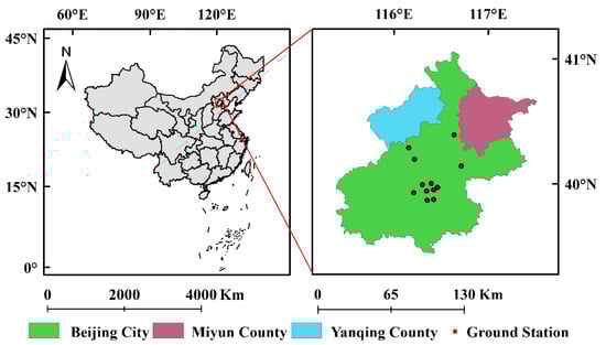
Figure 1.
Brief description of the situation in Beijing, China.
Geographically, Beijing is high in the northwest and low in the southeast; its west, north and northeast sides are surrounded by mountains, and the southeast side is a plain gently inclining to the Bohai Sea. The climate of Beijing belongs to the warm temperate semi-humid and semi-arid monsoon climate, hot and rainy in summer and cold and dry in winter.
As the capital of China, Beijing is the city that responds most promptly to policy and is also the earliest to monitor air pollutants in China. The changes in air pollutants in Beijing are representative of most major cities in China.
2. Data and Methods
2.1. Data Sources
Satellite data were obtained from the ozone monitoring instrument (OMI) aboard NASA’s Aura satellite (https://disc.gsfc.nasa.gov/ (accessed on 15 October 2021)) [14]. In the present study, we used the product of OMI/Aura NO2 tropospheric column L3global grid 0.25 × 0.25 degrees V3. As this product has undergone data filtration and only preserves the cloud fraction data <30%, it is unnecessary to do additional filtration. In addition, hourly real-time monitoring data of air quality released by the National Urban Air Quality Real-time Publishing Platform of China’s Environmental Monitoring Station were used (http://www.cnemc.cn/ (accessed on 15 October 2021)). The data used in this study were the mean daily value calculated from NO2 data per hour.
Using the re-analysis data released by the National Centers for Environmental Prediction (NCEP)/National Cholesterol Education program/National Center for Atmospheric Research (NCAR) (https://psl.noaa.gov/data/gridded/data.ncep.reanalysis.html (accessed on 15 October 2021)) and the lifted index selected (LI, °C) from it, tropospheric temperature (K), atmospheric pressure (Pa), precipitable water volume (PWV, kg/m2) and relative humidity (RH%) were calculated.
2.2. Methods
In the Python Sklearn random forest regression module, the max depth determined the downward frequency of the decision trees: the deeper the max depth, the more accurate the fitting result. However, excessive max depth may result in excessive fitting. The number of trees determines the size of the random forest model: the more trees, the more accurate the result obtained [15]. The random number determines the occurrence of events. If there is no specified random number, each calculation would produce a different result, and therefore the specified random number can help the client find better hyperparameters. The learning curve of the drawn model indicates that an excessively complex model will reduce the accuracy of the model, meaning that the excessive number of trees and excessive depth will increase the time of calculation and reduce the accuracy of the model. For this reason, accurate selection of the hyperparameter can greatly increase the accuracy and speed of the random forest model (Figure 2).
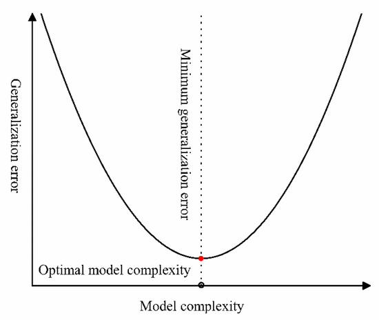
Figure 2.
Learning curve of the random forest regression model.
Based on the above knowledge, three main hyperparameters are required to establish a random forest: the number of decision trees to be produced (n_estimator), the depth of the tree model (max_depth) and the random number (random_state) [16].
In this study, we used Python GDAL, Pandas, Numpy, Scipy, Sklearn and Jupyter modules to treat data and generate images, among which the GDAL module has great power in calculating grid images. In this study, we used GDAL to read raster in raster calculation followed by matrix operation. To ensure the accuracy of the model and the occurrence of excessive fitting, we selected the hyperparameter R2 score less than 0.98 to establish the model.
The time sequence prediction model was established by selecting the NO2 column distribution for n successive year as the target value of NO2 concentration distribution of tag value n + 1 year, and training was performed on it to obtain the optimal hyperparameters. Using the trained model, we predicated the NO2 concentration of n + 2 years and obtained good prediction results.
As no grid images representing large numbers of human activity data were available, especially industrial and traffic data, and only monthly or yearly mean data were available, we only selected part of the meteorological data as influencing data in establishing the influencing factor prediction model in this study, which does not mean that these are the only influencing factors.
Prediction models using influence factors, due to the large amount of human activity data, especially industrial and traffic data, do not exist as raster images, only monthly average or annual average data, so this paper only selects some meteorological data as influence factors. This paper only discusses the scenarios of using two methods and does not analyze the NO2 column concentration in the study area in depth, so the influence factors selected are only those that can make the model established and relatively accurate.
The model R2 and RMSE shown in this paper are only for the training set, and the RMSE for the predicted data set is discussed in detail in the paper.
Figure 3 shows the flow diagram for the adjustment of the model parameters used in this paper.
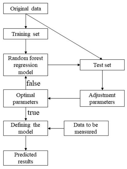
Figure 3.
Workflow diagram.
3. Results and Discussion
3.1. Changes of the Tropospheric NO2 Column Concentration in Beijing from 2012 to 2020
As shown in Figure 4, the NO2 column concentration in the target areas decreased gradually yearly from 2012 to 2020, the highest mean value being 17.49 ± 2.80 × 10¹⁵ molec/cm2 in 2012 and the lowest mean value being 7.80 ± 1.66 × 10¹⁵ molec/cm2. This was cumulatively and similar to the observations of Chi et al. in 2021 [17]. Compared with 2014, the NO2 column concentration in 2013 decreased significantly, mainly because of the publication of the “Action Plan of Prevention and Control of Air Pollution” in China during 2013 and 2014 [18]; the main elements are the strengthening of the treatment of air pollutants, the limitation of air pollutant emissions, the requirement to use clean energy, the use of clean technology, the improvement of the monitoring system and the establishment of an early warning system, etc. [19].
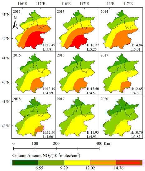
Figure 4.
Distribution of the tropospheric NO2 column concentration in Beijing, China between 2012 and 2020 (Annual average value).
3.2. The Time Sequence Prediction Model
As air pollutants present a typical seasonal distribution, it is necessary to establish corresponding models of calculation according to the different months. We selected March, June, September and December to establish the model and used the NO2 column concentration data from 2012 to 2019 to predict the NO2 column concentration in 2020. The data engineering and prediction results are presented in Model 1/Table 1 and Figure 5/Table 2, respectively.

Table 1.
Data engineering of the 2020 NO2 column concentration prediction model (x for month).

Figure 5.
Error distribution between the result obtained by the NO2 column concentration model and the actual result obtained by OMI in 2020.
Table 2.
Result error of 2020 NO2 column concentration prediction.
As shown in Figure 5 and Table 2, the error of the result, obtained by Model 1, was relatively great, especially for the results obtained in March and December, in which the maximum error was 40.4% and 61.53%, respectively. Considering the outbreak of COVID-19 pandemic in 2020, human activities may be greatly limited by the pandemic outbreak. To verify this hypothesis, we established a prediction model to predict the NO2 column concentration in 2019. The data engineering and prediction results are presented in Model 2/Table 3 and Figure 6/Table 4, respectively.
Table 3.
Data engineering of the 2019 NO2 column concentration prediction model (x for month).
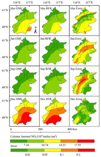
Figure 6.
Error distribution between the result obtained by the NO2 column concentration model and the actual result obtained by OMI in 2019.
Table 4.
Result error of 2020 NO2 column concentration prediction.
As shown in Figure 6 and Table 4, Model 2 was superior to Model 1, especially in the result error; the maximum error appeared in March 2019, being 30.65%. As shown in the distribution map, the error exceeded 20% in only a few areas. The mean error of the four months was less than 10%, and the maximum root mean square error (RMSE) of the four months was 6.71%. The prediction result of the NO2 column concentration distribution was more accurate as compared with Model 1. These results confirmed the hypothesis that human activity changes in 2020 had a great impact on the time sequence-based prediction model. Other than emergency events, policy variations also had a huge impact on human activities and air pollutant emission.
Given the great policy variations in 2014, the data engineering and result of the 2019 NO2 column concentration prediction model based on 2014–2018 are shown in Model 3/Table 5 and Figure 7/Table 6, respectively.
Table 5.
Adjusted data engineering of the 2019 NO2 column concentration prediction model (x for month).
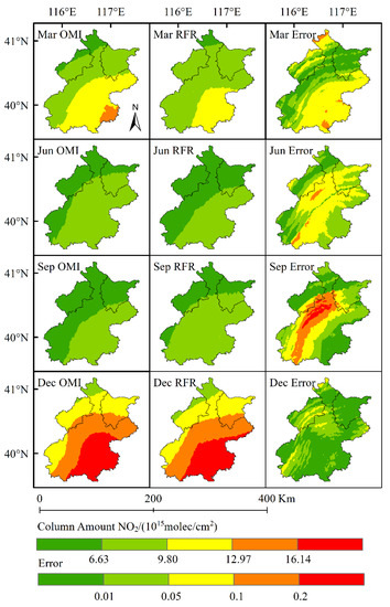
Figure 7.
Error distribution between the result obtained by the adjusted NO2 column concentration model and the actual result obtained by OMI in 2019.
Table 6.
Results error of adjusted 2019 NO2 column concentration prediction.
As shown in Figure 7 and Table 6, the error of Model 3 was smaller than that of Model 2. The maximum RMSE of the four months appeared in March 2019, being 5.39%. The RMSE of the root mean square error of the four months was less than 5%, except March 2019. All other results of Model 3 were superior to Model 2. Knowing that the higher the learning frequency, the better the prediction result (theoretically, the more the characteristic years, the better the prediction result in principle), the phenomenon that Model 3 was superior to Model 2 demonstrates that the time sequence-based prediction model by taking into consideration the human activities or emission policy variations is better than that without considering the human activities or emission policy variations. In addition, fewer months means faster calculation, indicating that policy variations and limitations on human activities should be considered when time-sequence prediction is performed. Although the prediction error was relatively high in some target areas when time sequence was used to predict the NO2 column concentration, its result of NO2 column concentration distribution is acceptable.
The accuracy has been significantly improved compared to traditional models [6,17]. A comparison of the previous studies using machine learning models found that the precision of our estimates was similar to the results of other studies, but slightly lower than that of similar studies that introduced other influencing factors [11,12].
3.3. Prediction of Influencing Factors
The model established based on the meteorological factors and NO2 column concentration from 2014 to 2018 alone was unable to predict the NO2 column concentration in 2019, and therefore data from the ground monitoring stations were added. The data engineering (Model 4/Table 7) and results are shown in Table 8.
Table 7.
Data engineering of the influencing factor-based NO2 column concentration prediction model.
Table 8.
Result of the influencing factor-based NO2 column concentration prediction model.
As shown in Table 8, the result error was smaller than that of the time-sequence-based prediction model (Model 2/3) and the prediction result was closer to the actual value. However, the NO2 concentration data obtained from the ground monitoring stations in 2019 were required during model establishment. As a result, it could only predict the pollution events that had occurred. If the time sequence-based prediction model was first used to predict the meteorological data followed by using the predicted data obtained to predict the pollutants, the error would be increased.
The method has predictive power and is more accurate than traditional studies [20,21]. The accuracy of the predictions is similar to previous studies using machine learning methods [16]. If the data obtained from the ground monitoring stations were used to predict tropospheric NO2 column concentration, the result would to some extent lose its predictive meaning, because the predicted air pollutants have occurred at the time of prediction. Model 4 is more similar to an inverting model. The influencing factor-based prediction model is able to obtain the impact of each influencing factor on the NO2 column concentration within the time interval in the target area via the importance interface and identify which influencing factor produces the greater impact on the NO2 column concentration. The results are listed in Table 9.
Table 9.
Important parameters of the influencing factor-based NO2 column concentration prediction model.
Figure 8 is the partial dependence plot (PDP) of the impact of each influencing factor on the NO2 column concentration in March 2019 by using the important parameters obtained through the importance interface. By using this PDP and multiple linear regression, we can establish the conditional function relationship specific to air pollutants.
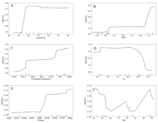
Figure 8.
Partial dependence plot between various influencing factors and the NO2 column concentration obtained by Mode 4 using random forest regression. (A): the NO2 concentration obtained by the ground monitoring station; (B): precipitable water volume; (C): tropospheric temperature; (D): lifted index selected; (E): atmospheric pressure; (F): relative humidity.
The results are normalized results. As there are not enough data when is located in 32.98~37.23, we were unable to establish the functional relationship.
: tropospheric NO2 column concentration; : tropospheric temperature, : LI; : PWV; : atmospheric pressure; : RH; : ground monitoring station NO2 concentration.
The results of the calculation of the No2 column concentration for March 2019 based on the obtained functional relationship are shown in Figure 9. It can be seen that the results are very close to the measured values of OMI with a trend line slope of 0.96 R2 of 0.96 RMSE of 0.34 × 10¹⁵ molec/cm2. It can be proved that the obtained functional relationship can describe the relationship between the influencing factors and the NO2 column concentration.
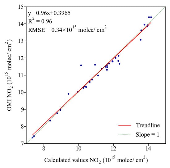
Figure 9.
Comparison of the results calculated from the functional relationship with the measured values of OMI.
The above demonstrates that the result displayed by the functional relationship calculated by multiple linear regression is somewhat different from that calculated by RFR, especially in the ordination of PWV and tropospheric temperature, mainly due to the following reasons: (1) the relationship between NO2 and the influencing factors is complex and not simply a linear relationship, and therefore the multiple linear regression model can only partially reflect good fitting; (2) the 32.98~37.23 interval is lost, but this is the interval in which the greatest change may occur; (3) the concentration range of the NO2 concentration released by the ground monitoring stations is not clearly defined. The cause may be that classification of the concentration range needs sufficiently large data in each range to ensure the accuracy of the result obtained by the multiple linear regression model. Finer classification of concentration ranges often means less data in each range; it is usually difficult to control this conflict point because it is liable to make an a priori judgement to obtain a better functional relationship, which is unacceptable to result analysis. The relationship between various influencing factors and the NO2 column concentration needs to be further explored in future research.
The limitations of the modeling approach discussed in this paper can be avoided by selecting more detailed and richer impact factors, e.g., Brokamp et al. (2018) [22] and Hu et al. (2017) [23] developed a daily pm2.5 prediction model for the U.S., using data mainly including AOD, meteorology and land use. Predictions based on influencing factors for pollutants, such as NO2, SO2, and O3, can be made by adding local emission data, such as emission inventories, but the time scale of their prediction is short and it is difficult to achieve long-time scale prediction. We will conduct research in this area in subsequent studies.
4. Conclusions
- Human activities and emission policy variations should be taken into full consideration in using the time sequence-based air pollutant RFR model. Although the result obtained by this model is not accurate enough, it can be used to predict air pollutant distributions and has the positive significance for governments or enterprises in formulating pollutant emission policies.
- The influencing factor-based air pollutant RFR prediction model is more accurate than the time sequence-based air pollutant RFR model in predicting pollutant concentrations, but it is unable to predict the overall pollutant distributions. It needs a large and complex amount of work to select influencing factors and perform data processing. Regardless it can calculate the impact of each influencing factor on air pollutants. It is therefore of great significance in analyzing the specific impact of each influencing factor on air pollutants.
Author Contributions
All authors contributed to the study conception and design. Conceptualization, methodology were performed by T.J. Software, validation, formal analysis, writing—original draft were performed by T.G. and B.L. Writing—review and editing, data curation, visualization were performed by B.A. and H.S. All authors have read and agreed to the published version of the manuscript.
Funding
This work was supported by the National Natural Science Foundation of China (2016YFC0500907) and the Natural Science Foundation of Gansu Province (CN) (17YF1FA120) at the Key Laboratory of Resource Environment and Sustainable Development of OasisGansu Province.
Institutional Review Board Statement
We declare that we do not have human participants, human data or human issue.
Informed Consent Statement
Not applicable.
Data Availability Statement
The data and Python code that support the findings of this study are openly accessible on request.
Conflicts of Interest
The authors have no relevant financial or non-financial interests to disclose.
References
- Carmona-Cabezas, R.; Gómez-Gómez, J.; Gutiérrez de Ravé, E.; Jiménez-Hornero, F.J. Checking complex networks indicators in search of singular episodes of the photochemical smog. Chemosphere 2020, 241, 125085. [Google Scholar] [CrossRef] [PubMed]
- Fan, H.; Zhao, C.; Yang, Y. A comprehensive analysis of the spatio-temporal variation of urban air pollution in China during 2014–2018. Atmos. Environ. 2020, 220, 117066. [Google Scholar] [CrossRef]
- Xie, Z.; Du, Y.; Zeng, Y.; Li, Y.; Yan, M.; Jiao, S. Effects of precipitation variation on severe acid rain in southern China. J. Geogr. Sci. 2009, 19, 489–501. [Google Scholar] [CrossRef]
- An, X.; Zhu, T.; Wang, Z.; Li, C.; Wang, Y. A modeling analysis of a heavy air pollution episode occurred in Beijing. Atmos. Chem. Phys. 2007, 7, 3103–3114. [Google Scholar] [CrossRef]
- Xu, R.; Tie, X.; Li, G.; Zhao, S.; Cao, J.; Feng, T.; Long, X. Effect of biomass burning on black carbon (BC) in South Asia and Tibetan Plateau: The analysis of WRF-Chem modeling. Sci. Total Environ. 2018, 645, 901–912. [Google Scholar] [CrossRef] [PubMed]
- Shen, Y.; Jiang, F.; Feng, S.; Zheng, Y.; Cai, Z.; Lyu, X. Impact of weather and emission changes on NO2 concentrations in China during 2014–2019. Environ. Pollut. 2021, 269, 116163. [Google Scholar] [CrossRef] [PubMed]
- Araki, S.; Shima, M.; Yamamoto, K. Spatiotemporal land use random forest model for estimating metropolitan NO2 exposure in Japan. Sci. Total Environ. 2018, 634, 1269–1277. [Google Scholar] [CrossRef] [PubMed]
- Zhan, Y.; Luo, Y.; Deng, X.; Zhang, K.; Zhang, M.; Grieneisen, M.L.; Di, B. Satellite-Based Estimates of Daily NO2 Exposure in China Using Hybrid Random Forest and Spatiotemporal Kriging Model. Environ. Sci. Technol. 2018, 52, 4180–4189. [Google Scholar] [CrossRef] [PubMed]
- Sharma, M.; Samyak, J.; Sidhant, M.; Hussain, S.T. Forecasting and Prediction of Air Pollutants Concentrates Using Machine Learning Techniques: The Case of India. IOP Conf. Ser. Mater. Sci. Eng. 2021, 1022, 012123. [Google Scholar] [CrossRef]
- Yarragunta, S.; Nabi, M.; Jeyanthi, P.; Revathy, S. Prediction of Air Pollutants Using Supervised Machine Learning. In Proceedings of the 2021 5th International Conference on Intelligent Computing and Control Systems (ICICCS), Madurai, India, 6–8 May 2021; pp. 1633–1640. [Google Scholar] [CrossRef]
- Wang, W.; Liu, X.; Bi, J.; Liu, Y. A machine learning model to estimate ground-level ozone concentrations in California using TROPOMI data and high-resolution meteorology. Environ. Int. 2022, 158, 106917. [Google Scholar] [CrossRef] [PubMed]
- Long, S.; Wei, X.; Zhang, F.; Zhang, R.; Xu, J.; Wu, K.; Li, Q.; Li, W. Estimating daily ground-level NO2 concentrations over China based on TROPOMI observations and machine learning approach. Atmos. Environ. 2022, 289, 119310. [Google Scholar] [CrossRef]
- Feng, R.; Zheng, H.-J.; Gao, H.; Zhang, A.-R.; Huang, C.; Zhang, J.-X.; Luo, K.; Fan, J.-R. Recurrent Neural Network and random forest for analysis and accurate forecast of atmospheric pollutants: A case study in Hangzhou, China. J. Clean. Prod. 2019, 231, 1005–1015. [Google Scholar] [CrossRef]
- Nickolay, A.; Krotkov, L.N.; Lamsal, S.V.; Marchenko, E.A.; Celarier, E.J.; Bucsela, W.H.; Swartz, J.J.; the OMI Core Team. OMI/Aura NO2 Cloud-Screened Total and Tropospheric Column L3 Global Gridded 0.25 Degree × 0.25 Degree V3, NASA Goddard Space Flight Center, Goddard Earth Sciences Data and Information Services Center (GES DISC); GES DISC: Greenbelt, MD, USA, 2019. [Google Scholar] [CrossRef]
- Breiman, L. Random Forests. Mach. Learn. 2001, 45, 5–32. [Google Scholar] [CrossRef]
- Probst, P.; Wright, M.N.; Boulesteix, A.L. Hyperparameters and tuning strategies for random forest. Wiley Interdiscip. Rev. Data Min. Knowl. Discov. 2019, 9, e1301. [Google Scholar] [CrossRef]
- Chi, Y.; Fan, M.; Zhao, C.; Sun, L.; Yang, Y.; Yang, X.; Tao, J. Ground-level NO2 concentration estimation based on OMI tropospheric NO2 and its spatiotemporal characteristics in typical regions of China. Atmos. Res. 2021, 264, 105821. [Google Scholar] [CrossRef]
- Lu, Z.; Huang, L.; Liu, J.; Zhou, Y.; Chen, M.; Hu, J. Carbon dioxide mitigation co-benefit analysis of energy- related measures in the Air Pollution Prevention and Control Action Plan in the Jing-Jin-Ji region of China. Resour. Conserv. Recycl. X 2019, 1, 100006. [Google Scholar] [CrossRef]
- Central People’s Government of the People’s Republic of China. Action Plan of Prevention and Control of Air Pollution, 2012-9-10. Available online: https://www.gov.cn/zhengce/content/2013-09/13/content_4561.htm (accessed on 1 November 2022).
- Zhang, H.; Wang, Y.; Hu, J.; Ying, Q.; Hu, X.-M. Relationships between meteorological parameters and criteria air pollutants in three megacities in China. Environ. Res. 2015, 140, 242–254. [Google Scholar] [CrossRef] [PubMed]
- Yang, J.; Kang, S.; Ji, Z.; Yin, X.; Tripathee, L. Investigating air pollutant concentrations, impact factors, and emission control strategies in western China by using a regional climate-chemistry model. Chemosphere 2020, 246, 125767. [Google Scholar] [CrossRef]
- Brokamp, C.; Jandarov, R.; Hossain, M.; Ryan, P. Predicting Daily Urban Fine Particulate Matter Concentrations Using a Random Forest Model. Environ. Sci. Technol. 2018, 52, 4173–4179. [Google Scholar] [CrossRef]
- Hu, X.; Belle, J.H.; Meng, X.; Wildani, A.; Waller, L.A.; Strickland, M.J.; Liu, Y. Estimating PM2.5 Concentrations in the Conterminous United States Using the Random Forest Approach. Environ. Sci. Technol. 2017, 51, 6936–6944. [Google Scholar] [CrossRef] [PubMed]
Disclaimer/Publisher’s Note: The statements, opinions and data contained in all publications are solely those of the individual author(s) and contributor(s) and not of MDPI and/or the editor(s). MDPI and/or the editor(s) disclaim responsibility for any injury to people or property resulting from any ideas, methods, instructions or products referred to in the content. |
© 2023 by the authors. Licensee MDPI, Basel, Switzerland. This article is an open access article distributed under the terms and conditions of the Creative Commons Attribution (CC BY) license (https://creativecommons.org/licenses/by/4.0/).