Wind Farm Layout Optimization/Expansion with Real Wind Turbines Using a Multi-Objective EA Based on an Enhanced Inverted Generational Distance Metric Combined with the Two-Archive Algorithm 2

Abstract

In this paper, the Wind Farm Layout Optimization/Expansion (WFLO/E) problem is formulated in a multi-objective optimization way with specific constraints. Furthermore, a new approach is proposed and tested for the variable reduction technique in the WFLO/E problem. To solve this problem, a new method based on the hybridization of the Multi-Objective Evolutionary Algorithm Based on An Enhanced Inverted Generational Distance Metric (MOEA/IGD-NS) and the Two-Archive Algorithm 2 (Two Arch2) is developed. This approach is named (MOEA/IGD-NS/TA2). The performance of the proposed approach is tested against six case studies. For each case study, a set of solutions represented by the Pareto Front (PF) is obtained and analyzed. It can be concluded from the obtained results that the designer/planner has the freedom to select several configurations based on their experience and economic and technical constraints.

1. Introduction

Both energy demand and global warming concerns are rising globally. The best option to deal with this issue is to use green energy sources instead of relying on fossil fuels. As a result, renewable energy sources such as wind are becoming increasingly prevalent worldwide [1]. Despite the significant adverse effects of COVID-19 globally, 93 GW of new wind power capacity was installed in 2020, according to the Global Wind Report-2021 [2] issued by the Global World Energy Council (GWEC). Leading the way in installing wind infrastructure are China and the United States. A total of 743 GW of wind energy capacity is now available globally. According to the paper, this increase in wind energy establishments must be tripled to lessen the effects of global warming. Onshore or offshore wind farms can provide wind energy, but the latter option is far more expensive to develop and run. Onshore wind farms are less expensive and more appropriate for operation than offshore ones. However, one aspect of all types is ensuring the wind farm is designed and planned as effectively as possible [3]. Further, measures must be taken to ensure the sustainability of the installed wind farms [4].

Among the main issues of wind energy research is the arrangement of wind farms or Wind Turbines (WTs) while extracting energy from the resource. The wind farm layout is an optimization problem, inherently non-linear, restricted, and dependent on several variables. Modeling the intermittent wind resource, which hinges on where the installation is made, is among the complex tasks. A poorly designed WT layout hinders operation and undermines the WT’s wake effect concern [5]. A mounted WT’s wakes are connected to other WTs in the layout and disrupt the entire system. Among the optimization problem’s most demanding and computationally complex tasks is the proper simulation of the wake effect. Recently, various wind farms have been proposed, taking into account how to maximize wind farm power while minimizing the wake impact [6]. In addition to the wake effect problem, the optimization problem presents various modeling and management challenges, including wind modeling [7], power curve optimization [8], WT maintenance and up-gradation. As a result, such non-deterministic polynomial problems cannot be solved by traditional optimization techniques. Wind Farm Layout Optimization (WFLO) challenges are increasingly being solved using metaheuristic optimization algorithms.

Most WFLO problem formulations aim to maximize produced energy while minimizing cost and satisfying various limitations. To date, numerous metaheuristic techniques, such as Particle Swarm Optimization (PSO) [9,10], Genetic Algorithm (GA) [11,12], Evolutionary Algorithm (EA) [13] and Simulated Annealing (SA) [14], have been tested on these problems to find the best answer. An EA with several goals was suggested by [15] to address the issue. Numerous WTs were added when formulating the problem in the article [16], and a sophisticated EA was used to find a solution. With the aid of energy capture analysis and wake loss investigation, the accuracy of the suggested method was examined in this research. Another recently developed method was tested in [13] in a formulation that depended on the global cost function and included an initial investment and a cash flow amount. The authors of [17] integrated several methods for mathematical programming to create a greedy heuristic algorithm that resolved the WFLO problem. The Ant Colony Optimization (ACO) [18] was tested with a comparable issue formulation, and the comparison analysis demonstrates that it can outperform the other strategies. The same authors dealt with the WFLO problem with varying wind speeds and directions using a particle filtering algorithm in a different publication [18].

The Most Valuable Player Algorithm (MVPA), a relatively new and effective optimization technique, was used [19] to solve the issue, and the outcomes were remarkably satisfying. A hyper-heuristic optimization problem is used to solve the WFLO problem in [20,21] propose using a Biogeography-Based Optimization (BBO) method to build wind farms with numerous WT installations. The WT layout problem is tested with a different directional restriction-based optimization approach [22] when wind farms are subjected to various wind directions. The article [23] utilized a regression-based neural network to accelerate the Differential Evaluation (DE) technique employed in optimizing WT layout. The optimal hub height has been investigated for Egypt in [24], along with the economic assessment and wind energy potential analysis. In [25], a multi-objective algorithm is used to tackle the simultaneous optimization of two objective functions: cost minimization of the WT installation and maximizing production capacity. Decomposition-based algorithms [26] and pseudo-random number generation-based algorithms [27] both deal with similar issue formulations with two opposing objective functions [27]. The problem of different hub heights was addressed in the works [28,29] and solved using genetic and greedy algorithms, respectively.

Despite its incredibly high computational cost, the authors of [30] have offered a novel method of building the wind farm optimally using Computational Fluid Dynamics (CFD) model software. The Coral Reefs Optimization algorithm with Substrate Layer (CRO-SL), which can combine various search algorithms in a single population, is employed in a fairly recent work [31], which proposes an ensemble strategy for tackling the WFLO issue. In [32], a multi-objective Elitist Teaching–Learning Based Optimization (ETLBO) algorithm is proposed for the WFLO problem where the objective is to produce maximum power while minimizing the cost. Several review articles have been written on the subject, covering all the tried solutions to the WFLO problem with essential analysis and comparison. Three recently published review articles offer the latest information on WFLO research over the last decade are [33].

As wind energy generation grows over time, larger wind farms are now required, making the process more difficult. The problem becomes harder to tackle as a result of the issue of adding additional WTs. Two methods of addressing the problem of wind farm layout are discussed in the literature [33]. The first method uses a continuous representation and assumes that the WTs can be found anywhere inside the defined wind farm border. The second method uses several grids of equal area to represent the area of the wind farm under consideration. These squares have WTs placed in the middle of them, and their presence is indicated by a binary number, either 0 or 1. Due to its many advantages over the earlier strategy, the latter is the most frequently utilized in the literature. The presence of the WT is depicted in this work as a binary matrix grid, with number 1 signifying the turbine’s presence and number 0 indicating its absence. The optimization process seeks to obtain the optimum matrix grid formulation by minimizing the objective function. The fact that the barriers can also be presented by zeros, which will be automatically rejected during the procedure, is a fundamental advantage of this issue formulation [19]. While addressing the problem, this work encompasses the second technique for problem formulation.

In addition to the WFLO problem treated in this work, we propose a new problem called the Wind Farm Layout Expansion (WFLE) problem. In this paper, we refer to both problems using the WFLO/E notation. For the WFLE problem, we start from a given configuration with existing WTs and then optimally expand this configuration by adding new WTs. To the authors’ knowledge, this problem has not been formulated elsewhere.

On the other hand, the WFLO/E problem has been formulated in this work as a multi-objective problem which can be addressed successfully using Multi-Objective Evolutionary Algorithms (MOEA) such as Non-Dominated Sorting Genetic Algorithm II (NSGA-II) [34], Strength Pareto Evolutionary Algorithm 2 (SPEA2) [35], SMEA [36], MOEA/PC [37], PESA [38] and Multi-Objective Particle Swarm Optimization (MOPSO) [39], but with limited performance due to loss of selection pressure, and exponential growth in Pareto optimal solutions. However, adopting Many-Objective Evolutionary Algorithms (MaOEAs) offer significant improvements over MOEAs. Several MaOEAs have been proposed till date. These include dominance-based approaches that modify dominance relationships to improve selection pressure. Examples of dominance-based methods include the $ϵ$-dominance [40,41], fuzzy dominance [42], RP-dominance [43], L-optimality [44], and reference order ranking [45]. Another class of algorithms use a combined Pareto-based criterion with other metrics for improved performance Examples of these include the Grid-dominance EA (GrEA) and the Knee point-driven EA (KnEA) [46,47]. Algorithms such as NSGA-III [48], the Multi-Objective Evolutionary Algorithm based on Dominance and Decomposition (MOEA/DD) [49], the Multi-Objective Evolutionary Optimization based on Decomposition (MOEA/D) [50,51], Reference Vector-Guided Evolutionary Algorithm (RVEA) [52], the Decomposition-Based Multi-Objective Evolutionary Algorithm with an Angle-Based Updating Strategy (MOEA/D-DU) [53], and Preference-Inspired Co-Evolutionary Algorithm using Goal vectors (PICEA-g) [54] use reference data to select solutions. Lastly, performance measures are used by methods such as Multi-Objective Selection based on Dominated Hypervolume (SMS-MOEA) [55], Indicator-Based Evolutionary Algorithm (IBEA) [54], Many Objective Metaheuristic Based on the R2 Indicator (MOMBI-II) [56], Fast Hypervolume-Based Many-Objective Optimization (HypE) [57] and the Multi-Objective Evolutionary Algorithm based on An Enhanced Inverted Generational Distance Metric (MOEA/IGD-NS) [58] to evaluate solutions.

However, all these methods are not without their challenges. Interestingly, different methods are characterized by certain features and combining them could lead to improved performance. Therefore, in this work, we investigate the benefits of integrating MOEA Based on An Enhanced Inverted Generational Distance Metric (MOEA/IGD-NS) and improved Two-Archive algorithm (Two_Arch2) [59].

The key features of this paper are as follows:

• The Wind Farm Layout Optimization/Expansion (WFLO/E) problem is formulated as a multi-objective optimization problem with or without additional constraints
• A novel approach based on the hybridization of the multi-objective EA based on the (MOEA/IGD-NS) and the Two_Arch2 is designed to solve the formulated problem.
• A variable reduction approach is implemented to reduce the number of design variables and simplify the optimization problem.
• Various WFLO/E scenarios are investigated.
• A comparative study of the proposed approach with the initial algorithm is carried out to show the superiority of the proposed one.

Section 2 of the remaining article will outline the WFLO/E problem formulation and the wake model. The method for reducing the variables and turning them into binary will also be discussed in Section 2. While Section 3 discusses the proposed multi-objective approach to solve the formulated WFLO/E problem, Section 4 will describe the simulation findings and relevant discussion, along with multiple test case scenarios. The paper concludes in Section 5 with significant findings and potential future research trajectories.

2. Mathematical Formulation

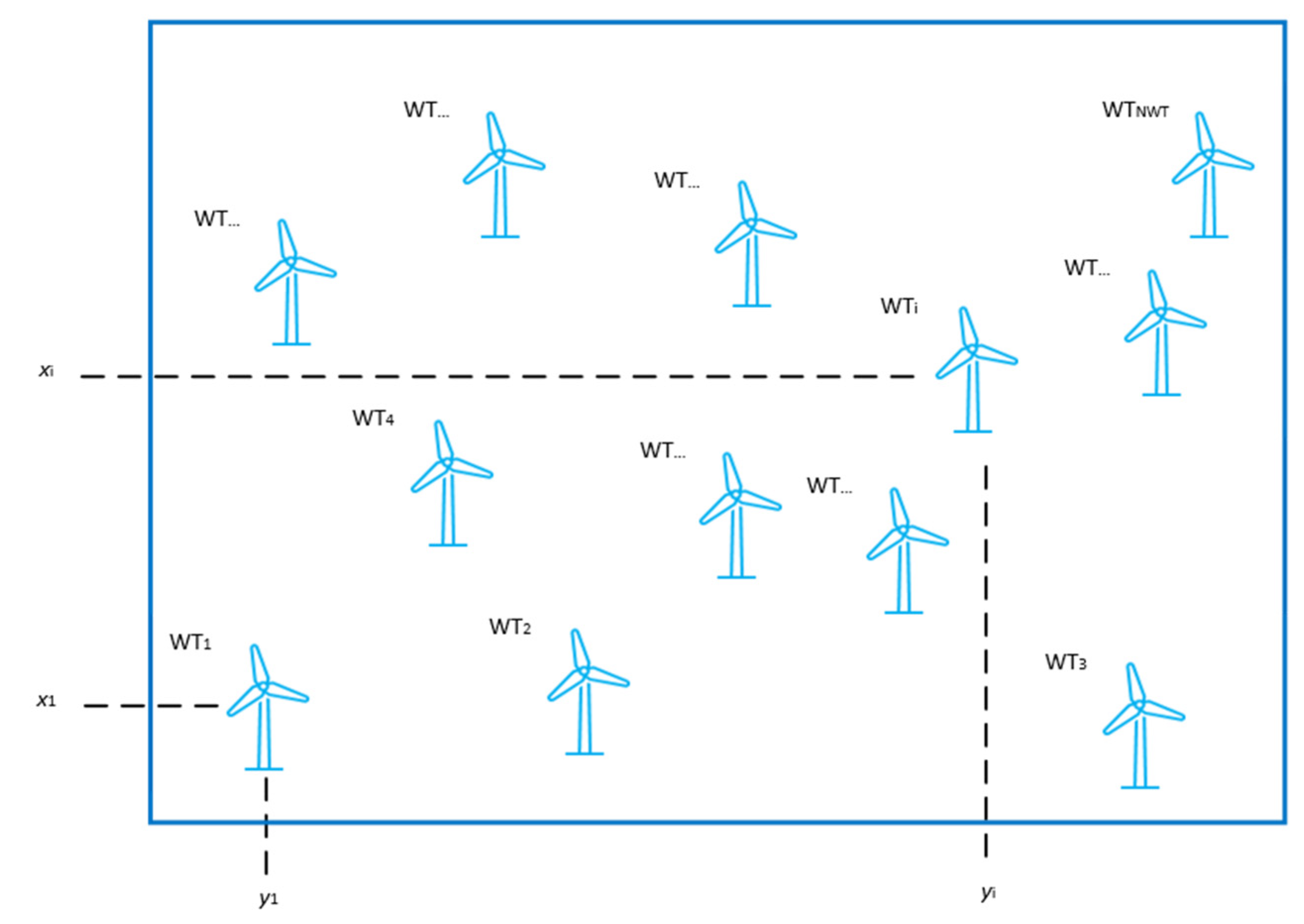
As aforesaid, in this paper, the WFLO/E problem is treated here. The classical WFLO problem consists of finding the optimal locations of WTs inside a given region to optimize certain objective functions (Figure 1). It can be mathematically formulated as follows [60]:

$$\underset{\mathrm{x}\in \mathrm{X}}{\min } F\left(x\right)$$

(1)

where $F$ is the vector of objective functions.

Since two objective functions are used in this work $F$ can be defined by [60]:

$$F\left(x\right)=\left\{f_1\left(x\right),f_2\left(x\right)\right\}$$

(2)

where $x$ is the vector of design variables defined by [60]:

$$x=\left\{x_1,y_1,x_2,y_2,\dots ,x_{\mathrm{NWT}},y_{\mathrm{NWT}},\mathrm{NWT}\right\}\hspace{1em}\hspace{1em}x\in \mathrm{X}$$

(3)

where $x_i$ and $y_i$ are the coordinates of the ${\mathrm{WT}}_i$, $\mathrm{NWT}$ is the number of WTs inside the farm and $\mathrm{X}$ is the feasible set of design variables.

Since the NWT is variable while optimizing the problem, the number of design variables varies, making the problem very difficult to tackle.

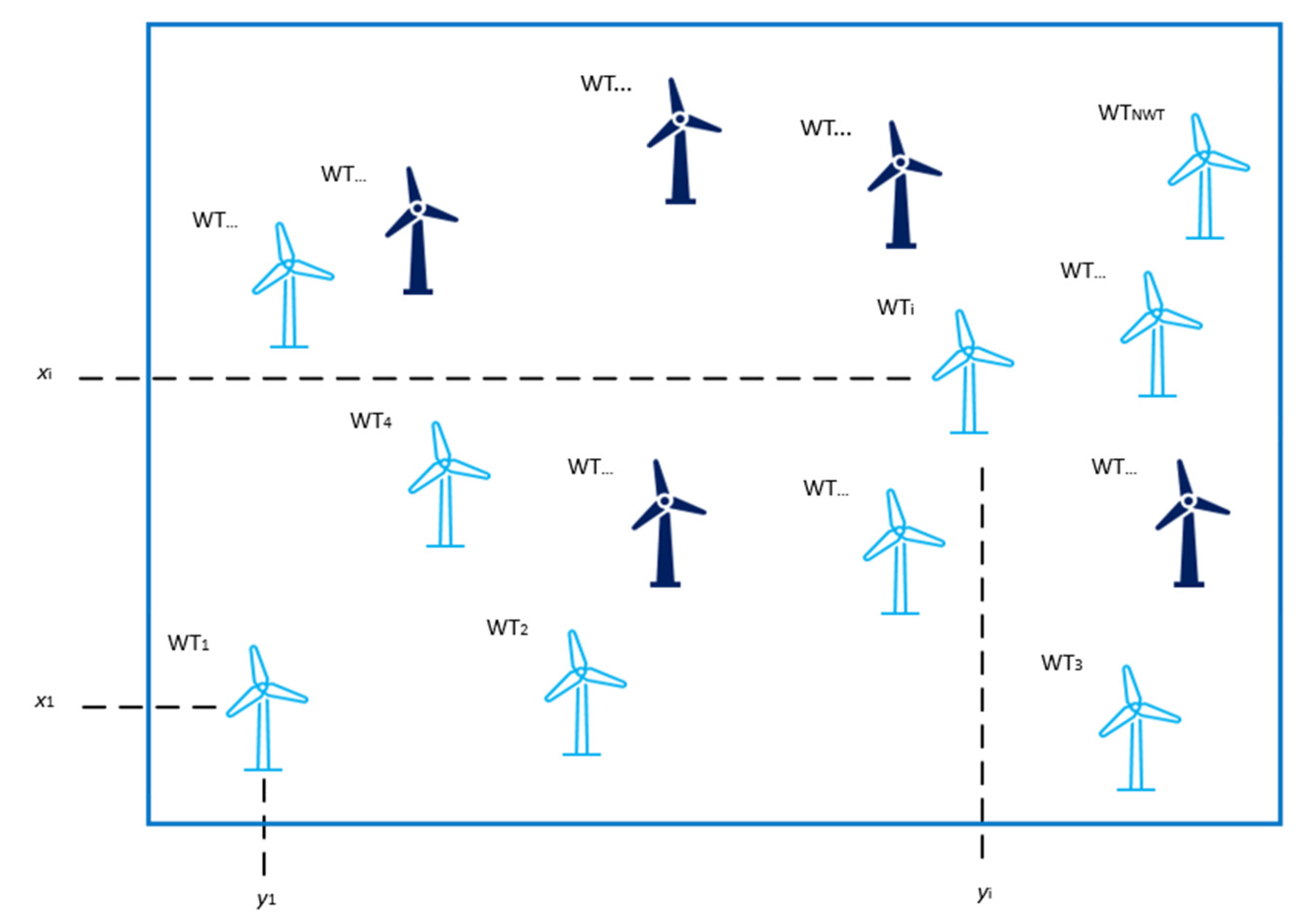
The expansion problem (i.e., the WFLE problem) starts from a wind farm with a given layout (where some WTs are already placed, as seen in Figure 2 with the WTs colored in dark blue). Then, it finds the optimal locations of new WTs (i.e., expanding the existing farm by placing new WTs as seen in Figure 2 with the WTs colored in light blue) to optimize some objective functions. Mathematically, the WFLE problem is formulated as the WFLO problem using Equation (1), where the existing WTs are imposed as additional constraints.

Among the most important factors to consider while optimizing the locations of WTs inside a given region is the wake effect. Therefore, in this section, we first describe the wake model used in this study. Then, the objective functions treated in this paper will be defined.

2.1. Wake Model

When wind passes through a WT, wake flow is produced due to the WT’s wind energy extraction and the rotor’s disturbance. Since WT output power is proportional to the cube of wind speed, wake effects significantly reduce the power and must be taken care of while optimizing the WT layout. The Jensen linear wake decay model [36,37] is utilized to solve the WT wake flow. This wake model assumes [61] the following:

• The wake maintains momentum,
• The wake grows linearly,
• The downstream distance has a linear relationship with the wake’s radius,
• Wakes near the rotor are neglected,
• Absence of rotational flow in the wake, and
• The wake obscures the downstream rotor.

When one WT at the i^th location, as shown in the literature [62], influences the j^th WT, then the following equation can be used to calculate the downstream WT’s wind velocity in the wake region:

$$u_j=u_{0j}\left[1-2d\left(\frac{1}{{\left(1+{\delta }_{i }\frac{x_{ik}}{r_{i1}}\right)}^2}\right)\right]$$

(4)

where ${\delta }_i$ is the entrainment constant, $d$ denotes the axial induction factor, $u_j$ is the wind speed measured at the j^th WT located downstream, u_0j represents the wind speed at the j^th WT, ignoring the effect of the wake created by the previous WTs. The distance between the i^th and j^th WTs is denoted by $x_{ij}$, $r_{i1}$ denotes the downstream rotor radius of the i^th WT. The following expression describes the relationship between the rotor radius of the i^th WT ($r_i$) and the downstream rotor radius of the WT $\left(r_{i1}\right)$ [63]:

$$r_{i1}=r_i{\left(\frac{1-d}{1-2d}\right)}^{\frac{1}{2}}$$

(5)

The following equation is used to obtain the axial induction factor (d) from the WT thrust coefficient (T_C) [63]:

$$d=\frac{1-{\left(1-T_C\right)}^{\frac{1}{2}}}{2}$$

(6)

The following empirical formula may be used to estimate the value of ${\delta }_i$ which is subject to variation depending on the local weather and topography [32].

$${\delta }_i=\frac{1}{2In\frac{h_i}{g_o}}$$

(7)

where $g_0$ denotes the terrain roughness, and h_i is WT hub height.

The wake radius may be calculated using the linear wake model’s conical wake area [63,64]:

$$r_{gi}=r_{i1}+{\delta }_i{x}_{ij}$$

(8)

The logarithmic law is used to extrapolate the wind speed at the j^th WT’s hub height based on the wind speed at a reference height [64,65].

$$u_{0j}=u_R\frac{\ln \frac{h_f}{z_0}}{\ln \frac{h_R}{z_0}}$$

(9)

where $h_f$ is the j^th WT’s hub height, u_R is the wind speed at the reference height and $h_R$ is the reference height.

The given equation only analyzes the wake of one WT. WTs in a wind farm experience several wakes, which increases velocity deficits. Several approaches may be used to represent the stacked impact of several wakes, as mentioned in [66]. In this study, the sum of squares method is employed, as was done in the literature [12,66,67,68]. If many wakes influence the WT, the mixed wake’s kinetic energy deficit is the total of the individual deficits. Hence, the wind speed at the k^th WT is given as:

$$u_k=u_{0k}\left[1-{\left({\displaystyle \sum }_{t=1}^{NWT}{\left(1-\frac{u_{kt}}{u_{0t}}\right)}^2\right)}^{\frac{1}{2}}\right]$$

(10)

where $u_{kt}$ represents the wind velocity at WT $k$ while accounting for the m^th WT’s wake effect, $NWT$ represents the number of WTs, $u_{0k}$ represents the wind velocity at WT k without accounting for the wake effect, and u_0t represents the wind velocity at WT m without accounting for the wake effect.

2.2. Multi-Objective Formulation

The optimization of the windfarm’s efficiency $\eta$ and total power output $P_{Tt}$ is shown in Equation (11) [26]. U_k and u_0k indicate the wind speed with and without upstream WT wakes, respectively. P_k is the k^th WT’s electrical power output against u_k. P_k,max is the k^th WT’s maximum electrical power output against u_0k. $NWT$ is the number of WTs, and f_i is the probability of each wind direction and ${{\displaystyle \sum }}_{i=0}^{360}{f}_j=1$.

$$F=\left\{\begin{array}{c}\eta =\underbrace{\frac{{{\displaystyle \sum }}_{j=0}^{360}{{\displaystyle \sum }}_{k=1}^{NWT}{f}_j P_k\left(u_k\right)}{{{\displaystyle \sum }}_{j=0}^{360}{{\displaystyle \sum }}_{k=1}^{NWT}{f}_j P_{k,max}\left(u_{0k}\right)}}\\ P_{Tt}={\displaystyle {\displaystyle \sum }_{j=0}^{360}}{\displaystyle {\displaystyle \sum }_{k=1}^{NWT}}{f}_j P_k\left(u_k\right)\end{array}\right.$$

(11)

Observing the model’s objectives, the windfarm’s power production rises as the number of WTs increases. Wake flow reduces the windfarm’s efficiency as more WTs are added. Therefore, reducing the number of WTs decreases the wake flow losses and wind farm production. Hence, choosing the best layout and/or expanding the existing layout requires serious consideration and needs to be selected optimally.

2.3. Variable Reduction Approach

In line with our earlier discussion, the WFLO/E problem has been formulated as a multi-objective optimization problem with efficiency and total power as the objectives of interest. Two types of design variables have also been defined, which are the $NWT$, and the location coordinates ($x_i$ and $y_i$) of WTs. Therefore, the total number of design variables is $2\times NWT$. Hence, for a modest number of WTs, the number of design variables is double that, which could be a significant number for most optimization algorithms. This complexity of the WFLO/E problem is buttressed by the variability of the number of design variables due to changing $NWT$.

This paper proposes two approaches for simplifying the WFLO/E problem. The first approach creates a grid spanning the wind farm’s geographical area. The cells in the grid represent the WT locations (a WT can be located at the center of the cell) and their number is equal to the maximum number of WTs placed in the site. A binary representation can then be employed such that a cell with a WT inside it is marked with a “1” and a cell without a WT inside it is marked with a “0”. This approach offers two main advantages: it solves the problem of the variability of the number of design variables and halves the number of design variables. Rather than determining coordinates $x_i$ and $y_i$, only cell locations are determined based on a binary variable.

The second approach, which further reduces the number of design variables, is as follows. A column of cells is considered one binary number, with the number of bits equal to the number of rows.

To illustrate this, let us take the example of a wind farm shown in Figure 3. On this farm, there is a grid of 20 $\left(4\times 5\right)$ cells (i.e., the maximum NWT = 20). It can be seen from this figure that there are 9 WT placed inside the farm (i.e., NWT = 9). The first column corresponds to the binary digits 1, 0, 0 and 1, equivalent to the binary number 1001 or decimal number 9. This value represents the placement of two WTs, one in each of the first and fourth cells of the column. Similarly, since there are WTs placed in the first, third and fourth cells of column 2, the equivalent binary number is 1011 (or decimal number 11). This representation reduces the number of design variables in the problem represented in Figure 3 from 20 to 5. Generally, the approach will reduce the number of design variables from the number of cells to the number of columns. Hence, there is an N-fold reduction for a typical $\left(N\times M\right)$ grid.

The synergetic adoption of the two approaches considerably reduces the number of design variables, simplifying the optimization problem.

3. The Multi-Objective Evolutionary Algorithm Based on an Enhanced Inverted Generational Distance Metric Combined with the Two-Archive Algorithm 2 (MOEA/IGD-NS/TA2)

The proposed approach combines EA-based Enhanced Inverted Generational Distance Metric (MOEA/IGD-NS) and EA-based Two-Archive Algorithm 2 (Two Arch2). Therefore, in the following sections, we will first describe the two combined algorithms separately and then describe the combined approach to present the proposed MOEA/IGD-NS/TA2 approach.

3.1. The Multi-Objective Evolutionary Algorithm Based on an Enhanced Inverted Generational Distance Metric (MOEA/IGD-NS)

Among the essential components of MOEAs, environmental selection plays a vital role in determining the generational survival of candidate solutions. Over time, performance metrics have proven to be valuable tools for environmental selection [55,57,69]. One such metric is the inverted generational distance (IGD) [70]. MOEA/IGD-NS uses IGD, defined in Equation (12), with non-contributing solution deletion (NS) to evaluate the quality of solutions in diversity and convergence. It discriminates against non-contributing solutions from each non-dominated front. Candidate solutions with minimal contributions are removed until the desired population size is attained.

$$IGD\left(P,P^{*}\right)=\frac{{{\displaystyle \sum }}_{x\in P^{*}}\underset{y\in P}{\min } dis\left(x,y\right)}{\left|P^{*}\right|}$$

(12)

where $P$ represents the objective values of a set of non-dominated solutions from any MOEA, $P^{*}$ is the set of uniformly distributed reference points sampled from the Pareto Front (PF), and $dis\left(x,y\right)$ is the Euclidean distance between points $x$ and $y$. IGD computes the average minimum distance from each point in $P^{*}$ to those in $P$. The implication is that it measures both the convergence and diversity of the solution set $P.$ Therefore, smaller IGD values imply better diversity and convergences such that an $IGD\left(P,P^{*}\right)$ of zero implies that $P^{*}$ is a subset of $P$. Similar to $IGD$ is the generational distance (GD) defined in Equation (13), which computes the average minimum distance from each point in $P$ to the points in $P^{*}$ [71]. A smaller value of GD also implies better convergence, but GD cannot evaluate the diversity of $P$.

$$GD\left(P,P^{*}\right)=\frac{\sqrt{{{\displaystyle \sum }}_{y\in P}\underset{x\in P^{*}}{\min } dis{\left(x,y\right)}^2}}{\left|P\right|}$$

(13)

The parameter ${\mathsf{\Delta }}_p, p>1$ is another performance metric based on IGD and GD defined in Equation (14) [72]. It can determine non-contributing solutions and evaluate the diversity and convergence of the solution set.

$${\mathsf{\Delta }}_p\left(P,P^{*}\right)=\max \left(G{D}_p\left(P,P^{*}\right),IG{D}_p\left(P,P^{*}\right)\right)$$

(14)

where

$$G{D}_p\left(P,P^{*}\right)={\left(\frac{1}{\left|P\right|}{{\displaystyle \sum }}_{y\in P}\underset{x\in P^{*}}{\min } dis{\left(x,y\right)}^p\right)}^{1/p}$$

$$IG{D}_p\left(P,P^{*}\right)={\left(\frac{1}{\left|P^{*}\right|}{{\displaystyle \sum }}_{x\in P^{*}}\underset{y\in P}{\min } dis{\left(x,y\right)}^p\right)}^{1/p}$$

The solutions ignored in IGD calculation due to non-neighborhood to any reference point are termed non-contributing solutions in a non-dominated solution set. More formally, the solution $y^{\prime }$ is a non-contributing solution in a non-dominated solution set $P$ for a given $P^{*}$ if it satisfies the condition:

$$\nexists x\in P^{*}:dis\left(x,y^{\prime }\right)=\underset{y\in P}{\min } dis\left(x,y\right)$$

(15)

Therefore, the IGD with non-contributing solution detection (IGD-NS) is defined as:

$$IGD-NS\left(P,P^{*}\right)={{\displaystyle \sum }}_{x\in P^{*}}\underset{y\in P}{\min } dis\left(x,y\right)+{{\displaystyle \sum }}_{y^{\prime }\in P^{\prime }}\underset{x\in P^{*}}{\min } dis\left(x,y^{\prime }\right)$$

(16)

where $P^{\prime }$ is the set of non-contributing solutions in population $P$. Therefore, a good (small) value of IGD-NS, can be obtained if and only if the population has good convergence, good diversity and contains the fewest non-contributing solutions possible.

MOEA/IGD-NS iteratively eliminates candidate solutions with the most negligible contribution to the IGD-NS metric until a predefined population size is attained. The framework is itemized in Algorithm 1 and begins with a random population $P$ with $N$ individuals. $P$ is used to update an external archive using the procedure itemized in Algorithm 2. The archive is updated by first copying all the non-dominated solutions in $P$ to $NDS$. The archive $A$ is then filled with the extreme solutions of $NDS,$ and if the size of $A$ is greater than the required archive size $NA,$ ($NA-\left|A\right|)$ solutions are randomly eliminated. Alternatively, $A$ is filled by solution $p$ one by one until $\left|A\right|=NA$. After which, the evolutionary process continues iteratively until the termination condition is achieved. In doing this, $N$ offsprings are generated and added to the parent population, and the archive is updated with $A\cup P$ as outlined in Algorithms 1 and 2. Finally, the environmental selection is performed as outlined in Algorithm 3.

Algorithm 1: General Framework of MOEA/IGD-NS
	Input: $\mathrm{Population} \mathrm{size}, N,$$\mathrm{Archive} \mathrm{size} NA$
	Output: Final population, $P$
	1	Initialization: Randomly initialize population $P$ of size $N$.
	2	Update Archive using $P$$\mathrm{and} NA$ (UpdateArchive (P, NA))
	3	$\mathrm{Determine} \mathrm{solutions} \mathrm{with} \mathrm{maximal} \mathrm{or} \mathrm{minimal} \mathrm{objective} \mathrm{values} \mathrm{in} A_D^{*}$$\mathrm{and} \mathrm{move} \mathrm{them} \mathrm{to} A_D$;
	4	while termination criteria is not fulfilled do
	5		$\mathrm{Carryout} \mathrm{variation} \mathrm{operation} \mathrm{on} \mathrm{population}, P=P \cup \mathrm{variation}\left(P,N\right)$;
	6		$\mathrm{Update} \mathrm{the} \mathrm{archive}, A=\mathrm{UpdateArchive}\left(A\cup P,NA\right)$;
	7		$\mathrm{Carryout} \mathrm{environmental} \mathrm{Selection}, P=\mathrm{EnvironmentalSelection}\left(P, A, N\right))$;
	8	end
	9	$\mathrm{Output} P.$

Algorithm 2: UpdateArchive (P, NA)
	Input: $\mathrm{Current} \mathrm{Population}, P,$$\mathrm{Archive} \mathrm{size} NA$
	Output: New Archive, $A$
	1	Obtain the non-dominated solutions in $P,NDS=\mathrm{NondominatedSolution}\left(P\right)$
	2	$\mathrm{Update} \mathrm{the} \mathrm{Archive} \mathrm{with} \mathrm{extreme} \mathrm{solutions} \mathrm{in} \mathrm{NDS} A=ExtremeSolution\left(NDS\right)$
	3	if$\left|A\right|>NA$do
	4		$\mathrm{Randomly} \mathrm{delete} \left|A\right|$–NA solutions from $A$
	5	else
	6		while$\left|A\right|<NA and \left|A\right|<\left|NDS\right|$do
	7			$P=argma{x}_{p\in NDS\backslash A}mi{n}_{q\in A}arccosine\left(p,q\right)$;
	8			$A=A\cup \left\{p\right\}$;
	9		end while
	10	end if
	11	Output A.

The environmental selection is initiated with non-dominated sorting. This sorting involves dividing the combined population $P$ into non-dominated fronts $F_1,F_2 \dots$ using efficient non-dominated sorting (ENS) [73]. This is followed by the selection of the first $k$ fronts. The variable $k$ is the maximum value satisfying the condition $\left|F_1\cup F_2\cup \dots \cup F_k\right|<N$. In the next step, solutions in $F_{k+1}$ are eliminated iteratively until the condition $\left|F_{k+1}\right|<N-\left|P\right|$ is met. The solution eliminated each time, $y^{\prime }$ is such that:

$$y^{\prime }=argmi{n}_{y\in F_{k+1}}IGD-NS\left(F_{k+1}\backslash \left\{y\right\},A\right)$$

(17)

The algorithm is concluded by adding the remaining solutions in $\left|F_{k+1}\right|$ to $P$.

Algorithm 3: EnvironmentalSelection (P, A, N)
	Input: $\mathrm{Combined} \mathrm{Population}, P,$ Archive, $A$, population size, $N$
	Output: population for next generation, $P$
	1	$F=\mathrm{NondominatedSort}\left(P\right)$;
	2	$\mathrm{Find} P=F_1\cup F_2, \dots F_k, k is the maximal value sch that \left|F_1\cup F_2, \dots F_k\right|<N$
	3	while$\left|F_k\right|>N-\left|P\right|$do
	4		$\mathrm{Find} y^{\prime }$$\mathrm{in} F_{k+1}$ using Equation (15);
	5		$F_{k+1}=F_{k+1}\backslash \left\{y^{\prime }\right\}$;
	6	end while
	7	$P=P\cup F_{k+1};$
	8	Output P.

3.2. Two-Archive Algorithm 2 (Two_Arch2)

The improved two-archive algorithm (Two_Arch2) was proposed in [59] to balance the performance of MaOEAs in three metrics of convergence, diversity and complexity. Hence, it is a low-complexity EA with two archives, the convergence archive (CA) and diversity archive (DA), that treat convergence and diversity independently using an indicator and Pareto-based principles, respectively. It uses an $L_p$-norm-based diversity maintenance scheme. The concept of Two_Arch2 was developed from Two_Arch [74]. The flowchart for the two algorithms is presented in Figure 4a,b for comparison purposes.

The Two_Arch2 algorithm is designed to have a crossover operation between CA and DA, where mutation occurs in CA only during reproduction. Therefore, CA has impoverished diversity, and only DA is used as the final output of the algorithm. The quality indicator, $I_{\epsilon +}$ is used for selection in the CA phase which quantifies the minimum distance requirement for a solution to dominate in the objective space [69]. The fitness $F\left(x_1\right)$, which is a measure of $I_{\epsilon +}$ when an individual $x_1$ is deleted from the population is as given by Equation (19).

$$I_{\epsilon +}\left(x_1,x_2\right)=\underset{\epsilon }{\min }(f_i(x_1-\epsilon \le f_i\left(x_2\right),1\le i\le m$$

(18)

$$F\left(x_1\right)={{\displaystyle \sum }}_{x_2\in P\left\{x_1\right\}}-e^{-I_{\epsilon +}\left(x_1,x_2\right)/0.05}$$

(19)

The first step in updating CA is the addition of offspring, and then extra solutions are deleted using the fitness by removing solutions with the smallest $I_{\epsilon +}$. Finally, the $I_{\epsilon +}$ of the remaining individuals in the population are updated according to Algorithm 4. This update will generate a CA with a fixed number of solutions.

Algorithm 4: Selection in an Overflowed CA.
	Input: $A_C$$-\mathrm{the} \mathrm{overflowed} \mathrm{CA}, n_{CA}$$-\mathrm{the} \mathrm{fixed} \mathrm{size} \mathrm{of} A_C$
	Output$: \mathrm{updated} A_C$-CA
	1	While $\left|AC\right|>n_{CA}$do
	2		$\mathrm{Find} \mathrm{the} \mathrm{individual} x^{*}$$\mathrm{with} \mathrm{the} \mathrm{minimal} F{x}^{*}$
	3		$\mathrm{Delete} x^{*}$$\mathrm{from} A_C$
	4		$\mathrm{Update} \mathrm{the} \mathrm{population} \mathrm{using} F\left(x\right)=F\left(x\right)+e^{-I_{\epsilon +}\left(x_1,x_2\right)/0.05}$
	5	end
	6	$\mathrm{Output} A_C$.

Maintaining the diversity of MaOPs, a challenging task, can be achieved easily in two ways. The first is by distributing solutions in the entire high-dimensional objective space to capture the maximum information on the PF. The second approach maximizes solutions’ differences when projected to a low-dimensional objective space. Two_Arch2 uses Pareto dominance to update the DA with non-dominated solutions, and the concept of selection is used to keep required individuals when the DA overflows. The algorithm for selection in an overflowed DA is itemized in Algorithm 5. The solutions with maximal or minimal objectives (boundary solutions) are selected first and then using $L_p$-norm as a similarity measure, the solutions with the most significant difference from the initially selected solutions are chosen iteratively. The parameter $p$ (in the $L_p$-norm) is selected to be less than one because previous studies have shown that smaller values of $p$ ensure higher contrast between closest and furthest neighbors [75]. Specifically, for $m$ number of objectives, the value $p=1/m$ is used as proposed in [59].

Algorithm 5: Selection in an Overflowed DA
	Input: $A_D^{*}$$-\mathrm{the} \mathrm{overflowed} \mathrm{DA}, n_{DA}$$-\mathrm{the} \mathrm{fixed} \mathrm{size} \mathrm{of} \mathrm{AD}, A_C$
	Output: $A_D$
	1	$\mathrm{Set} A_D$ empty;
	2	$\mathrm{Determine} \mathrm{solutions} \mathrm{with} \mathrm{maximal} \mathrm{or} \mathrm{minimal} \mathrm{objective} \mathrm{values} \mathrm{in} A_D^{*}$$\mathrm{and} \mathrm{move} \mathrm{them} \mathrm{to} A_D$;
	3	While$A_D$ is not full do
	4		for$\mathrm{each} \mathrm{member} i$$\mathrm{in} A_D^{*}$do
	5			$\mathrm{Similarity}[i]=\min \left(\mathrm{distance}\left(i,j\right)\right), j\in A_D$
	6		end
	7		$I=argmax\left(Similarity\right)$, move solution $I$$\mathrm{from} A_D^{*}$$\mathrm{to} A_D$
	8	end
	9	$\mathrm{Output} A_D$.

3.3. The Proposed MOEA/IGD-NS/TA2 Approach

The general framework of the proposed MOEA/IGD-NS/TA2 is given in Algorithm 6. As aforesaid, it combines the two EA-based approaches described in the Section 3.1 and Section 3.2. In this approach, first, a population of $N$ size is randomly generated inside the search space. This population is used then to update three archives called $A$, $CA$ and $DA$ as it can be shown in Algorithm 6 (from lines 4 to 6). The $A$, $CA$ and $DA$ archives have the predefined $NA$, $C{A}_{size}$ and $D{A}_{size}$ sizes, respectively. After that, the MOEA/IGD-NS/TA2 iterates until a termination criterion is met. In these iterations, the population’s quality is improved using the following steps. First, offsprings $\left(O_1\right)$ are obtained using the variation process (Algorithm 6 line 5). Second, other offsprings $\left(O_2\right)$ are obtained by carrying out a variation operation process between the population $\left(P\right)$ and the $CA$ and $DA$ archives (Algorithm 6 line 9). In the next three steps (shown in lines 10 to 12 in Algorithm 6), the archives $A$, $CA$ and $DA$ get updated using the previous archives and the new offsprings: $O_1$ and $O_2$. Finally, the last step in the iterative process consists of carrying out an environmental selection between the previous population $P$, the new offspring $O_1\mathrm{and} O_2$, and the archive $A$. The output of the algorithm is the improved and updated population $P$.

Algorithm 6: General Framework of the proposed MOEA/IGD-NS/TA2.
1	Input: $\mathrm{Population} \mathrm{size} \left(N\right)$$, \mathrm{Archive} \mathrm{size} \left(NA\right)$$, \mathrm{Convergence} \mathrm{Archive} \mathrm{size} \left(C{A}_{size}\right)$$, \mathrm{Diversity} \mathrm{Archive} \mathrm{size} \left(D{A}_{size}\right)$
2	Output: $\mathrm{Final} \mathrm{population} \left(P\right)$
3		Initialization: Randomly initialize population $P$ of size $N$.
4		$A=\mathrm{UpdateArchive} \left(P, NA\right)$;
5		$CA=\mathrm{UpdateCA}\left(P,C{A}_{size}\right)$;
6		$DA=\mathrm{UpdateDA}\left(P,D{A}_{size}\right)$;
7		while termination criteria is not fulfilled do
8			$O_1=P\cup \mathrm{Variation}\left(P,N\right)$;
9			$O_2=CA DA\cup \mathrm{Variation}\left(P,N\right)$;
10			$CA=\mathrm{UpdateCA}\left(CA,O_1,O_2,C{A}_{size}\right)$;
11			$DA=\mathrm{UpdateDA}\left(DA,O_1,O_2,D{A}_{size}\right)$;
12			$A=\mathrm{UpdateArchive}\left(A,O_1,O_2,NA\right)$;
13			$P=\mathrm{EnvironmentalSelection}\left(P, O_1,O_2,A, N\right))$;
14		end

3.4. Implementation of the Proposed MOEA/IGD-NS/TA2 Approach to Solve the WFLO/E Problem

The flowchart of the implementation of the proposed approach to solve the WFLO/E problem is given in Figure 4c. The overall process starts by defining the needed data like wind speed the farm location the type of WTs to be used, etc. After that, the type of problem to be solved is identified. In other words, is it a WFLO problem or the WFLE one. Then, the optimization process parameters are defined like the population size, number of iterations and any internal parameter for the MOEA/IGD-NS/TA2. Once all the data and needed parameters are defined the optimization process using the proposed MOEA/IGD-NS/TA2 algorithm is run. This process terminates after certain criteria re met, for example after the maximum number of iterations is exceeded. Finally, the PF is displayed as the final step.

4. Application and Results

4.1. Wind, Wind Farm, and Turbine Data

Layout optimization models often assume constant wind speed and direction while modeling, which is not true in the real sense. Therefore, the use of Midland Texas wind probability distribution for April to predict wind conditions [26] is adopted in this paper to duplicate the practical scenario. Since wakes near the rotor are not incorporated in the Jensen linear wake model and commercial WTs are seldom built close together, the grid size for all case studies in this paper is a 6 km × 2 km rectangle wind farm with 0.3 km × 0.4 km cells. WTs are usually installed in each cell’s middle, giving 100 possible positions. Therefore, the selected grid must satisfy the required safety spacing between the WTs so that one accidental fall will not affect others.

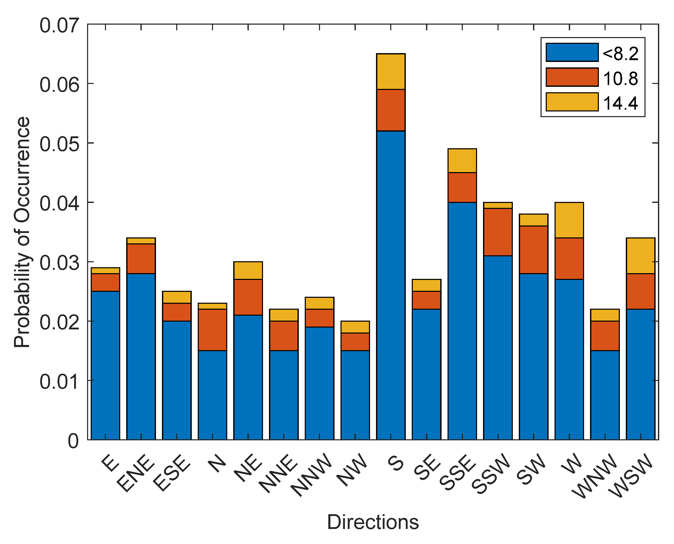
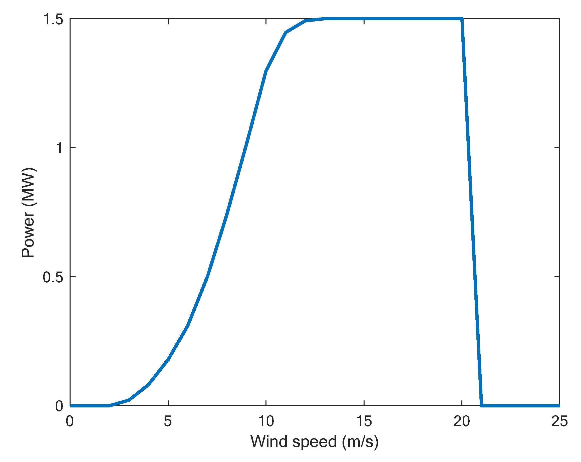
The wind probability distribution diagram for Midland, Texas, is presented in Figure 5. It can be seen from this figure that the wind is dominant from the south direction. More information about locations and wind speed is available at [26]. Furthermore, the real/commercial ‘Acciona AW82/1500 kW’ WT with 60 m hub height is used in this study. The output power as the function of wind speed is represented in Figure 6, whilst

Table 1. Technical characteristics for the WT used in this study.

Model	Acciona AW82/1500 kW
Rated Power (MW)	1.5
IEC Classes	IIIb
Hub Height (m)	60, 80
Rotor Diameter (m)	82
Cut-in speed (m/s)	3
Cut-out speed (m/s)	20

lists all technical characteristics related to this WT.

Furthermore, although the Capacity Factor ($Cf)$ is not considered as n objective function in the optimization process, it has been reported in all cases to indicate how much energy a given wind farm produces in a given site or place. As reported in [26], for a wind farm, the $Cf$ ranges between 20% and 50%.

4.2. Investigated Cases

MATLAB^® was used to simulate all six cases investigated in this paper. A $\left(20\times 5\right)$ grid was created for each case so that each cell of the grid can contain at most a single WT, making the maximum number of WTs 100. Applying the variable reduction technique discussed in Section 3, the design variables are reduced by 90%. The investigated cases are presented and discussed in the following subsections.

4.2.1. CASE 1

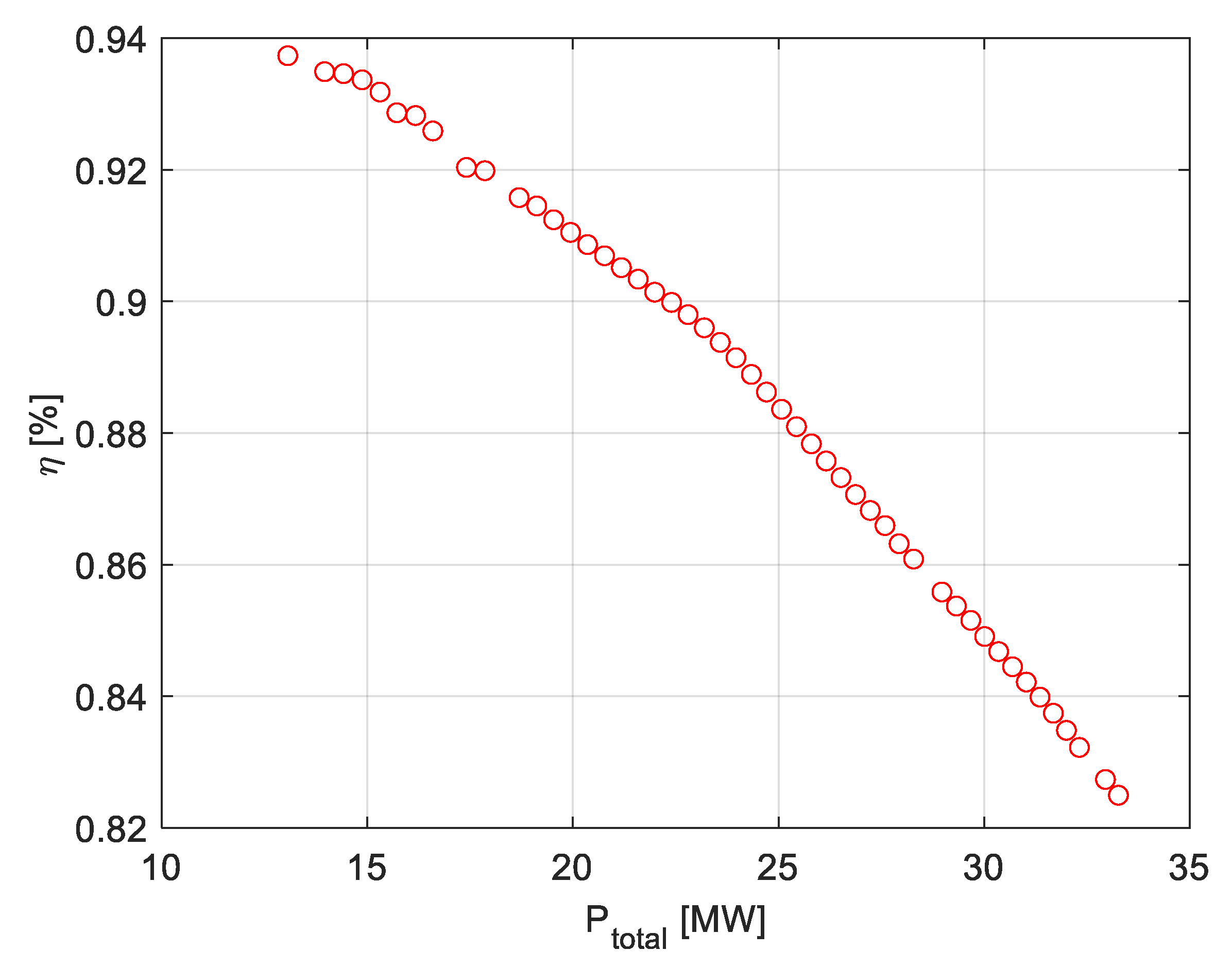
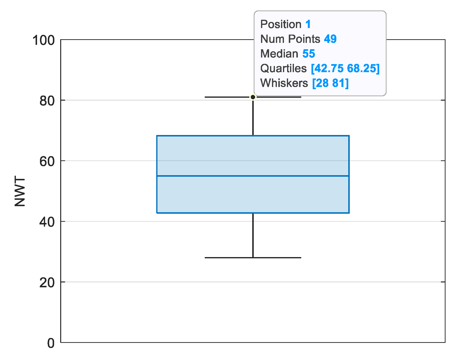
In this case (a WFLO case), the considered farm can have 1 to 100 WTs, and there are no pre-fixed locations of WTs. The proposed MOEA/IGD-NS/TA2 approach has been run for this case, and the obtained set of solutions (i.e., the PF) is represented in Figure 7. This PF is composed of 49 solutions with different NWTs ranging from 28 to 81, as shown in the box plot of Figure 8. It is worth mentioning that, although there were no constraints on the NWT in this case, the solutions found 28 < NWT < 81. In other words, no solutions were found with NWT less than 28 or greater than 81.

It can be seen from Figure 7 that the PF is not entirely smooth. That is due to two factors: (1) the locations of WTs are discrete values, and therefore, with the same number of WTs, we can find a couple of different solutions, and (2) the random nature of wind probabilities.

Nine selected results among the obtained ones where NWT ranges from the smallest value to the highest one are tabulated in

Table 2. Some selected layouts obtained for CASE 1.

Solution #	NWT	${\mathit{P}}_{\mathit{t}\mathit{o}\mathit{t}\mathit{a}\mathit{l}}$ [MW]	$\mathit{\eta }$ [%]	$\mathit{C}\mathit{f}$ [%]
1	28	13.07	93.74	31.11
2	35	16.17	92.83	30.81
3	43	19.53	91.24	30.28
4	49	21.99	90.14	29.92
5	55	24.34	88.89	29.50
6	61	26.52	87.32	28.98
7	68	28.97	85.58	28.40
8	74	31.02	84.21	27.95
9	81	33.26	82.49	27.38

. The following comments can be made from that table:

▪

The selected solutions have 28, 35, 43, 49, 55, 61, 68, 74 and 81WTs, respectively.

▪

The lowest $\eta$ found is 82.49% for $NWT=81$, and the highest $\eta$ is 93.74% for NWT = 34.

▪

The lowest total power obtained is 13.07 MW for NWT = 28, and the highest total power is found to be 33.26 MW for NWT = 81.

▪

The $Cf$ varies between 27.38% and 31.11%, which is acceptable since they fall between 20% and 50%.

The optimal layouts selected for this case are represented in Figure 9. It can be noticed from this figure that when the number of WTs is low, they tend to be located far from each other. This is mainly to reduce the wake effect. It is also evident that wind directions have a significant role in optimizing the locations of WTs.

4.2.2. CASE 2

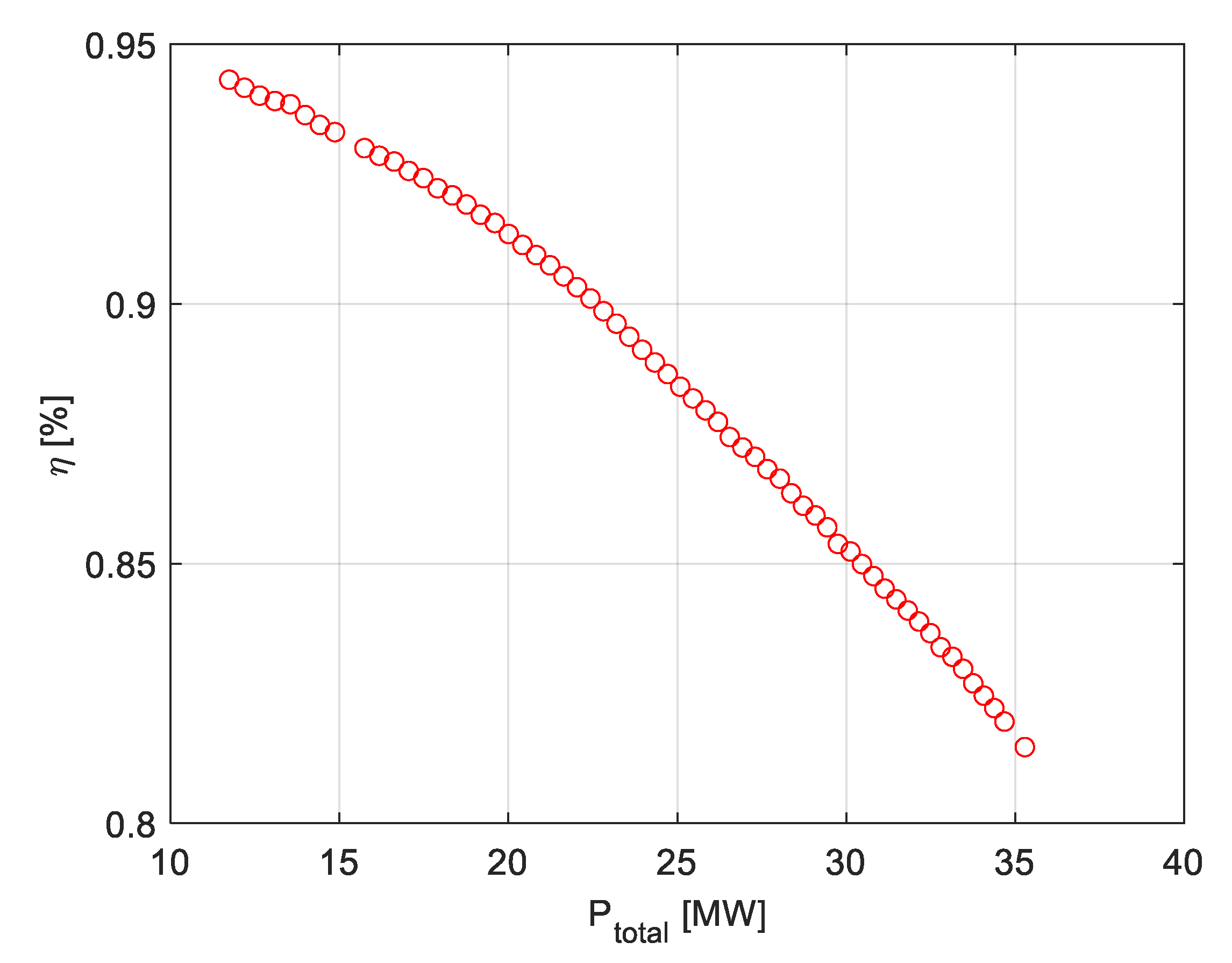
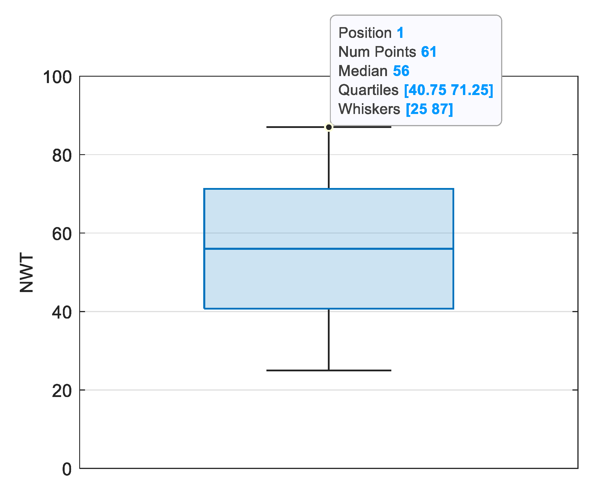
This is an WFLE case where WTs located at locations # 1, 26, 40 and 85 are fixed (the numbering of WTs starts from the lower left corner cell of the grid and goes right and then up till it reaches the upper-right corner cell). The allowed NWT is between 1 and 100, which means there are no constraints imposed on NWT. The proposed MOEA/IGD-NS/TA2 approach has been tried in this case, and the obtained PF is represented in Figure 10. This PF is composed of 61 solutions with different NWTs ranging from 25 to 87, as shown in the box plot of Figure 11.

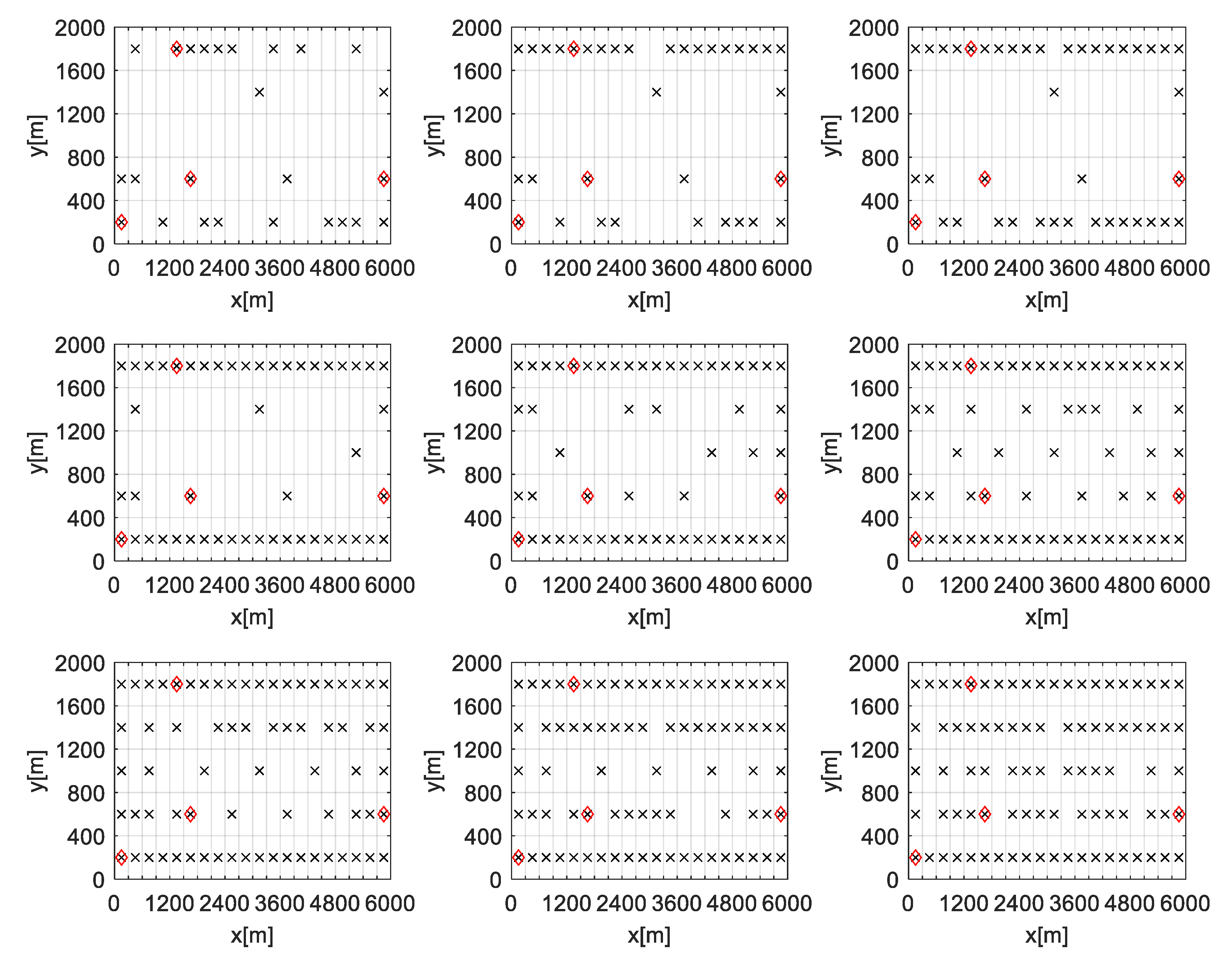
Nine selected results among the obtained ones, where NWT ranges from the least value to the highest one, are tabulated in

Table 3. Some selected layouts obtained for CASE 2.

Solution #	NWT	${\mathit{P}}_{\mathit{t}\mathit{o}\mathit{t}\mathit{a}\mathit{l}}$ [MW]	$\mathit{\eta }$ [%]	$\mathit{C}\mathit{f}$ [%]
1	25	11.74	94.32	31.30
2	34	15.74	93.00	30.86
3	41	18.76	91.92	30.50
4	49	22.03	90.32	29.98
5	56	24.71	88.65	29.42
6	64	27.66	86.82	28.81
7	71	30.13	85.23	28.29
8	79	32.79	83.39	27.67
9	87	35.28	81.47	27.04

, and their corresponding optimal layouts are represented in Figure 12. The following comments can be made:

▪

The selected solutions have 25, 34, 41, 49, 56, 64, 71, 79 and 87 WTs, respectively.

▪

The first layout obtained with NWT = 25 has the highest $\eta$ (94.32%) and the lowest $P_{total}$ (11.74 MW).

▪

The last layout obtained with NWT = 87 has the lowest $\eta$ (81.47%) and the highest $P_{total}$ (35.28 MW).

▪

The $Cf$ varies between 27.04% and 31.30%, which is acceptable since they fall between 20% and 50%.

▪

In all the obtained solutions, WTs are found to be located at the imposed locations (i.e., at locations # 1, 26, 40 and 85), represented by a red diamond in Figure 12.

4.2.3. CASE 3

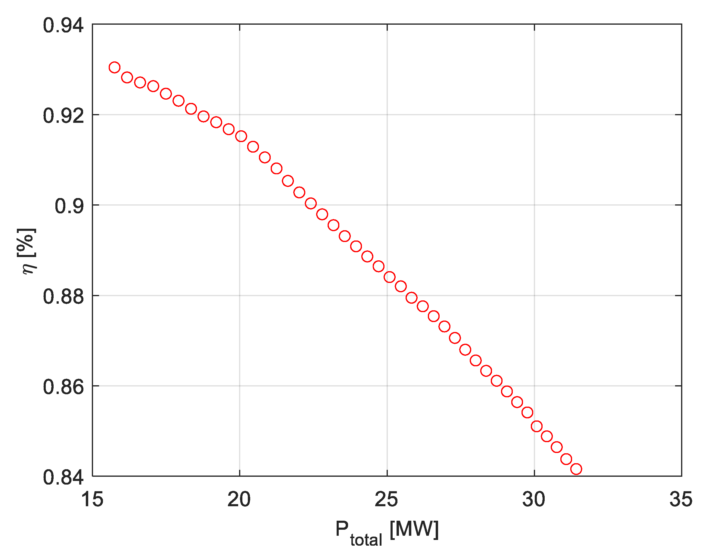
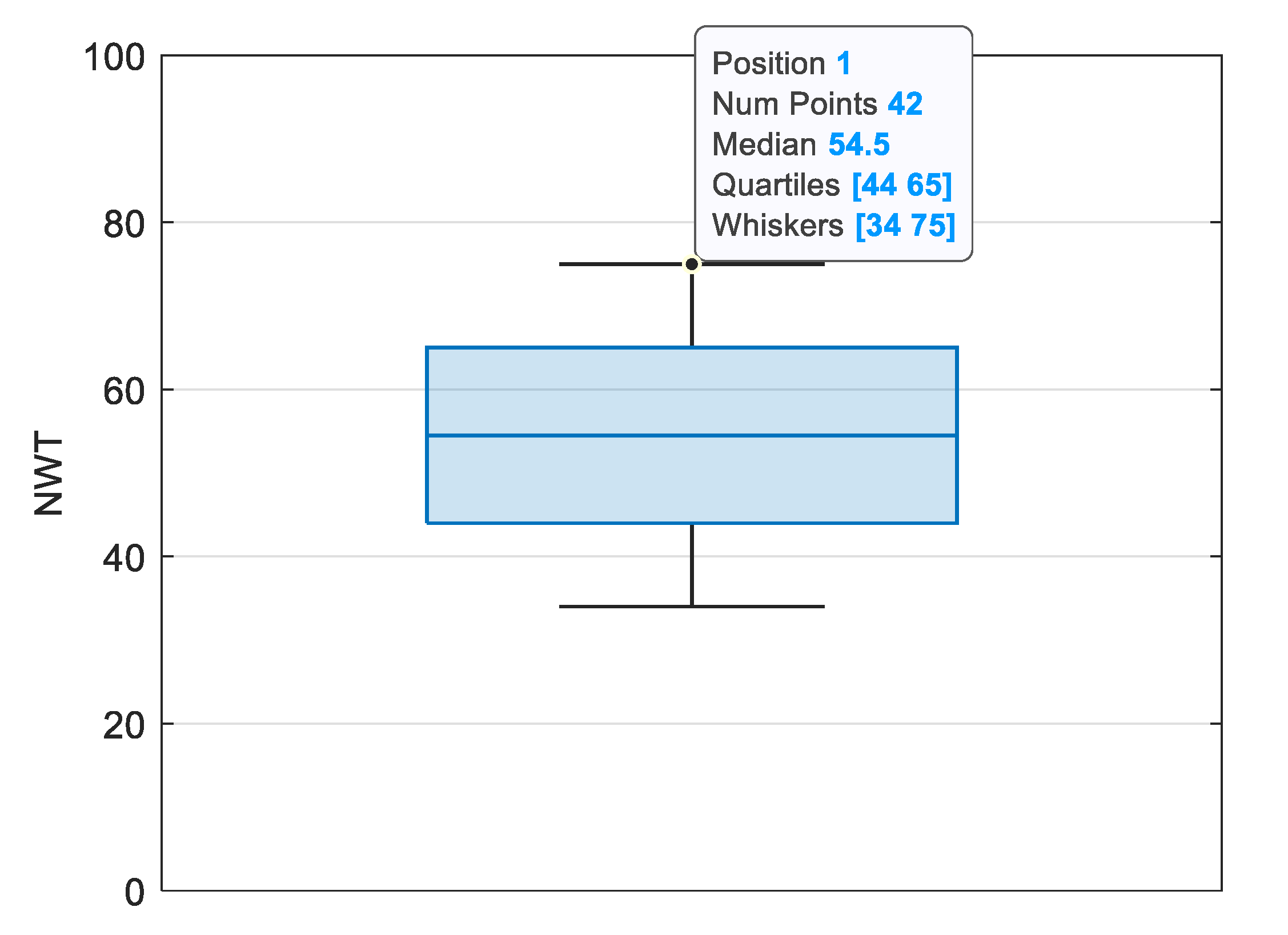
This is a WFLE case where WTs located at locations # 1, 26, 40 and 85 are fixed. An additional constraint is imposed on the allowed NWT per layout (25 < NWT < 75). The proposed MOEA/IGD-NS/TA2 approach has been run for this case, and the obtained PF is represented in Figure 13. This PF is composed of 42 solutions with different NWT ranging from 34 to 75, as shown in the box plot of Figure 14.

Nine selected results among the obtained ones where NWT ranges between the least value (i.e., NWT = 34) and the highest (i.e., NWT = 75) are tabulated in

Table 4. Some selected layouts obtained for CASE 3.

Solution #	NWT	${\mathit{P}}_{\mathit{t}\mathit{o}\mathit{t}\mathit{a}\mathit{l}}$ [MW]	$\mathit{\eta }$ [%]	$\mathit{C}\mathit{f}$ [%]
1	34	15.75	93.04	30.88
2	39	17.92	92.31	30.63
3	44	20.05	91.52	30.37
4	49	22.02	90.28	29.96
5	55	24.33	88.86	29.49
6	60	26.21	87.76	29.13
7	65	28.01	86.56	28.73
8	70	29.76	85.41	28.35
9	75	31.42	84.16	27.93

, and their corresponding optimal layouts are represented in Figure 15. The following comments can be made from Table 4 and Figure 15:

▪

The nine selected solutions have NWT values: of 34, 39, 44, 49, 55, 60, 65, 70 and 75, respectively.

▪

The layout with the least value of NWT (25) has the lowest $P_{total}$ (15.75 MW) and the highest $\eta$ (93.04%).

▪

The layout with the largest value of NWT (75) has the lowest $\eta$ (84.16%) and the highest $P_{total}$ (31.42 MW).

▪

The $Cf$ varies between 27.93% and 30.88%, which falls between the acceptable range of 20% and 50%.

▪

In all the obtained solutions, WTs were located at the imposed locations (i.e., locations # 1, 26, 40 and 85), represented by the red-shaped diamond in Figure 15.

▪

The obtained values of NWT are between 25 and 75 as imposed by the designer/planner.

4.2.4. CASE 4

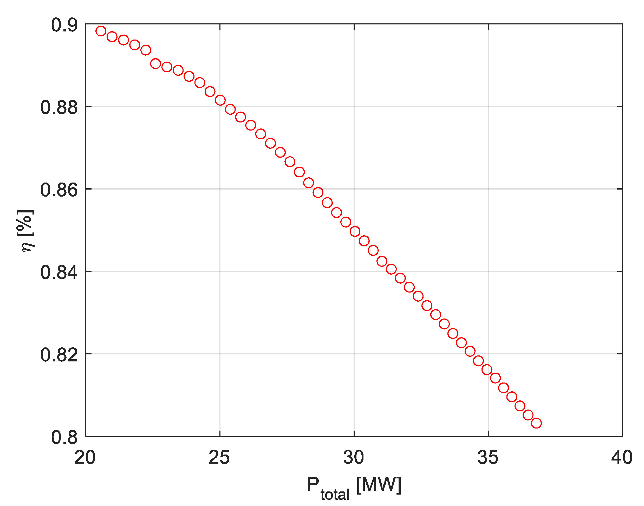
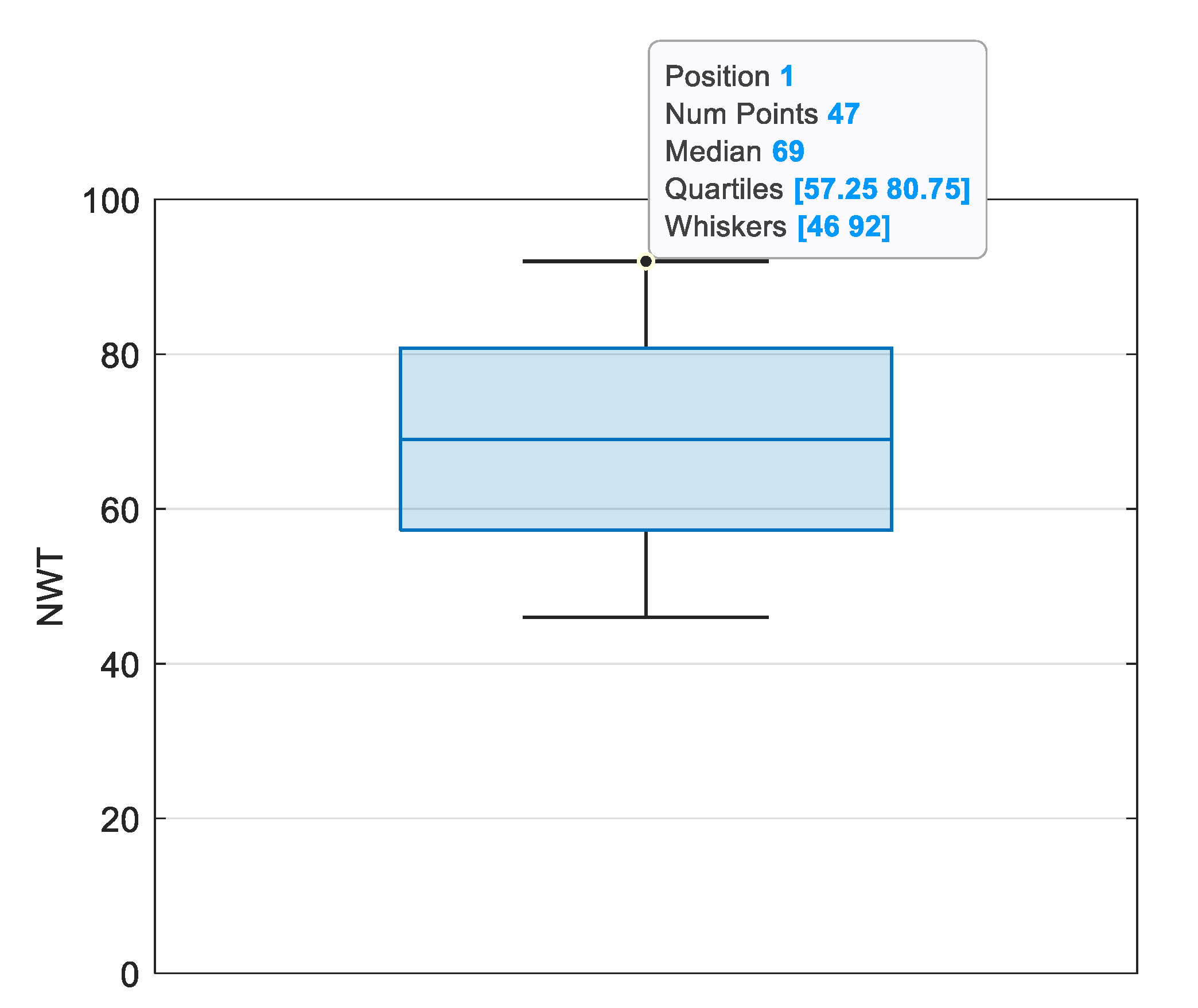
This case, similar to CASE 2, is a WFLE case where WTs located at locations # 1, 5, 26, 35, 50, 55, 80 and 83 are kept fixed. Here, the number of prefixed WTs has increased from 4 to 8 compared to CASE 2, which makes solving the problem more complicated. In this case, no constraints are imposed on NWT, which means that it follows the default range of 1 < NWT < 100. The proposed MOEA/IGD-NS/TA2 approach obtained solutions are represented in Figure 16. In total, 47 solutions have been found with different NWT ranging from 46 to 92, as shown in the box plot of Figure 17.

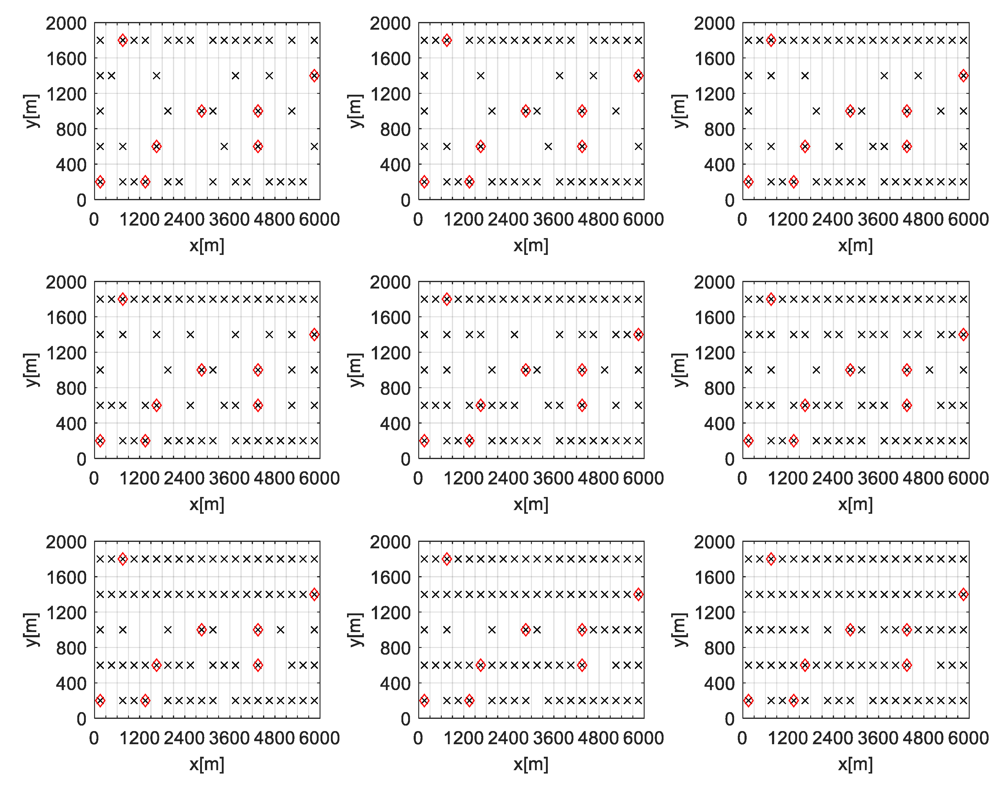
Nine selected results among the obtained ones where NWT ranges from the least to the highest are tabulated in

Table 5. Some selected layouts obtained for CASE 4.

Solution #	NWT	${\mathit{P}}_{\mathit{t}\mathit{o}\mathit{t}\mathit{a}\mathit{l}}$ [MW]	$\mathit{\eta }$ [%]	$\mathit{C}\mathit{f}$ [%]
1	46	20.57	89.83	29.81
2	52	23.03	88.96	29.52
3	58	25.39	87.93	29.18
4	63	27.25	86.89	28.84
5	69	29.34	85.43	28.35
6	75	31.38	84.06	27.90
7	81	33.36	82.73	27.45
8	86	34.94	81.62	27.09
9	92	36.78	80.32	26.66

, and their corresponding optimal layouts are represented in Figure 18. The following comments can be made from Table 5 and Figure 18:

▪

The selected solutions have 46, 52, 58, 63, 69, 75, 81 and 86 WTs, respectively.

▪

The first layout obtained with NWT = 46 has the highest $\eta$ (89.83%) and the lowest $P_{total}$ (20.57 MW).

▪

The last layout obtained with NWT = 92 has the lowest $\eta$ (80.32%) and the highest $P_{total}$ (36.78 MW).

▪

The $Cf$ varies between 26.66% and 29.81%, which is acceptable since they fall between 20% and 50%.

▪

In all the obtained solutions, WTs were located at the prefixed locations (locations # 1, 5, 26, 35, 50, 55, 80 and 83), as shown in Figure 18.

4.2.5. CASE 5

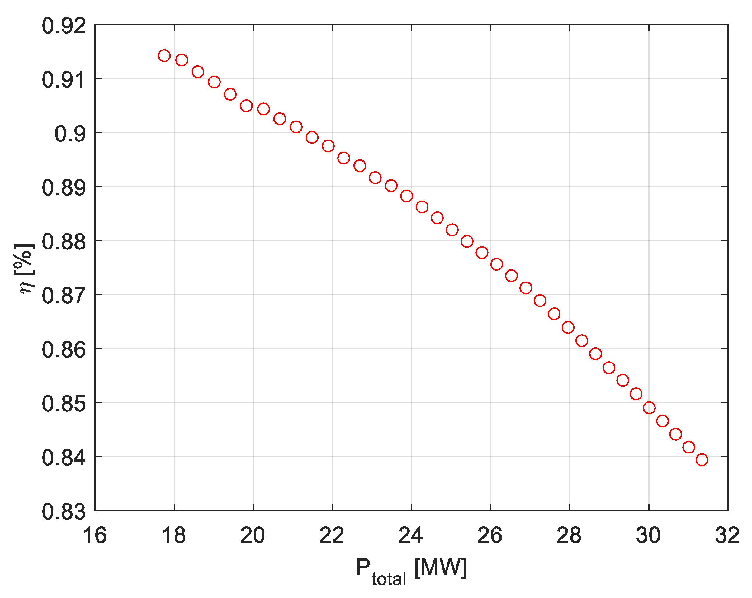
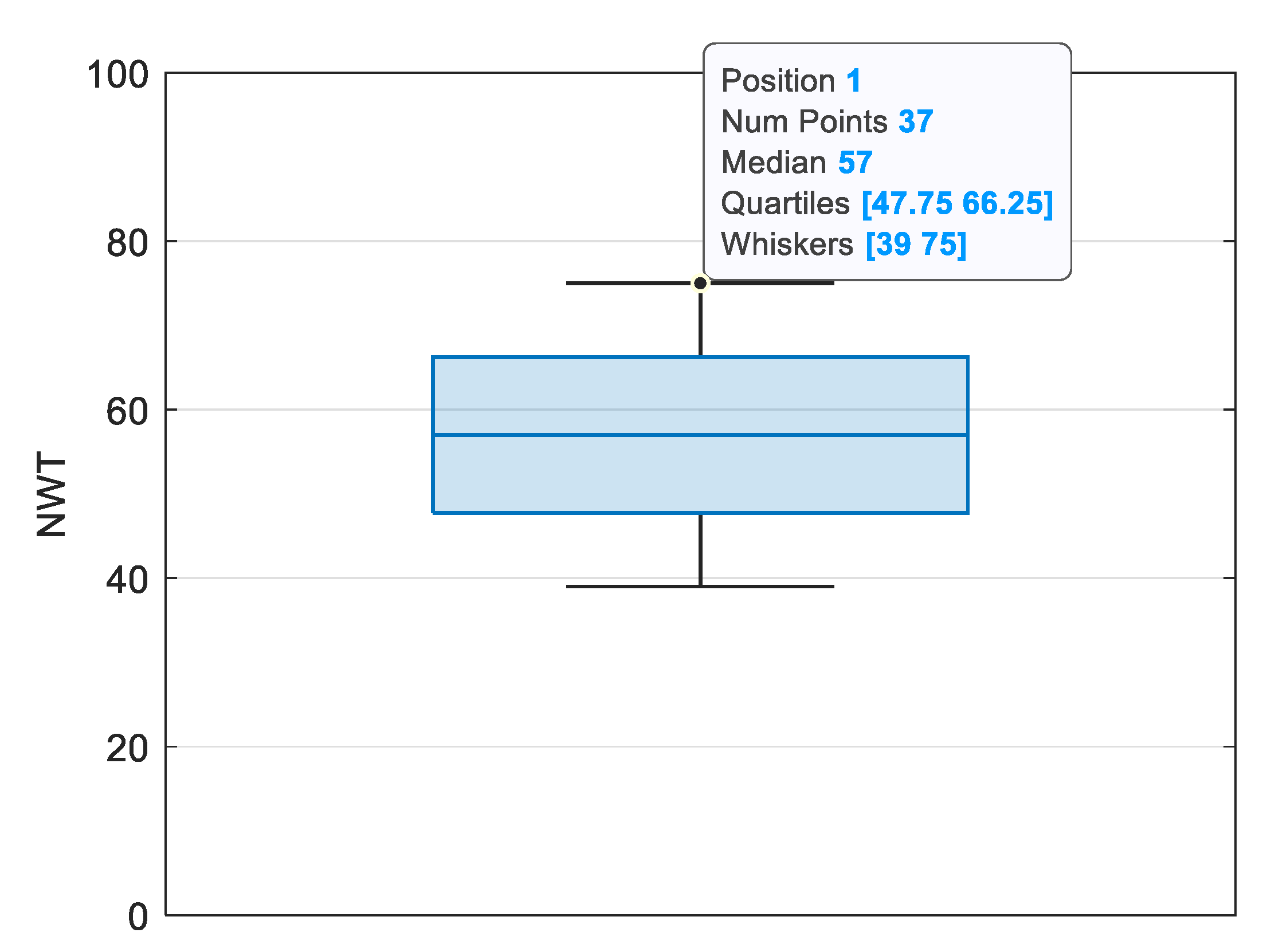
This case is similar to CASE 4, with the additional constraint of NWT range: 25 < NWT < 75. The proposed MOEA/IGD-NS/TA2 approach solutions are represented in Figure 19. In total, 37 solutions have been found with different NWT ranging from 39 to 75, as shown in the box plot of Figure 20.

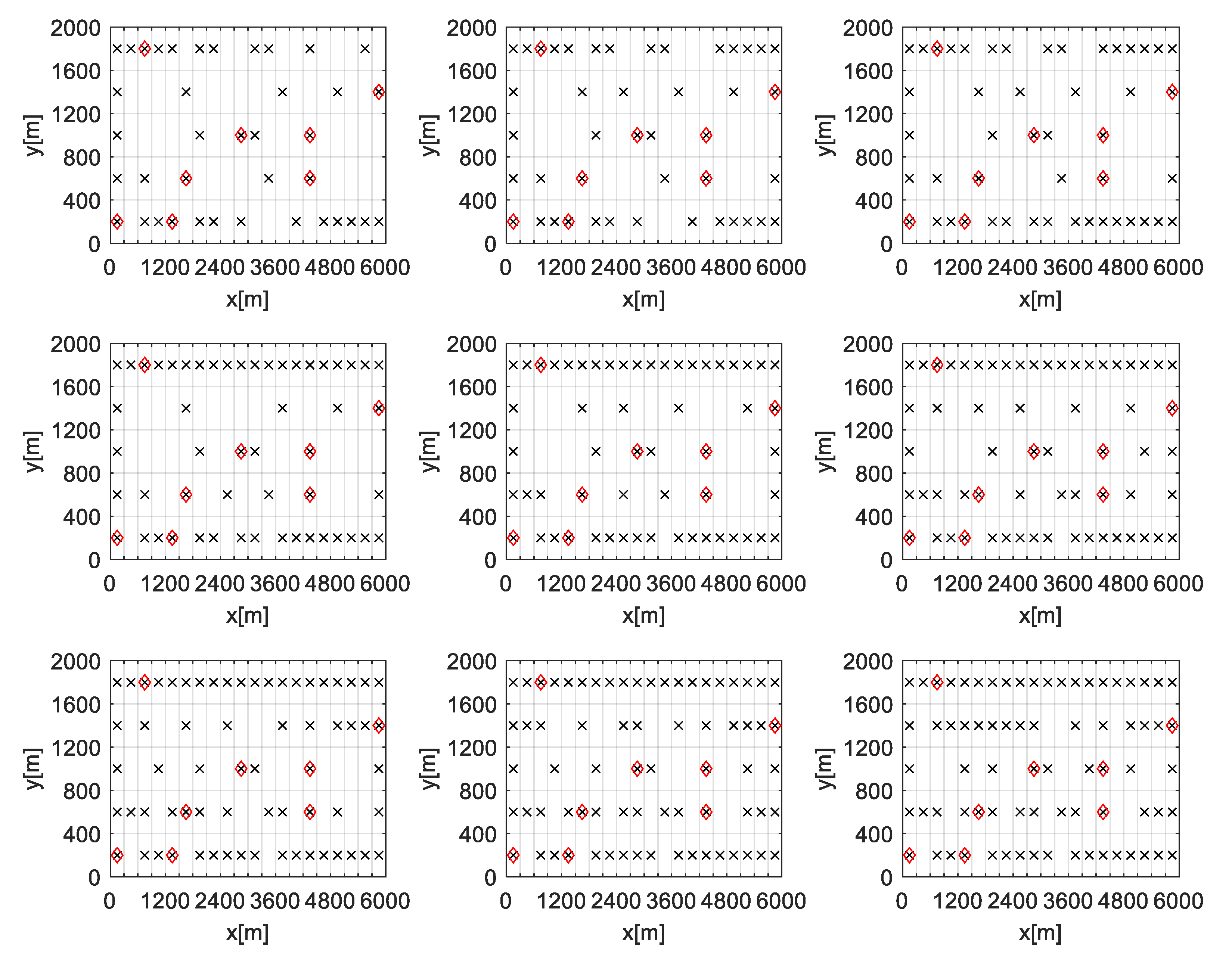
Nine selected results among the obtained ones where NWT ranges from the least value to the greatest one are tabulated in

Table 6. Some selected layouts obtained for CASE 5.

Solution #	NWT	${\mathit{P}}_{\mathit{t}\mathit{o}\mathit{t}\mathit{a}\mathit{l}}$ [MW]	$\mathit{\eta }$ [%]	$\mathit{C}\mathit{f}$ [%]
1	39	17.75	91.43	30.34
2	44	19.82	90.50	30.03
3	48	21.48	89.91	29.84
4	53	23.49	89.02	29.54
5	57	25.03	88.20	29.27
6	62	26.89	87.12	28.91
7	66	28.30	86.15	28.59
8	71	30.01	84.91	28.18
9	75	31.34	83.94	27.86

. Their corresponding optimal layouts are represented in Figure 21. The following comments can be made to summarize the obtained results:

▪

The selected solutions have 39, 44, 48, 53, 57, 62, 66, 71 and 75 WTs, respectively.

▪

The first layout obtained with NWT = 39 has the highest $\eta$ (91.43%) and the lowest $P_{total}$ (17.75 MW).

▪

The last layout obtained with NWT = 75 has the lowest $\eta$ (83.94%) and the highest $P_{total}$ (27.86 MW).

▪

The $Cf$ varies between 27.86% and 30.34%, within the acceptable range of 20–50%.

▪

In all the obtained solutions, WTs were located at the locations fixed by the designer/planner (locations # 1, 5, 26, 35, 50, 55, 80 and 83), as shown in Figure 21.

▪

The obtained values of NWT are between 25 and 75 as imposed by the designer/planner.

4.2.6. CASE 6

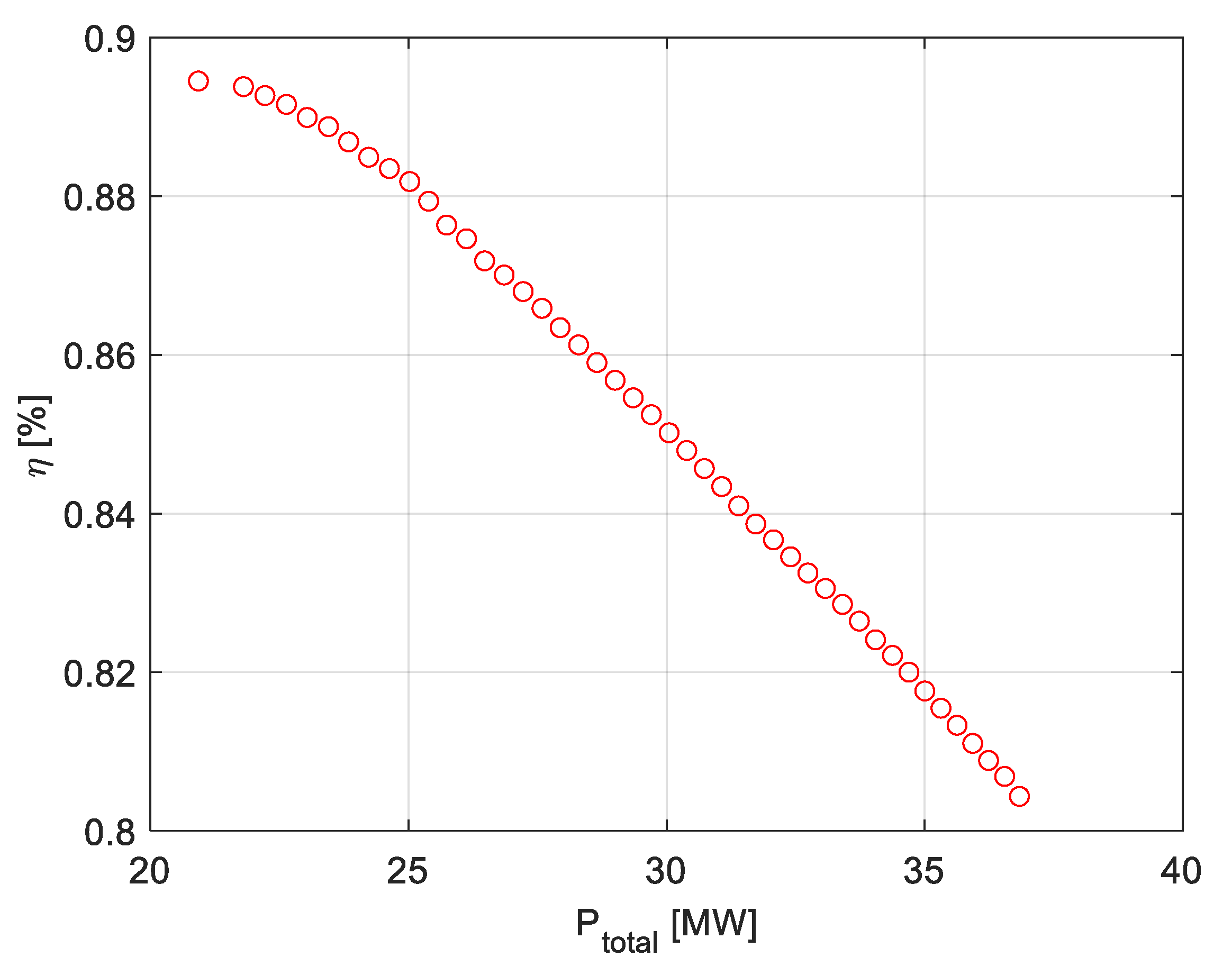
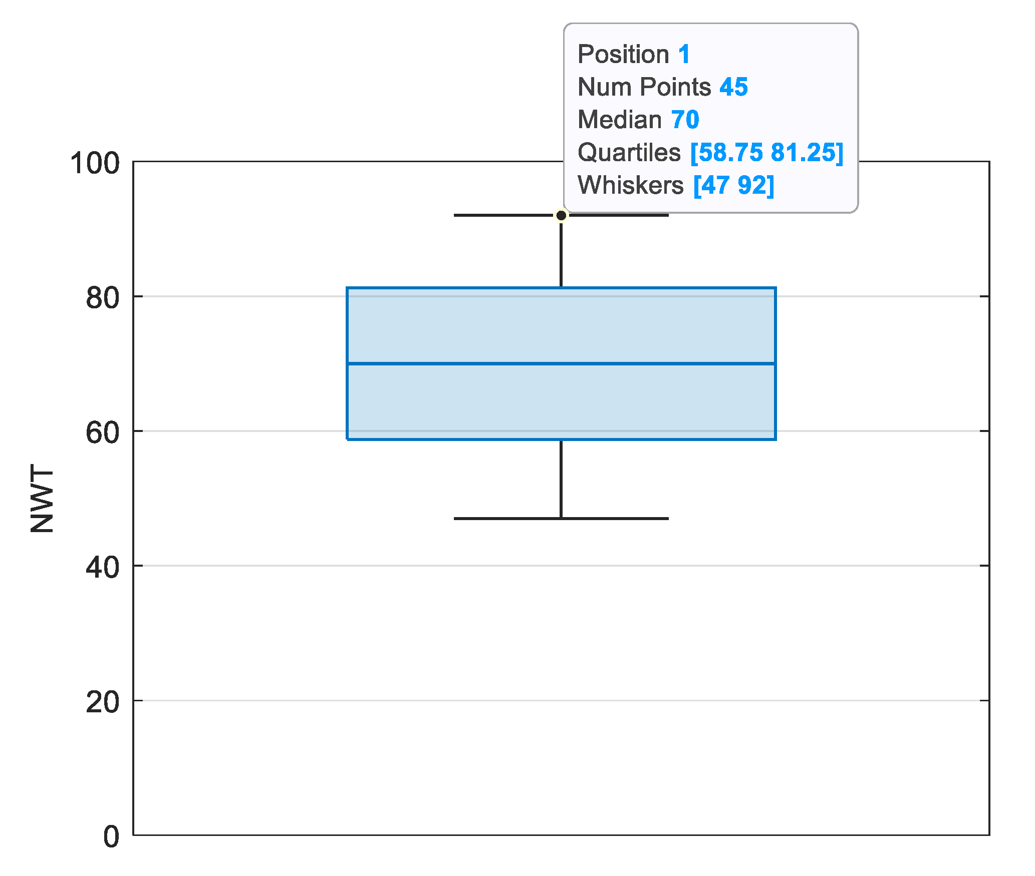
This sixth and last investigated case is a WFLE problem where WTs located at locations # 1, 5, 10, 15, 24, 40, 47, 68, 75, 80, 81, 85 and 89 are fixed. Here, the number of prefixed WTs has increased to 13, from 4 and 8 of CASE 2 and CASE 4, respectively. This makes the problem even more complicated than CASE 2 and CASE 4. No constraints are imposed on NWT (i.e., 1 < NWT < 100) in Case 6. The proposed MOEA/IGD-NS/TA2 approach has been run for this sixth case, and the obtained solutions are represented in Figure 22. The obtained PF comprises 45 solutions with different NWT, ranging from 47 to 92, as shown in the box plot of Figure 23.

Nine selected results among the obtained ones where NWT ranges from the least to the greatest are tabulated in

Table 7. Some selected layouts obtained for CASE 6.

Solution #	NWT	${\mathit{P}}_{\mathit{t}\mathit{o}\mathit{t}\mathit{a}\mathit{l}}$ [MW]	$\mathit{\eta }$ [%]	$\mathit{C}\mathit{f}$ [%]
1	47	20.93	89.45	29.69
2	54	23.84	88.68	29.43
3	59	25.74	87.63	29.08
4	65	27.94	86.34	28.65
5	70	29.70	85.24	28.29
6	76	31.73	83.87	27.83
7	81	33.41	82.85	27.50
8	87	35.32	81.54	27.06
9	92	36.84	80.43	26.69

. Their corresponding optimal layouts are represented in Figure 24. The key features of the obtained solutions are as follows:

▪

The selected solutions have 47, 54, 59, 65, 70, 76, 81, 87 and 92 WTs, respectively.

▪

The first layout obtained with NWT = 47 has the highest $\eta$ (89.45%) and the lowest $P_{total}$ (20.93 MW).

▪

The last layout obtained with NWT = 92 has the lowest $\eta$ (80.43%) and the highest $P_{total}$ (36.84 MW).

▪

The $Cf$ varies between 26.69% and 29.69%, which is acceptable since they fall between 20% and 50%.

▪

Although 13 WTs are prefixed at locations # 1, 5, 10, 15, 24, 40, 47, 68, 75, 80, 81, 85 and 89, all the obtained solutions have WTs at those prefixed locations, as shown in Figure 24, proving the robustness of the proposed approach.

4.3. Comparative Study

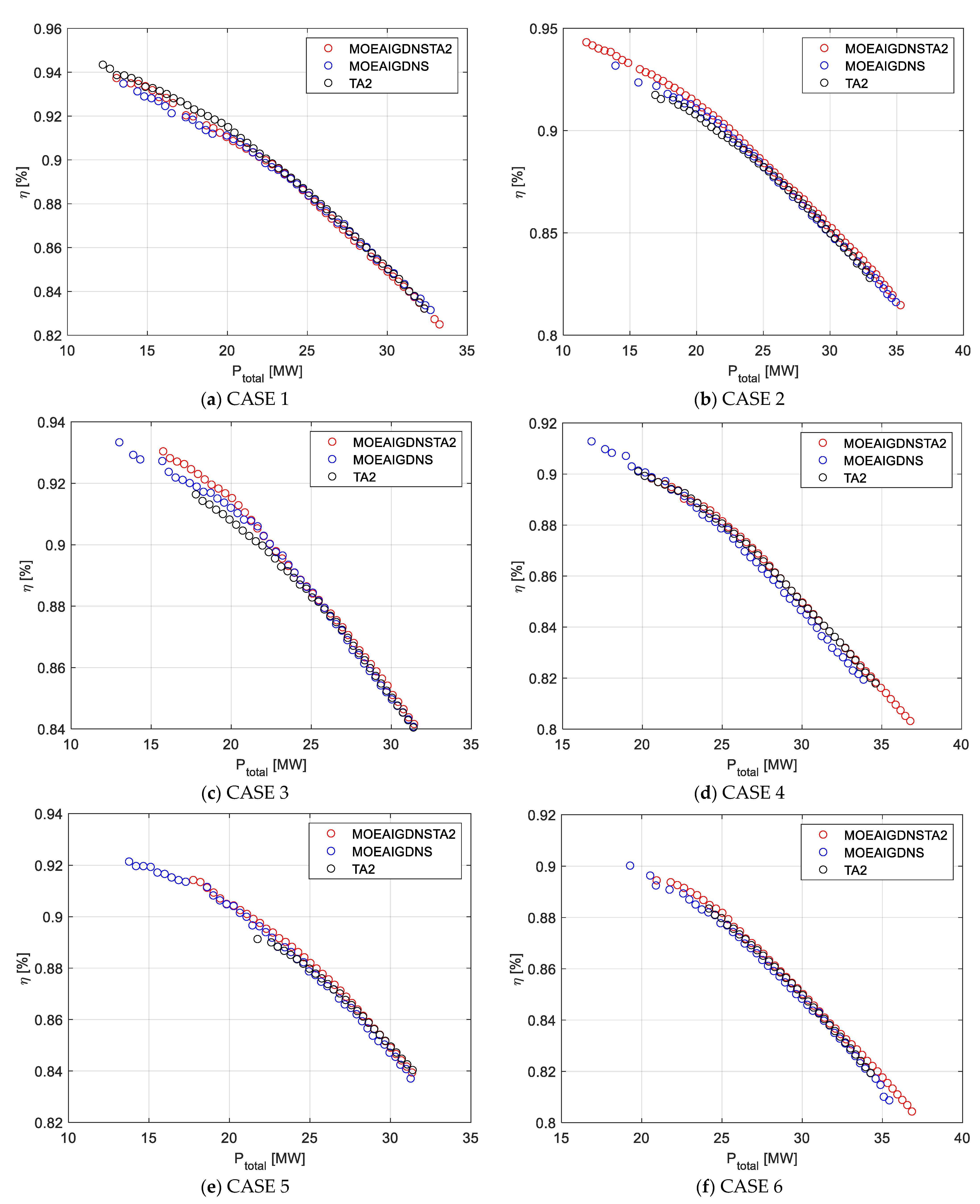
The results obtained using the proposed MOEA/IGD-NS/TA2 approach are compared with those obtained using MOEA/IGD-NS and Two_Arch2 algorithms, as shown in Figure 25. Furthermore, the C-metric which determines how good a PF obtained from one algorithm dominates a PF obtained by another algorithm and vice versa is used to compare different algorithms. The obtained C-metric values for all the cases are given in

Table 8. C-metric values obtained for all cases.

	C (MOEA/IGD-NS/TA2, MOEA/IGD-NS)	C (MOEA/IGD-NS, MOEA/IGD-NS/TA2)	C (MOEA/IGD-NS/TA2, Two_Arch2)	C (Two_Arch2, MOEA/IGD-NS/TA2)
CASE 1	0.5714	0.3750	0.9184	0.0377
CASE 2	0.0000	0.9804	0.0000	1.0000
CASE 3	0.1429	0.8444	0.0000	1.0000
CASE 4	0.0851	0.7727	0.1489	0.7857
CASE 5	0.0270	0.8182	0.1622	0.7692
CASE 6	0.0000	0.9524	0.0000	1.0000

.

It can be noticed from these Figure 25 and Table 8 that the proposed MOEA/IGD-NS/TA2 is a very competitive algorithm to solve the WFLO/E problem. This is truer in complex cases like CASE 2, CASE 3, CASE 4, CASE 5 and CASE 6, where the problem is more complicated due to the additional imposed constraints. For example, for CASE 2, CASE 3 and and CASE 4, all the solutions found by the Two_Arch2 are dominated by (or equal to) the solution found by solutions found by MOEA/IGD-NS/TA2 because the C-metric is equal to 1. Another example is for CASE 2 and CASE 6 all the solutions found usingMOEA/IGD-NS/TA2 dominate (in the strong sense) the solutions found using MOEA/IGD-NS.

5. Conclusions

This paper proposes a new multi-objective EA-based algorithm to solve the WFLO/E problem. Two algorithms, the MOEA/IGD-NS and Two_Arch2, are combined to obtain the more efficient and robust MOEA/IGD-NS/TA2 approach. The WFLO problem has been formulated as a discrete multi-objective optimization problem. More constraints are added to investigate the expansion problem where WTs are fixed at some locations, and the number of WTs is restricted. Furthermore, a smart approach has been implemented and applied to reduce the number of design variables to simplify the problem. Six cases have been investigated, all using real/commercial WTs. The solutions found are 48, 61, 42, 47, 37 and 45 for CASE 1 through CASE 6, respectively. For CASE 1, the highest efficiency found is 93.75, whilst the highest $P_{total}$ is 33.26 MW. For CASE 2, the highest $\eta$ found is 94.32, whilst the highest $P_{total}$ is 35.28 MW. For CASE 3, the highest $\eta$ found is 93.04, whilst the highest $P_{total}$ is 31.42 MW. For CASE 4, the highest $\eta$ found is 89.83, whilst the highest $P_{total}$ is 36.78 MW. For CASE 5, the highest $\eta$ found is 91.43, whilst the highest $P_{total}$ is 27.68 MW. For CASE 6, the highest $\eta$ found is 89.45, whilst the highest $P_{total}$ is 36.84 MW. The results have shown that the designer/planner can get multiple solutions (represented by the Pareto front) with a single run, which opens the door to choosing the appropriate one for the adopted system. Finally, the results are compared with the initial two EA-based algorithms to show the superiority of the proposed approach, specifically in challenging and more complicated cases. Future studies can focus on adding more objectives to the optimization problem and investigating other types of WTs.

References

1. Gross, R.; Leach, M.; Bauen, A. Progress in renewable energy. Environ. Int. 2003, 29, 105–122. [Google Scholar] [CrossRef] [PubMed]
2. Global Wind Report 2021; Global Wind Energy Council: Brussels, Belgium, 2021; Available online: https://gwec.net/global-wind-report-2021/ (accessed on 3 November 2022).
3. Elshahed, M.; Ragab, A.; Gilany, M.; Sayed, M. Investigation of switching over-voltages with different wind farm topologies. Ain Shams Eng. J. 2021, 12, 2695–2707. [Google Scholar] [CrossRef]
4. Sabiha, N.A.; Alsharef, M.; Taha, I.B.; Elattar, E.E.; Metwaly, M.K.; Abd-Elhady, A.M. Assessment of grounding grid for enhancing wind turbine service sustainability. Ain Shams Eng. J. 2021, 12, 577–589. [Google Scholar] [CrossRef]
5. Ma, Y.; Yang, H.; Zhou, X.; Li, J.; Wen, H. The dynamic modeling of wind farms considering wake effects and its optimal distribution. In Proceedings of the 2009 World Non-Grid-Connected Wind Power Energy Conference, Nanjing, China, 24–26 September 2009. [Google Scholar] [CrossRef]
6. Abdelsalam, A.M.; El-Shorbagy, M. Optimization of wind turbines siting in a wind farm using genetic algorithm based local search. Renew. Energy 2018, 123, 748–755. [Google Scholar] [CrossRef]
7. Feng, J.; Shen, W.Z. Modelling Wind for Wind Farm Layout Optimization Using Joint Distribution of Wind Speed and Wind Direction. Energies 2015, 8, 3075–3092. [Google Scholar] [CrossRef] [Green Version]
8. Lee, G.; Ding, Y.; Genton, M.G.; Xie, L. Power Curve Estimation with Multivariate Environmental Factors for Inland and Offshore Wind Farms. J. Am. Stat. Assoc. 2015, 110, 56–67. [Google Scholar] [CrossRef] [Green Version]
9. Hou, P.; Hu, W.; Soltani, M.; Chen, C.; Chen, Z. Combined optimization for offshore wind turbine micro siting. Appl. Energy 2017, 189, 271–282. [Google Scholar] [CrossRef]
10. Hou, P.; Enevoldsen, P.; Hu, W.; Chen, C.; Chen, Z. Offshore wind farm repowering optimization. Appl. Energy 2017, 208, 834–844. [Google Scholar] [CrossRef]
11. Emami, A.; Noghreh, P. New approach on optimization in placement of wind turbines within wind farm by genetic algorithms. Renew. Energy 2010, 35, 1559–1564. [Google Scholar] [CrossRef]
12. Grady, S.; Hussaini, M.; Abdullah, M. Placement of wind turbines using genetic algorithms. Renew. Energy 2005, 30, 259–270. [Google Scholar] [CrossRef]
13. González, J.S.; Rodriguez, A.G.G.; Mora, J.C.; Santos, J.R.; Payan, M.B. Optimization of wind farm turbines layout using an evolutive algorithm. Renew. Energy 2010, 35, 1671–1681. [Google Scholar] [CrossRef]
14. Bilbao, M.; Alba, E. Simulated Annealing for Optimization of Wind Farm Annual Profit. In Proceedings of the 2009 2nd International Symposium on Logistics and Industrial Informatics, Linz, Austria, 10–12 September 2009. [Google Scholar] [CrossRef]
15. Kusiak, A.; Song, Z. Design of wind farm layout for maximum wind energy capture. Renew. Energy 2010, 35, 685–694. [Google Scholar] [CrossRef]
16. Wagner, M.; Neumann, F.; Kalyan, V.; O’Reilly, U. Optimizing the Layout of 1000 Wind Turbines. Eur. Wind Energy Assoc. 2011, 47–51. [Google Scholar]
17. Ozturk, U.A.; Norman, B. Heuristic methods for wind energy conversion system positioning. Electr. Power Syst. Res. 2004, 70, 179–185. [Google Scholar] [CrossRef]
18. Eroğlu, Y.; Seçkiner, S.U. Wind farm layout optimization using particle filtering approach. Renew. Energy 2013, 58, 95–107. [Google Scholar] [CrossRef]
19. Ramli, M.A.M.; Bouchekara, H.R.E.H. Wind Farm Layout Optimization Considering Obstacles Using a Binary Most Valuable Player Algorithm. IEEE Access 2020, 8, 131553–131564. [Google Scholar] [CrossRef]
20. Li, W.W.; Özcan, E.; John, R. Multi-objective evolutionary algorithms and hyper-heuristics for wind farm layout optimisation. Renew. Energy 2017, 105, 473–482. [Google Scholar] [CrossRef] [Green Version]
21. Bansal, J.C.; Farswan, P.; Nagar, A.K. Design of wind farm layout with non-uniform turbines using fitness difference based BBO. Eng. Appl. Artif. Intell. 2018, 71, 45–59. [Google Scholar] [CrossRef]
22. Sun, H.; Yang, H.; Gao, X. Investigation into spacing restriction and layout optimization of wind farm with multiple types of wind turbines. Energy 2019, 168, 637–650. [Google Scholar] [CrossRef]
23. Long, H.; Li, P.; Gu, W. A data-driven evolutionary algorithm for wind farm layout optimization. Energy 2020, 208, 118310. [Google Scholar] [CrossRef]
24. Alham, M.; Gad, M.F.; Ibrahim, D.K. Potential of wind energy and economic assessment in Egypt considering optimal hub height by equilibrium optimizer. Ain Shams Eng. J. 2022, 14, 101816. [Google Scholar] [CrossRef]
25. Şişbot, S.; Turgut, Ö.; Tunç, M.; Çamdalı, Ü. Optimal positioning of wind turbines on Gökçeada using multi-objective genetic algorithm. Wind. Energy 2010, 13, 297–306. [Google Scholar] [CrossRef]
26. Biswas, P.P.; Suganthan, P.; Amaratunga, G.A. Decomposition based multi-objective evolutionary algorithm for windfarm layout optimization. Renew. Energy 2018, 115, 326–337. [Google Scholar] [CrossRef]
27. Zergane, S.; Smaili, A.; Masson, C. Optimization of wind turbine placement in a wind farm using a new pseudo-random number generation method. Renew. Energy 2018, 125, 166–171. [Google Scholar] [CrossRef]
28. Chen, Y.; Li, H.; Jin, K.; Song, Q. Wind farm layout optimization using genetic algorithm with different hub height wind turbines. Energy Convers. Manag. 2013, 70, 56–65. [Google Scholar] [CrossRef]
29. Chen, K.; Song, M.; Zhang, X.; Wang, S. Wind turbine layout optimization with multiple hub height wind turbines using greedy algorithm. Renew. Energy 2016, 96, 676–686. [Google Scholar] [CrossRef]
30. Al-Addous, M.; Jaradat, M.; Albatayneh, A.; Wellmann, J.; Al Hmidan, S. The Significance of Wind Turbines Layout Optimization on the Predicted Farm Energy Yield. Atmosphere 2020, 11, 117. [Google Scholar] [CrossRef] [Green Version]
31. Pérez-Aracil, J.; Casillas-Pérez, D.; Jiménez-Fernández, S.; Prieto-Godino, L.; Salcedo-Sanz, S. A versatile multi-method ensemble for wind farm layout optimization. J. Wind. Eng. Ind. Aerodyn. 2022, 225, 104991. [Google Scholar] [CrossRef]
32. Hussain, M.N.; Shaukat, N.; Ahmad, A.; Abid, M.; Hashmi, A.; Rajabi, Z.; Tariq, M.A.U.R. Effective Realization of Multi-Objective Elitist Teaching–Learning Based Optimization Technique for the Micro-Siting of Wind Turbines. Sustainability 2022, 14, 8458. [Google Scholar] [CrossRef]
33. Hou, P.; Zhu, J.; Ma, K.; Yang, G.; Hu, W.; Chen, Z. A review of offshore wind farm layout optimization and electrical system design methods. J. Mod. Power Syst. Clean Energy 2019, 7, 975–986. [Google Scholar] [CrossRef] [Green Version]
34. Deb, K.; Pratap, A.; Agarwal, S.; Meyarivan, T. A fast and elitist multiobjective genetic algorithm: NSGA-II. IEEE Trans. Evol. Comput. 2002, 6, 182–197. [Google Scholar] [CrossRef] [Green Version]
35. Zitzler, E.; Laumanns, M.; Thiele, L. SPEA2: Improving the Strength Pareto Evolutionary Algorithm; TIK-Report; ETH Zurich, Computer Engineering and Networks Laboratory: Zurich, Switzerland, 2001; Volume 103. [Google Scholar] [CrossRef]
36. Zhang, H.; Zhou, A.; Song, S.; Zhang, Q.; Gao, X.-Z.; Zhang, J. A Self-Organizing Multiobjective Evolutionary Algorithm. IEEE Trans. Evol. Comput. 2016, 20, 792–806. [Google Scholar] [CrossRef]
37. Denysiuk, R.; Costa, L.; Santo, I.E.; Matos, J.C. MOEA/PC: Multiobjective Evolutionary Algorithm Based on Polar Coordinates. Evol. Multi-Criterion Optim. 2015, 9018, 141–155. [Google Scholar] [CrossRef]
38. Corne, D.; Jerram, N.; Knowles, J.; Oates, M.; Martin, J. PESA-II: Region-based Selection in Evolutionary Multiobjective Optimization. In Proceedings of the GECCO’01: The 3rd Annual Conference on Genetic and Evolutionary Computation, San Francisco, CA, USA, 7–11 July 2001; pp. 283–290. [Google Scholar] [CrossRef]
39. Sedarous, S.; El-Gokhy, S.M.; Sallam, E. Multi-swarm multi-objective optimization based on a hybrid strategy. Alex. Eng. J. 2018, 57, 1619–1629. [Google Scholar] [CrossRef]
40. Laumanns, M.; Thiele, L.; Deb, K.; Zitzler, E. Combining Convergence and Diversity in Evolutionary Multiobjective Optimization. Evol. Comput. 2002, 10, 263–282. [Google Scholar] [CrossRef]
41. Hadka, D.; Reed, P. Borg: An Auto-Adaptive Many-Objective Evolutionary Computing Framework. Evol. Comput. 2013, 21, 231–259. [Google Scholar] [CrossRef]
42. Wang, G.; Jiang, H. Fuzzy-Dominance and Its Application in Evolutionary Many Objective Optimization. In Proceedings of the 2007 International Conference on Computational Intelligence and Security Workshops (CISW 2007), Harbin, China, 15–19 December 2007; pp. 195–198. [Google Scholar] [CrossRef]
43. Elarbi, M.; Bechikh, S.; Gupta, A.; Ben Said, L.; Ong, Y.-S. A New Decomposition-Based NSGA-II for Many-Objective Optimization. IEEE Trans. Syst. Man Cybern. Syst. 2018, 48, 1191–1210. [Google Scholar] [CrossRef]
44. Zou, X.; Chen, Y.; Liu, M.; Kang, L. A New Evolutionary Algorithm for Solving Many-Objective Optimization Problems. IEEE Trans. Syst. Man Cybern. Part B (Cybern.) 2008, 38, 1402–1412. [Google Scholar] [CrossRef] [Green Version]
45. di Pierro, F.; Khu, S.-T.; Savic, D.A. An Investigation on Preference Order Ranking Scheme for Multiobjective Evolutionary Optimization. IEEE Trans. Evol. Comput. 2007, 11, 17–45. [Google Scholar] [CrossRef]
46. Zhang, X.; Tian, Y.; Jin, Y. A Knee Point-Driven Evolutionary Algorithm for Many-Objective Optimization. IEEE Trans. Evol. Comput. 2015, 19, 761–776. [Google Scholar] [CrossRef]
47. Yang, S.; Li, M.; Liu, X.; Zheng, J. A Grid-Based Evolutionary Algorithm for Many-Objective Optimization. IEEE Trans. Evol. Comput. 2013, 17, 721–736. [Google Scholar] [CrossRef]
48. Deb, K.; Jain, H. An Evolutionary Many-Objective Optimization Algorithm Using Reference-Point-Based Nondominated Sorting Approach, Part I: Solving Problems with Box Constraints. IEEE Trans. Evol. Comput. 2014, 18, 577–601. [Google Scholar] [CrossRef]
49. Li, K.; Deb, K.; Zhang, Q.; Kwong, S. An Evolutionary Many-Objective Optimization Algorithm Based on Dominance and Decomposition. IEEE Trans. Evol. Comput. 2015, 19, 694–716. [Google Scholar] [CrossRef]
50. Zhang, Q.; Li, H. MOEA/D: A Multiobjective Evolutionary Algorithm Based on Decomposition. IEEE Trans. Evol. Comput. 2007, 11, 712–731. [Google Scholar] [CrossRef]
51. Marghny, M.; Zanaty, E.A.; Dukhan, W.H.; Reyad, O. A hybrid multi-objective optimization algorithm for software requirement problem. Alex. Eng. J. 2022, 61, 6991–7005. [Google Scholar] [CrossRef]
52. Cheng, R.; Jin, Y.; Olhofer, M.; Sendhoff, B. A Reference Vector Guided Evolutionary Algorithm for Many-Objective Optimization. IEEE Trans. Evol. Comput. 2016, 20, 773–791. [Google Scholar] [CrossRef]
53. Yuan, Y.; Xu, H.; Wang, B.; Zhang, B.; Yao, X. Balancing Convergence and Diversity in Decomposition-Based Many-Objective Optimizers. IEEE Trans. Evol. Comput. 2016, 20, 180–198. [Google Scholar] [CrossRef]
54. Wang, R.; Purshouse, R.C.; Fleming, P.J. Preference-Inspired Coevolutionary Algorithms for Many-Objective Optimization. IEEE Trans. Evol. Comput. 2013, 17, 474–494. [Google Scholar] [CrossRef]
55. Beume, N.; Naujoks, B.; Emmerich, M. SMS-EMOA: Multiobjective selection based on dominated hypervolume. Eur. J. Oper. Res. 2007, 181, 1653–1669. [Google Scholar] [CrossRef]
56. Gómez, R.H.; Coello, C.A.C. Improved Metaheuristic Based on the R2 Indicator for Many-Objective Optimization. In Proceedings of the GECCO’15: Genetic and Evolutionary Computation Conference, Madrid, Spain, 11–15 July 2015; pp. 679–686. [Google Scholar] [CrossRef]
57. Bader, J.; Zitzler, E. HypE: An Algorithm for Fast Hypervolume-Based Many-Objective Optimization. Evol. Comput. 2011, 19, 45–76. [Google Scholar] [CrossRef]
58. Tian, Y.; Zhang, X.; Cheng, R.; Jin, Y. A multi-objective evolutionary algorithm based on an enhanced inverted generational distance metric. In Proceedings of the 2016 IEEE Congress on Evolutionary Computation (CEC), Vancouver, BC, Canada, 24–29 July 2016; pp. 5222–5229. [Google Scholar] [CrossRef]
59. Wang, H.; Jiao, L.; Yao, X. Two_Arch2: An Improved Two-Archive Algorithm for Many-Objective Optimization. IEEE Trans. Evol. Comput. 2015, 19, 524–541. [Google Scholar] [CrossRef]
60. Bouchekara, H.R.E.-H.; Javaid, M.S.; Shaaban, Y.A.; Shahriar, M.S.; Ramli, M.A.M.; Latreche, Y. Decomposition based multiobjective evolutionary algorithm for PV/Wind/Diesel Hybrid Microgrid System design considering load uncertainty. Energy Rep. 2021, 7, 52–69. [Google Scholar] [CrossRef]
61. Markarian, S.; Fazelpour, F.; Markarian, E. Optimization of wind farm layout considering wake effect and multiple parameters. Environ. Prog. Sustain. Energy 2019, 38, 13193. [Google Scholar] [CrossRef]
62. Yeghikian, M.; Ahmadi, A.; Dashti, R.; Esmaeilion, F.; Mahmoudan, A.; Hoseinzadeh, S.; Garcia, D.A. Wind Farm Layout Optimization with Different Hub Heights in Manjil Wind Farm Using Particle Swarm Optimization. Appl. Sci. 2021, 11, 9746. [Google Scholar] [CrossRef]
63. Arreyndip, N.A.; Joseph, E. Small 500 kW onshore wind farm project in Kribi, Cameroon: Sizing and checkers layout optimization model. Energy Rep. 2018, 4, 528–535. [Google Scholar] [CrossRef]
64. El Mokhi, C.; Addaim, A. Optimization of Wind Turbine Interconnections in an Offshore Wind Farm Using Metaheuristic Algorithms. Sustainability 2020, 12, 5761. [Google Scholar] [CrossRef]
65. Holmes, J.D.; Bekele, S.A. Wind Loading of Structures; CRC Press: Boca Raton, FL, USA, 2020. [Google Scholar]
66. Shao, Z.; Wu, Y.; Li, L.; Han, S.; Liu, Y. Multiple Wind Turbine Wakes Modeling Considering the Faster Wake Recovery in Overlapped Wakes. Energies 2019, 12, 680. [Google Scholar] [CrossRef] [Green Version]
67. Beşkirli, M.; Koç, I.; Haklı, H.; Kodaz, H. A new optimization algorithm for solving wind turbine placement problem: Binary artificial algae algorithm. Renew. Energy 2018, 121, 301–308. [Google Scholar] [CrossRef]
68. Hakli, H. A new approach for wind turbine placement problem using modified differentialevolution algorithm. Turk. J. Electr. Eng. Comput. Sci. 2019, 27, 4659–4672. [Google Scholar] [CrossRef]
69. Zitzler, E.; Kunzli, S. Indicator-based selection in multiobjective search. In Proceedings of the Parallel Problem Solving from Nature–PPSN VIII, International Conference on Parallel Problem Solving from Nature, Birmingham, UK, 13–17 September 2004; Yao, X., Ed.; Springer: Berlin, Germany, 2004. [Google Scholar] [CrossRef]
70. Zhou, A.; Jin, Y.; Zhang, Q.; Sendhoff, B.; Tsang, E. Combining Model-based and Genetics-based Offspring Generation for Multi-objective Optimization Using a Convergence Criterion. In Proceedings of the 2006 IEEE International Conference on Evolutionary Computation, Vancouver, BC, Canada, 16–21 July 2006; pp. 892–899. [Google Scholar] [CrossRef]
71. Van Veldhuizen, D.A.; Lamont, G.B. Multiobjective evolutionary algorithm research: A history and analysis. In Technical Report TR-98-03; Department of Electrical and Computer Engineering, Graduate School of Engineering, Air Force Institute of Technology, Wright-Patterson AFB: Dayton, OH, USA, 1998. [Google Scholar]
72. Schutze, O.; Esquivel, X.; Lara, A.; Coello, C.A.C. Using the Averaged Hausdorff Distance as a Performance Measure in Evolutionary Multiobjective Optimization. IEEE Trans. Evol. Comput. 2012, 16, 504–522. [Google Scholar] [CrossRef]
73. Zhang, X.; Tian, Y.; Cheng, R.; Jin, Y. An Efficient Approach to Nondominated Sorting for Evolutionary Multiobjective Optimization. IEEE Trans. Evol. Comput. 2015, 19, 201–213. [Google Scholar] [CrossRef] [Green Version]
74. Praditwong, K.; Yao, X. A New Multi-objective Evolutionary Optimisation Algorithm: The Two-Archive Algorithm. In 2006 International Conference on Computational Intelligence and Security; Springer: Berlin/Heidelberg, Germany, 2006; Volume 1, pp. 286–291. [Google Scholar] [CrossRef]
75. Aggarwal, C.C.; Hinneburg, A.; Keim, D.A. On the Surprising Behavior of Distance Metrics in High Dimensional Space. In Proceedings of the Database Theory—ICDT 2001; Van den Bussche, J., Vianu, V., Eds.; Springer: Berlin/Heidelberg, Germany, 2001; pp. 420–434. [Google Scholar] [CrossRef]
Figure 1. Illustration of the WFLO problem.
Sustainability 15 02525 g001
Figure 2. Illustration of the WFLE problem.
Sustainability 15 02525 g002
Figure 3. Illustration of the proposed variable reduction approaches.
Sustainability 15 02525 g003
Figure 4. Flowchart for (a) Two_Arch (b) Two_Arch2. (c) Flowchart for the implementation of the proposed mwthod to solve the WFLO/W problwm.
Sustainability 15 02525 g004
Figure 5. Wind probability distribution diagram used in this study.
Sustainability 15 02525 g005
Figure 6. Real power curve for the ‘Acciona AW82/1500 kW’ WT.
Sustainability 15 02525 g006
Figure 7. PF obtained for CASE 1.
Sustainability 15 02525 g007
Figure 8. Box plot of NWT for CASE 1.
Sustainability 15 02525 g008
Figure 9. Selected optimal wind farm layouts for CASE 1.
Sustainability 15 02525 g009
Figure 10. PF obtained for CASE 2.
Sustainability 15 02525 g010
Figure 11. Box plot of NWT for CASE 2.
Sustainability 15 02525 g011
Figure 12. Selected optimal wind farm layouts for CASE 2.
Sustainability 15 02525 g012
Figure 13. PF obtained for CASE 3.
Sustainability 15 02525 g013
Figure 14. Box plot of NWT for CASE 3.
Sustainability 15 02525 g014
Figure 15. Selected optimal wind farm layouts for CASE 3.
Sustainability 15 02525 g015
Figure 16. PF obtained for CASE 4.
Sustainability 15 02525 g016
Figure 17. Box plot of NWT for CASE 4.
Sustainability 15 02525 g017
Figure 18. Selected optimal wind farm layouts for CASE 4.
Sustainability 15 02525 g018
Figure 19. PF obtained for CASE 5.
Sustainability 15 02525 g019
Figure 20. Box plot of NWT for CASE 5.
Sustainability 15 02525 g020
Figure 21. Selected optimal wind farm layouts for CASE 5.
Sustainability 15 02525 g021
Figure 22. PF obtained for CASE 6.
Sustainability 15 02525 g022
Figure 23. Box plot of NWT for CASE 6.
Sustainability 15 02525 g023
Figure 24. Selected optimal wind farm layouts for CASE 6.
Sustainability 15 02525 g024
Figure 25. Comparison of the proposed MOEA/IGD-NS/TA2 with MOEA/IGD-NS and Two_Arch2.
Sustainability 15 02525 g025