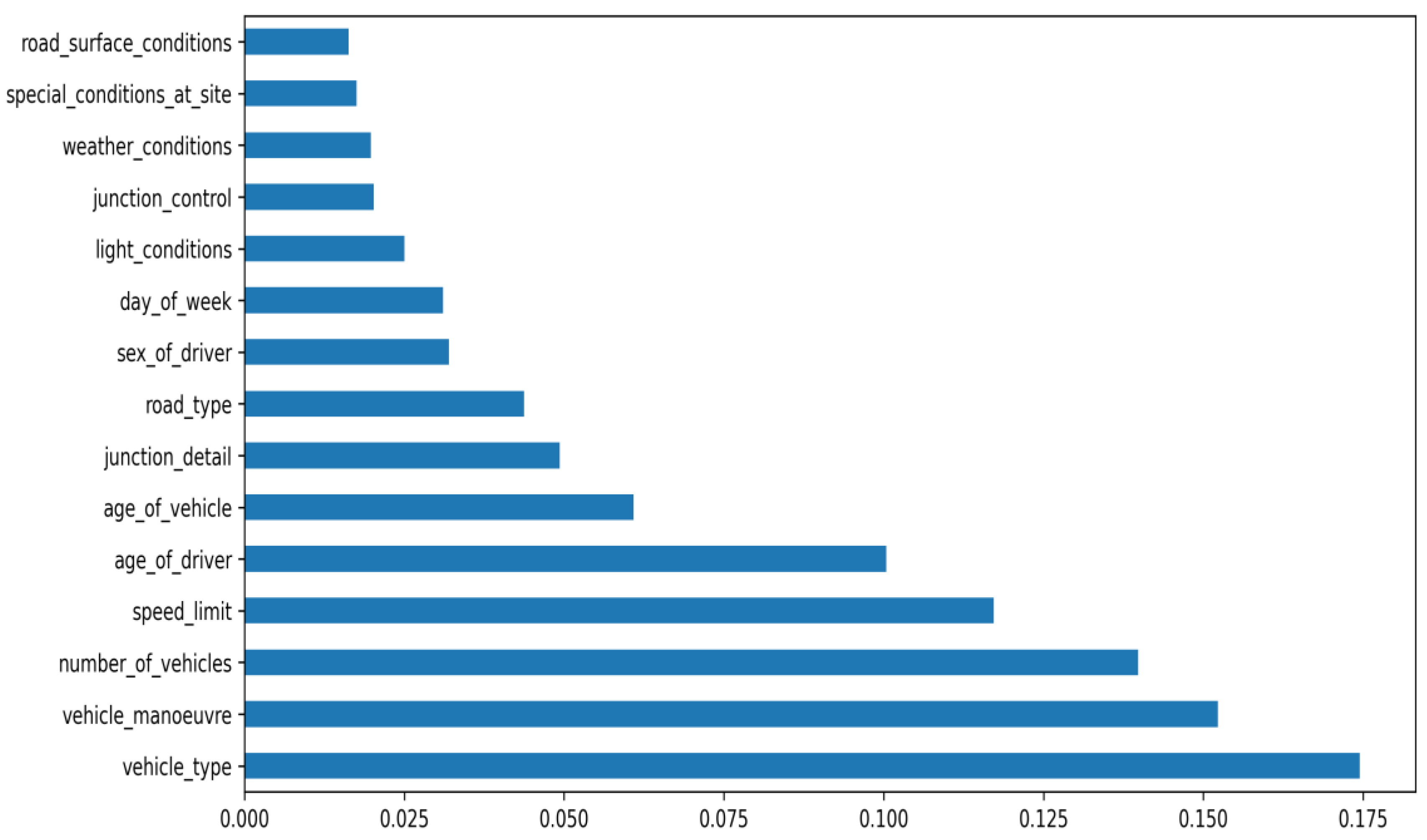
Figure 1.
The Random Forest Classifier’s bar chart for feature importance scores, displayed in ascending order.
Figure 1.
The Random Forest Classifier’s bar chart for feature importance scores, displayed in ascending order.
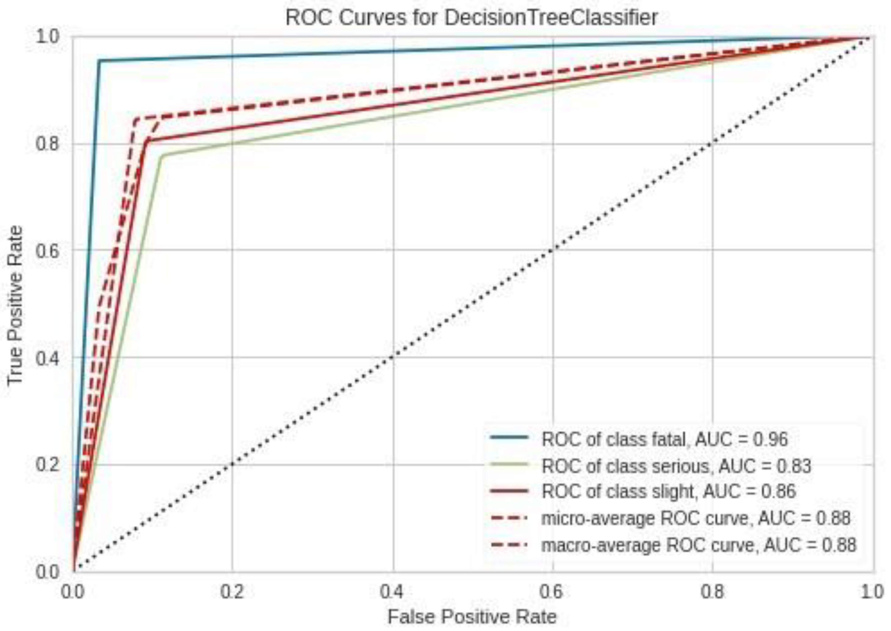
Figure 2.
Receiver Operating Characteristic (ROC) curves for each accident severity class of Decision Tree algorithm analysis result with default parameters. The area under the ROC curve is reported in the legend.
Figure 2.
Receiver Operating Characteristic (ROC) curves for each accident severity class of Decision Tree algorithm analysis result with default parameters. The area under the ROC curve is reported in the legend.
Figure 3.
Receiver Operating Characteristic (ROC) curves for each accident severity class of Decision Tree algorithm analysis result with hyper-tuning parameters. The area under the ROC curve is reported in the legend.
Figure 3.
Receiver Operating Characteristic (ROC) curves for each accident severity class of Decision Tree algorithm analysis result with hyper-tuning parameters. The area under the ROC curve is reported in the legend.
Figure 4.
Receiver Operating Characteristic (ROC) curves for each accident severity class of LightGBM algorithm analysis result with default parameters. The area under the ROC curve is reported in the legend.
Figure 4.
Receiver Operating Characteristic (ROC) curves for each accident severity class of LightGBM algorithm analysis result with default parameters. The area under the ROC curve is reported in the legend.
Figure 5.
Receiver Operating Characteristic (ROC) curves for each accident severity class of LightGBM algorithm analysis result with hyper-tuning parameters. The area under the ROC curve is reported in the legend.
Figure 5.
Receiver Operating Characteristic (ROC) curves for each accident severity class of LightGBM algorithm analysis result with hyper-tuning parameters. The area under the ROC curve is reported in the legend.
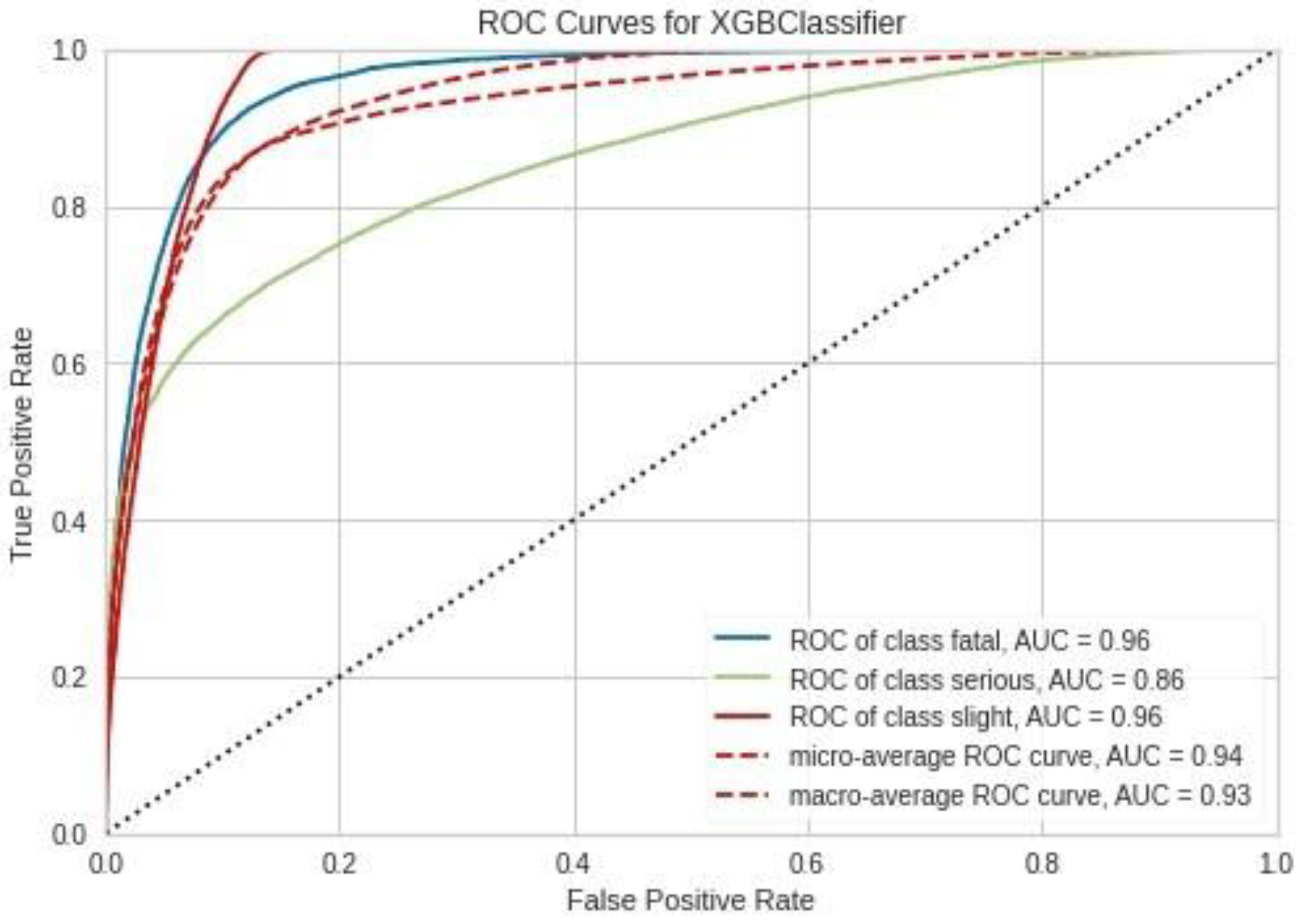
Figure 6.
Receiver Operating Characteristic (ROC) curves for each accident severity class of XGboost algorithm analysis result with default parameters. The area under the ROC curve is reported in the legend.
Figure 6.
Receiver Operating Characteristic (ROC) curves for each accident severity class of XGboost algorithm analysis result with default parameters. The area under the ROC curve is reported in the legend.
Figure 7.
Receiver Operating Characteristic (ROC) curves for each accident severity class of XGboost algorithm analysis result with hyper-tuning parameters. The area under the ROC curve is reported in the legend.
Figure 7.
Receiver Operating Characteristic (ROC) curves for each accident severity class of XGboost algorithm analysis result with hyper-tuning parameters. The area under the ROC curve is reported in the legend.
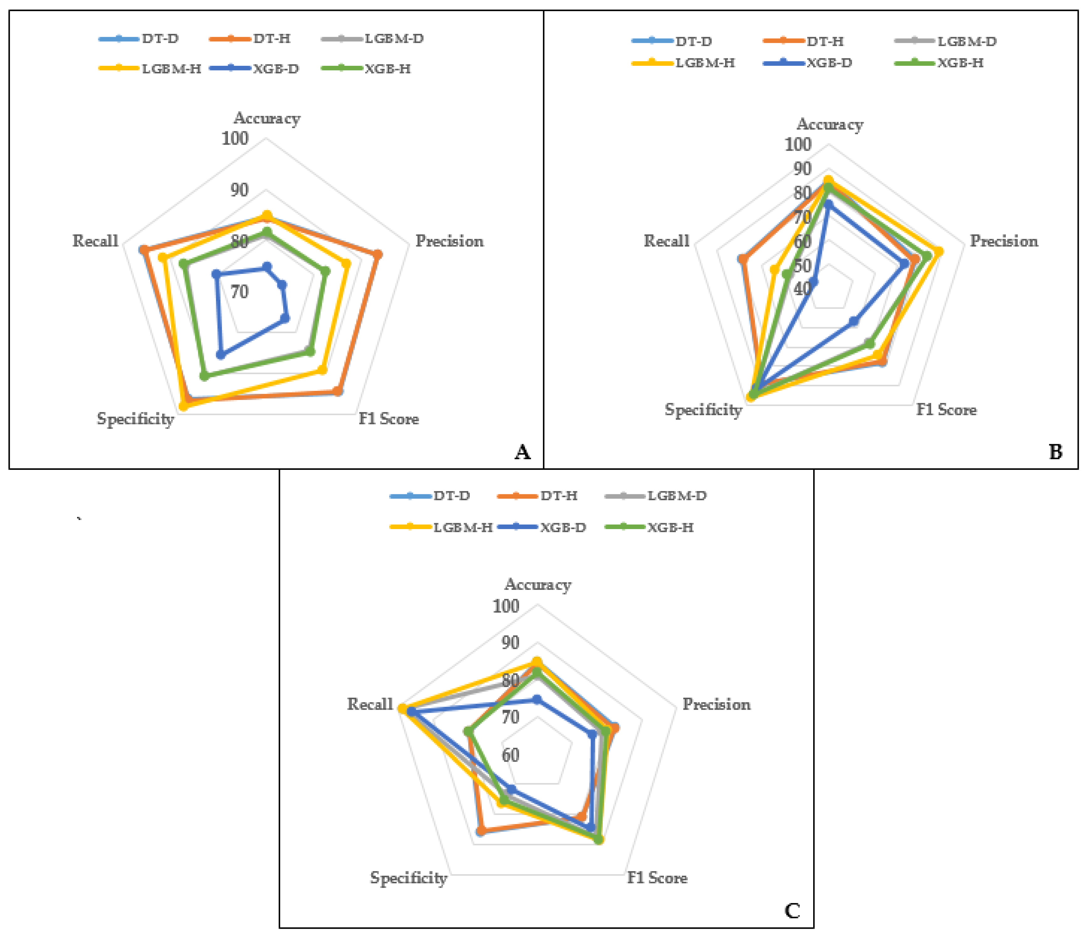
Figure 8.
Performance measures of the developed models. (A): Fatal, (B): Serious injuries and (C): Slight injuries.
Figure 8.
Performance measures of the developed models. (A): Fatal, (B): Serious injuries and (C): Slight injuries.
Table 1.
Descriptive statistics data related to traffic accident.
Table 1.
Descriptive statistics data related to traffic accident.
| Variable | Fatal | Serious | Slight | Total |
|---|
| N | % | N | % | N | % | N | % |
|---|
| Sex of driver | | | | | | | | |
| Male | 1394 | 2 | 17,121 | 20 | 67,028 | 78 | 85,543 | 63.2 |
| Female | 288 | 1 | 5099 | 16 | 27,290 | 84 | 32,677 | 24.1 |
| Not traced | 74 | 0 | 2211 | 13 | 14,947 | 87 | 17,219 | 12.7 |
| Age of driver | | | | | | | | |
| <24 | 337 | 1 | 6603 | 16 | 34,594 | 83 | 41,534 | 30.7 |
| 25–34 | 373 | 1 | 5194 | 17 | 24,567 | 82 | 30,134 | 22.2 |
| 35–44 | 294 | 1 | 4022 | 18 | 18,298 | 81 | 22,614 | 16.7 |
| 45–54 | 274 | 1 | 3679 | 19 | 15,194 | 79 | 19,147 | 14.1 |
| 55–64 | 249 | 2 | 2787 | 22 | 9877 | 76 | 12,913 | 9.5 |
| 65–74 | 124 | 2 | 1343 | 24 | 4084 | 74 | 5551 | 4.1 |
| >75 | 105 | 3 | 803 | 23 | 2651 | 74 | 3559 | 2.6 |
| Road type | | | | | | | | |
| Roundabout | 24 | 0 | 1175 | 14 | 7370 | 86 | 8569 | 6.3 |
| One way street | 5 | 0 | 418 | 13 | 2753 | 87 | 3176 | 2.3 |
| Dual carriageway | 343 | 2 | 3680 | 17 | 17,928 | 82 | 21,951 | 16.2 |
| Single carriageway | 1362 | 1 | 18,581 | 19 | 76,028 | 79 | 95,971 | 70.8 |
| Slip Road | 20 | 1 | 346 | 14 | 2141 | 85 | 2507 | 1.8 |
| Unknown | 2 | 0 | 231 | 7 | 3046 | 93 | 3279 | 2.4 |
| Speed limit | | | | | | | | |
| 20 | 63 | 0 | 2348 | 13 | 15,073 | 86 | 17,484 | 12.9 |
| 30 | 584 | 1 | 13,440 | 17 | 65,219 | 82 | 79,243 | 58.5 |
| 40 | 182 | 2 | 2451 | 20 | 9418 | 78 | 12,051 | 8.9 |
| 50 | 143 | 2 | 1163 | 20 | 4574 | 78 | 5880 | 4.3 |
| 60 | 574 | 4 | 3530 | 27 | 8981 | 69 | 13,085 | 9.7 |
| 70 | 210 | 3 | 1496 | 19 | 5990 | 78 | 7696 | 5.7 |
| Missing | 0 | 0 | 3 | 21 | 11 | 79 | 14 | 0.0 |
| Junction control | | | | | | | | |
| Authorized person | 3 | 1 | 92 | 17 | 446 | 82 | 541 | 0.4 |
| Automatic traffic signal | 96 | 1 | 2286 | 13 | 14,845 | 86 | 17,227 | 12.7 |
| Stop sign | 3 | 0 | 157 | 17 | 761 | 83 | 921 | 0.7 |
| Give way or uncontrolled | 508 | 1 | 10,950 | 18 | 49,536 | 81 | 60,994 | 45.0 |
| Not at junction or within 20 m | 1146 | 2 | 10,804 | 20 | 41,041 | 77 | 52,991 | 39.1 |
| Missing | 0 | 0 | 142 | 5 | 2637 | 95 | 2779 | 2.1 |
| Special conditions at site | | | | | | | | |
| None | 1707 | 1 | 23,549 | 18 | 104,026 | 80 | 129,282 | 95.4 |
| Roadworks | 33 | 2 | 310 | 17 | 1508 | 81 | 1851 | 1.4 |
| Others | 12 | 4 | 325 | 138 | 1216 | 457 | 1366 | 1 |
| Unknown | 4 | 0 | 247 | 8 | 2703 | 92 | 2954 | 2.2 |
| Number of vehicles | | | | | | | | |
| 1 | 496 | 2 | 5309 | 27 | 14,194 | 71 | 19,999 | 14.8 |
| 2 | 772 | 1 | 15,156 | 16 | 78,282 | 83 | 94,210 | 69.6 |
| 3–5 | 421 | 2 | 3787 | 19 | 16,136 | 79 | 20,344 | 15.0 |
| >5 | 67 | 7 | 179 | 20 | 654 | 73 | 900 | 0.7 |
| Age of vehicle | | | | | | | | |
| 0–10 | 901 | 1 | 11,296 | 17 | 54,830 | 82 | 67,027 | 49.5 |
| 11–20 years | 465 | 1 | 5678 | 18 | 25,929 | 81 | 32,072 | 23.7 |
| 21–30 years | 34 | 3 | 354 | 28 | 856 | 69 | 1244 | 0.9 |
| 31–40 years | 3 | 3 | 39 | 35 | 71 | 63 | 113 | 0.1 |
| Above 40 years | 1 | 1 | 28 | 31 | 62 | 68 | 91 | 0.1 |
| Missing | 352 | 1 | 7036 | 20 | 27,517 | 79 | 34,905 | 25.8 |
| Vehicle type | | | | | | | | |
| Pedal cycle | 119 | 1 | 3227 | 23 | 10,498 | 76 | 13,844 | 10.2 |
| Motorcycle < 500 cc | 75 | 3 | 2079 | 76 | 6698 | 221 | 8852 | 6.5 |
| Motorcycle > 500 cc | 147 | 5 | 1161 | 41 | 1504 | 53 | 2812 | 2.1 |
| Car | 1056 | 2 | 14,921 | 28 | 78,018 | 170 | 93,995 | 69.4 |
| Bus | 27 | 3 | 351 | 33 | 1668 | 164 | 2046 | 2 |
| Truck | 275 | 12 | 1992 | 57 | 8797 | 231 | 11,064 | 8.2 |
| Others | 57 | 15 | 700 | 229 | 2083 | 556 | 2840 | 2.1 |
| Vehicle manoeuvre | | | | | | | | |
| Going ahead | 1338 | 9 | 14,560 | 75 | 53,389 | 217 | 69,287 | 51 |
| Turning left/right/U | 127 | 2 | 3519 | 59 | 13,890 | 239 | 17,536 | 13 |
| Reversing | 14 | 1 | 238 | 15 | 1383 | 85 | 1635 | 1.2 |
| Parked | 98 | 2 | 1184 | 20 | 4581 | 78 | 5863 | 4.3 |
| Slowing/stopping/waiting | 65 | 1 | 1715 | 46 | 13,167 | 352 | 14,947 | 11 |
| Overtaking | 66 | 4 | 1056 | 66 | 3489 | 231 | 4611 | 3 |
| Others | 46 | 2 | 1336 | 46 | 6728 | 252 | 8110 | 6 |
| Missing | 2 | 0 | 823 | 19 | 12,639 | 181 | 13,464 | 10 |
| Day of the week | | | | | | | | |
| Monday | 267 | 2 | 2998 | 20 | 11,785 | 78 | 15,050 | 11.1 |
| Tuesday | 239 | 1 | 3333 | 18 | 15,451 | 81 | 19,023 | 14.0 |
| Wednesday | 222 | 1 | 3403 | 17 | 16,018 | 82 | 19,643 | 14.5 |
| Thursday | 242 | 1 | 3533 | 17 | 16,642 | 82 | 20,417 | 15.1 |
| Friday | 258 | 1 | 3843 | 18 | 16,920 | 80 | 21,021 | 15.5 |
| Saturday | 250 | 1 | 3900 | 18 | 17,910 | 81 | 22,060 | 16.3 |
| Sunday | 278 | 2 | 3421 | 19 | 14,540 | 80 | 18,239 | 13.5 |
| Light condition | | | | | | | | |
| Daylight: streetlights present | 1064 | 1 | 16,960 | 18 | 78,068 | 81 | 96,092 | 70.9 |
| Darkness: streetlights present and lit | 359 | 1 | 5528 | 19 | 23,773 | 80 | 29,660 | 21.9 |
| Darkness: streetlights present but unlit | 11 | 1 | 176 | 19 | 756 | 80 | 943 | 0.7 |
| Darkness: no street lighting | 293 | 5 | 1377 | 26 | 3679 | 69 | 5349 | 3.9 |
| Darkness: street lighting unknown | 29 | 1 | 390 | 11 | 2990 | 88 | 3409 | 2.5 |
| Weather conditions | | | | | | | | |
| Fine without high winds | 1473 | 1 | 19,760 | 19 | 85,416 | 80 | 106,649 | 78.7 |
| Raining without high winds | 141 | 1 | 2718 | 17 | 13,531 | 83 | 16,390 | 12.1 |
| Snowing without high winds | 0 | 0 | 37 | 16 | 189 | 84 | 226 | 0.2 |
| Fine with high winds | 37 | 2 | 426 | 22 | 1470 | 76 | 1933 | 1.4 |
| Raining with high winds | 31 | 2 | 354 | 19 | 1497 | 80 | 1882 | 1.4 |
| Snowing with high winds | 0 | 0 | 20 | 29 | 48 | 71 | 68 | 0.1 |
| Fog or mist—if hazard | 30 | 4 | 147 | 20 | 554 | 76 | 731 | 0.5 |
| Other | 33 | 1 | 548 | 13 | 3536 | 86 | 4117 | 3.0 |
| Unknown | 11 | 0 | 421 | 12 | 3025 | 88 | 3457 | 2.6 |
| Road surface conditions | | | | | | | | |
| Dry | 1215 | 1 | 17,475 | 18 | 76,887 | 80 | 95,577 | 70.6 |
| Wet/Damp | 522 | 1 | 6552 | 18 | 29,596 | 81 | 36,670 | 27.1 |
| Snow | 0 | 0 | 25 | 15 | 141 | 85 | 166 | 0.1 |
| Frost/Ice | 12 | 1 | 171 | 20 | 662 | 78 | 845 | 0.6 |
Table 2.
The Decision Tree algorithm analysis result with default parameters includes a summary of precision, recall, per-class F1-Score, specificity and the false positive rate (FPR) measurements for the three classes. The overall accuracy of the model was also measured.
Table 2.
The Decision Tree algorithm analysis result with default parameters includes a summary of precision, recall, per-class F1-Score, specificity and the false positive rate (FPR) measurements for the three classes. The overall accuracy of the model was also measured.
| Accuracy | 84.61% |
|---|
| Predicted Values |
|---|
| Value | Precision | Recall | F1-Score | Specificity | FPR |
|---|
| Fatal | 0.932518 | 0.957956 | 0.945066 | 0.962942 | 0.037058 |
| Serious | 0.779072 | 0.785760 | 0.782402 | 0.889107 | 0.110893 |
| Slight | 0.824731 | 0.795534 | 0.809869 | 0.859503 | 0.140497 |
Table 3.
The Decision Tree algorithm analysis result with hyper-tuning parameters includes a summary of precision, recall, per-class F1-Score, specificity and the false positive rate (FPR) measurements of the three classes. The overall accuracy of the model was also measured.
Table 3.
The Decision Tree algorithm analysis result with hyper-tuning parameters includes a summary of precision, recall, per-class F1-Score, specificity and the false positive rate (FPR) measurements of the three classes. The overall accuracy of the model was also measured.
| Accuracy | 84.35% |
|---|
| Predicted Values |
|---|
| Value | Precision | Recall | F1-Score | specificity | FPR |
|---|
| Fatal | 0.932267 | 0.954782 | 0.943390 | 0.965584 | 0.034416 |
| Serious | 0.776561 | 0.778094 | 0.777327 | 0.888581 | 0.111418 |
| Slight | 0.819520 | 0.798393 | 0.808819 | 0.853590 | 0.146409 |
Table 4.
Confusion matrix for multi-class classification of Decision Tree algorithm analysis results with default parameters.
Table 4.
Confusion matrix for multi-class classification of Decision Tree algorithm analysis results with default parameters.
| Confusion Matrix |
|---|
| | Fatal | Serious | Slight |
|---|
| Fatal | 20,825 | 690 | 224 |
| Serious | 1166 | 17,117 | 3501 |
| Slight | 341 | 4164 | 17,528 |
Table 5.
Confusion matrix for multi-class classification of Decision Tree algorithm analysis result with hyper-tuning parameters.
Table 5.
Confusion matrix for multi-class classification of Decision Tree algorithm analysis result with hyper-tuning parameters.
| Confusion Matrix |
|---|
| | Fatal | Serious | Slight |
|---|
| Fatal | 20,756 | 749 | 234 |
| Serious | 1194 | 16,950 | 3640 |
| Slight | 314 | 4128 | 17,591 |
Table 6.
The LightGBM algorithm analysis with default parameters includes a summary of precision, recall, per-class F1-Score, specificity and the false positive rate (FPR) measurements of the three classes. The overall accuracy of the model was also measured.
Table 6.
The LightGBM algorithm analysis with default parameters includes a summary of precision, recall, per-class F1-Score, specificity and the false positive rate (FPR) measurements of the three classes. The overall accuracy of the model was also measured.
| Accuracy | 81.00% |
|---|
| Predicted Values |
|---|
| Value | Precision | Recall | F1-Score | Specificity | FPR |
|---|
| Fatal | 0.824038 | 0.868577 | 0.845721 | 0.907980 | 0.092019 |
| Serious | 0.834748 | 0.573448 | 0.679855 | 0.943503 | 0.056497 |
| Slight | 0.785092 | 0.986203 | 0.874231 | 0.737649 | 0.262350 |
Table 7.
The LightGBM algorithm analysis with hyper-tuning parameters includes a summary of precision, recall, per-class F1-Score, specificity and the false positive rate (FPR) measurements of the three classes. The overall accuracy of the model was also measured.
Table 7.
The LightGBM algorithm analysis with hyper-tuning parameters includes a summary of precision, recall, per-class F1-Score, specificity and the false positive rate (FPR) measurements of the three classes. The overall accuracy of the model was also measured.
| Accuracy | 84.72% |
|---|
| Predicted Values |
|---|
| Value | Precision | Recall | F1-Score | Specificity | FPR |
|---|
| Fatal | 0.869423 | 0.914255 | 0.891276 | 0.981875 | 0.068124 |
| Serious | 0.890026 | 0.639001 | 0.743908 | 0.960705 | 0.039294 |
| Slight | 0.803777 | 0.987019 | 0.886023 | 0.763637 | 0.236362 |
Table 8.
Confusion matrix for multi-class classification of LightGBM algorithm analysis result with default parameters.
Table 8.
Confusion matrix for multi-class classification of LightGBM algorithm analysis result with default parameters.
| Confusion Matrix |
|---|
| | Fatal | Serious | Slight |
|---|
| Fatal | 18,882 | 2273 | 584 |
| Serious | 3928 | 12,492 | 5364 |
| Slight | 104 | 200 | 21,729 |
Table 9.
Confusion matrix for multi-class classification of LightGBM algorithm analysis result with hyper-tuning parameters.
Table 9.
Confusion matrix for multi-class classification of LightGBM algorithm analysis result with hyper-tuning parameters.
| Confusion Matrix |
|---|
| | Fatal | Serious | Slight |
|---|
| Fatal | 19,875 | 1476 | 388 |
| Serious | 2943 | 13,920 | 4921 |
| Slight | 42 | 244 | 21,747 |
Table 10.
The XGboost algorithm analysis with default parameters includes a summary of precision, recall, per-class F1-Score, specificity and the false positive rate (FPR) measurements for the three classes. The overall accuracy of the model was also measured.
Table 10.
The XGboost algorithm analysis with default parameters includes a summary of precision, recall, per-class F1-Score, specificity and the false positive rate (FPR) measurements for the three classes. The overall accuracy of the model was also measured.
| Accuracy | 74.50% |
|---|
| Predicted Values |
|---|
| Value | Precision | Recall | F1-Score | Specificity | FPR |
|---|
| Fatal | 0.732652 | 0.804269 | 0.766792 | 0.854394 | 0.145605 |
| Serious | 0.736050 | 0.471722 | 0.574962 | 0.915814 | 0.084186 |
| Slight | 0.760052 | 0.956611 | 0.847078 | 0.717572 | 0.282428 |
Table 11.
The XGboost algorithm analysis result with hyper-tuning parameters includes a summary of precision, recall, per-class F1-Score, specificity and the false positive rate (FPR) measurements of the three classes. The overall accuracy of the model was also measured.
Table 11.
The XGboost algorithm analysis result with hyper-tuning parameters includes a summary of precision, recall, per-class F1-Score, specificity and the false positive rate (FPR) measurements of the three classes. The overall accuracy of the model was also measured.
| Accuracy | 81.55% |
|---|
| Predicted Values |
|---|
| Value | Precision | Recall | F1-Score | Specificity | FPR |
|---|
| Fatal | 0.824642 | 0.872211 | 0.847760 | 0.907980 | 0.092019 |
| Serious | 0.835927 | 0.584466 | 0.687937 | 0.942908 | 0.057091 |
| Slight | 0.796466 | 0.988018 | 0.881961 | 0.753249 | 0.246751 |
Table 12.
Confusion matrix for multi-class classification of XGboost algorithm analysis result with default parameters.
Table 12.
Confusion matrix for multi-class classification of XGboost algorithm analysis result with default parameters.
| Confusion Matrix |
|---|
| | Fatal | Serious | Slight |
|---|
| Fatal | 17,484 | 3435 | 820 |
| Serious | 5674 | 10,276 | 5834 |
| Slight | 706 | 250 | 21,077 |
Table 13.
Confusion matrix for multi-class classification of XGboost algorithm analysis result with hyper-tuning parameters.
Table 13.
Confusion matrix for multi-class classification of XGboost algorithm analysis result with hyper-tuning parameters.
| Confusion Matrix |
|---|
| | Fatal | Serious | Slight |
|---|
| Fatal | 18,961 | 2281 | 497 |
| Serious | 3986 | 12,732 | 5066 |
| Slight | 46 | 218 | 21,769 |


