A Meta-Heuristic Sustainable Intelligent Internet of Things Framework for Bearing Fault Diagnosis of Electric Motor under Variable Load Conditions

Abstract

The study introduces an Intelligent Diagnosis Framework (IDF) optimized using the Grasshopper Optimization Algorithm (GOA), an advanced swarm intelligence method, to enhance the precision of bearing defect diagnosis in electrical machinery. This area is vital for the energy sector and IoT manufacturing, but the evolving designs of electric motors add complexity to fault identification. Machine learning offers potential solutions but faces challenges due to computational intensity and the need for fine-tuning hyperparameters. The optimized framework, named GOA-IDF, is rigorously tested using experimental bearing fault data from the CWRU database, focusing on the 12,000 drive end and fan end datasets. Compared to existing machine learning algorithms, GOA-IDF shows superior diagnostic capabilities, especially in processing high-frequency data that are susceptible to noise interference. This research confirms that GOA-IDF excels in accurately categorizing faults and operates with increased computational efficiency. This advancement is a significant contribution to fault diagnosis in electrical motors. It suggests that integrating intelligent frameworks with meta-heuristic optimization techniques can greatly improve the standards of health monitoring and maintenance in the electrical machinery domain.

1. Introduction

The precise diagnosis of bearing faults in rotating machinery, particularly in electric motors, has remained a perennial concern within modern industry. The introduction of innovative machinery designs often begets new categories of bearing defects under varying operating conditions. Accurate characterization of these bearing faults is paramount for the efficient operation of motors across diverse industrial applications, as bearings constitute the bedrock of machinery performance. In machining industries, for instance, bearings play a pivotal role in modulating actuator system speeds for executing operations. Any unexpected bearing anomalies can lead to uncontrolled speed variations, potentially jeopardizing system integrity [1]. Furthermore, the high maintenance costs and associated penalties due to bearing faults are commonplace in industries, underscoring the need for early bearing condition monitoring.

In contemporary practice, various techniques leveraging computational devices have been employed to facilitate the early monitoring of bearing conditions. Bearing faults can manifest in components such as the ball, outer ring, inner ring, and rolling elements. The cyclic impact modulation phenomenon is observable in acceleration signals, wherein a faulty element induces positive fault frequency signals. Monitoring of bearing faults primarily relies on analyzing these acceleration/vibration signals acquired from the driven or fan end of the machinery. However, the practical operation often deviates from ideal conditions, resulting in limited data samples acquired during fault conditions, which can lead to inaccuracies and high costs, rendering data acquisition for fault diagnosis more challenging [1,2].

The significance of utilizing advanced computational techniques to monitor bearing conditions is particularly evident in industrial settings where bearings are critical components. This also underscores the difficulties associated with acquiring sufficient data during fault conditions, which can significantly influence the accuracy and effectiveness of fault detection and diagnosis systems [3,4,5,6,7,8]. Recently, data-driven approaches have gained prominence in the realm of bearing fault diagnosis, as they do not depend on specific system dynamics. In certain cases, fault diagnosis is accomplished by employing machines to replicate human intelligence. Here, specific algorithms are employed to train machines to effectively classify or estimate faults. Among the top-tier machine learning algorithms, the Support Vector Machine (SVM) stands out, as it utilizes data points near the hyperplane vector to solve classification problems. The kernel parameters of this algorithm govern the nonlinear transformation of input attributes into a higher-dimensional space vector. Nevertheless, erroneous parameter selection or kernel functions can lead to errors in bearing fault detection [9,10].

While studies have explored optimal parameter selection for SVM to enhance classification accuracy in bearing fault diagnosis, heuristic methods can be time-consuming, and they may not always identify the global optimal solution due to the presence of local minima. To address these challenges, we propose a meta-heuristic-enhanced intelligent fault diagnosis framework to improve bearing fault classification accuracy under various load conditions. This framework leverages the Grasshopper Optimization Algorithm (GOA) to identify salient features and integrates it with the SVM architecture. The hybridization of GOA-SVM has been successfully deployed to achieve high-accuracy classification in bearing fault diagnosis. The innovation in this work lies in harnessing the optimization capabilities of GOA, known for its excellence in addressing optimization problems. Besides SVM, several other machine learning algorithms have been developed to tackle bearing fault issues, and a succinct overview of these methodologies is presented in a later section [11,12].

The Grasshopper Optimization Algorithm (GOA) is a bio-inspired optimization technique based on the swarming behavior of grasshoppers. It employs the principles of Lévy flights and local and global attractions to explore and exploit the solution space efficiently. In GOA, a population of potential solutions, represented as grasshoppers, moves through the search space in a way that balances global exploration and local exploitation. GOA has been chosen for hyperparameter optimization due to its ability to effectively explore high-dimensional search spaces and to strike a balance between exploration and exploitation, which is essential for finding optimal hyperparameter configurations. Researchers have found it to be a promising approach for improving the performance of machine learning models by tuning hyperparameters.

This research makes substantial contributions on both theoretical and practical fronts:

1.1. Theoretical Contributions

• Intelligent Diagnosis Framework (IDF): The introduction of the IDF represents a novel and innovative approach to tackling bearing defect diagnosis. It is founded on a fusion of machine learning techniques within an efficient framework, and this theoretical innovation serves as a pivotal cornerstone for advancing diagnostic precision and fault categorization.
• Integration of Meta-Heuristic Optimization: The incorporation of the Grasshopper Optimization Algorithm (GOA) into the IDF framework establishes a robust theoretical foundation for optimizing hyperparameters. This integration significantly bolsters the accuracy and reliability of the diagnostic process.

1.2. Practical Contributions

• Enhanced Accuracy: Through the introduction of the IDF and the GOA optimizer, our work provides a practical solution to the challenging task of accurate bearing defect diagnosis. This contributes meaningfully to the improvement of reliability and safety in real-world applications involving electrical machinery.
• Efficiency and Computational Economy: The proposed GOA-IDF offers not only heightened accuracy but also demonstrates noteworthy computational efficiency. This practical advantage renders it particularly suitable for real-time applications where timely and dependable diagnoses hold paramount importance.
• Real-World Applicability: The comparative analysis against other machine learning algorithms underscores the practical superiority of the developed Internet of Things (IoT) GOA-IDF. This carries significant implications for industries relying on electrical machinery, such as manufacturing, energy, and the Internet of Things.
• Robustness in Handling Noisy Data: Our research delves into the robustness of GOA-IDF when dealing with high-frequency data, which may inherently contain noise. This practical contribution underscores the algorithm’s applicability in scenarios characterized by varying data quality.

We have described the framework we used and the procedure we followed to obtain our suggested fault detection system to be accurate. This is of interest to the engineering and research community as this study explicit the process of securing the predicted diagnosis results more accurately with high computational efficiency, i.e., small training and testing time. The outcomes of the studies show that the suggested technique is successful in bearing fault diagnosis.

The summary of this paper is organized as follows. In Section 1, we review and summarize the latest related work for bearing fault diagnosis to explore the research gap and highlight the main innovation and contribution of this work. The mathematical fundamentals of the proposed meta-heuristic configured intelligent framework are studied in Section 2, along with a flowchart of how the proposed method works in the diagnosis of bearing faults. In Section 3, we have described the used dataset to measure the effectiveness of the proposed framework. Here, we also describe the preparation of the dataset under the experiment of varying load conditions. The experiment analysis using the proposed method over the three different cases, along with analytical results, are illustrated in Section 4 to show the efficacy and robustness of the proposed IDF in classifying bearing faults. Finally, the study’s conclusions are reported in Section 5.

2. Related Work

Bearing fault diagnostics have benefited from the continual development of ML and deep learning (DL) algorithms, which has led to the creation and implementation of several new approaches. Several DL strategies, including deep belief networks (DBN), Neural Networks (NN), Artificial Neural Networks (ANN), and convolutional neural networks (CNN), have recently been the focus of study in the field of fault diagnosis. Researchers developed a technique for bearing failure diagnostics in one of their studies based on the wavelet packet transform and a CNN, and it was optimized using a simulated annealing algorithm [13]. Another study proposed a prominent intelligent fault-detection technique based on principal component analysis (PCA) and deep belief networks (DBN) [14]. Bearing defect classification in induction motors was the focus of another research work, which grouped two learning methods named random forest and XGBoost [15]. In another study, a decision tree-based advanced fuzzy sliding mode observer (AFSMO) associated with a deep auto-encoder approach was found to be the most effective way to carry out fault prediction, detection, and identification in a rotating machine [16,17]. Li et al. proposed a technique that incorporates two different algorithms: the refined composite multi-scale approximate entropy (RCMAE) algorithm and the improved coyote optimization algorithm-based probabilistic neural network (ICOA-PNN) algorithm [18]. Although the above machine learning techniques have successfully characterized the electrical motor bearing fault, their performance may suffer due to high computational costs and a failure to select proper hyper-parameters associated with them. This paper presents a novel deep learning approach that combines CNN-CBAM and Transformer networks in parallel channels to predict the remaining useful life (RUL) of drilling pumps, outperforming existing methods and enhancing the safety and cost-efficiency of fossil energy production facilities.

However, the number of heuristic algorithm applications using ML and DL algorithms has increased dramatically in recent years. To overcome the difficulties involved with optimization in the area of bearing fault diagnosis, several optimization approaches have been developed in recent years. The pathfinder algorithm (PFA), particle swarm optimization (PSO), simulated annealing, Genetic Algorithm (GA), Artificial Bee Colony (ABC), Grey wolf optimizer (GWO), and Slap swarm optimizer (SSO) are several optimization methods utilized in the recent research [19,20,21,22,23,24,25]. The work in [26] presents a technique for the detection of bearing faults in three-phase induction motors by concatenating the ABC, decision tree, and multi-layer artificial perceptron Neural Network classifiers.

Problems Definitions and Formulation

Deep learning-based diagnosis confronts several challenges and unresolved issues. Although DL algorithms have significantly improved bearing failure detection, their effectiveness is largely dependent on some key factors, including the number of layers and nodes. The capability of deep learning new methods [27,28,29,30,31,32,33,34,35,36] in bearing fault diagnosis has yet to be fully exploited due to these constraints, and additional research is needed.

The following constraints are based on a survey of existing fault diagnosis-based methods:

• The demand for large sample datasets increases the chance of data overfitting.
• Trial and error methods are typically used to develop the structure of the methods, which complicates and prolongs the structure estimation procedure.
• The deep learning method uses additional steps to process data for executing predicted performance that results in requiring large computational costs like high training and testing time and needs a large memory size.
• Both the capability to generalize and the robustness of the system must be enhanced, as machine data are typically obtained at high sample rates.

In our study, we employed the Case Western Reserve University (CWRU) bearing fault datasets, categorized into three distinct types: the 12,000 drive end, 12,000 fan end, and 48,000 drive end datasets. Our approach began with the extraction of pertinent features from these datasets. Subsequently, we applied the Grasshopper Optimization Algorithm (GOA) in conjunction with Support Vector Machines (SVM) to address the bearing fault diagnosis challenge, thereby affording three separate experimental cases for comprehensive evaluation. The intention behind these cases was to individually scrutinize the outcomes and draw insightful comparisons. It is worth noting that despite the application of various swarm intelligence algorithms to optimize SVM model parameters, their solution accuracy remained suboptimal.

3. Methodology

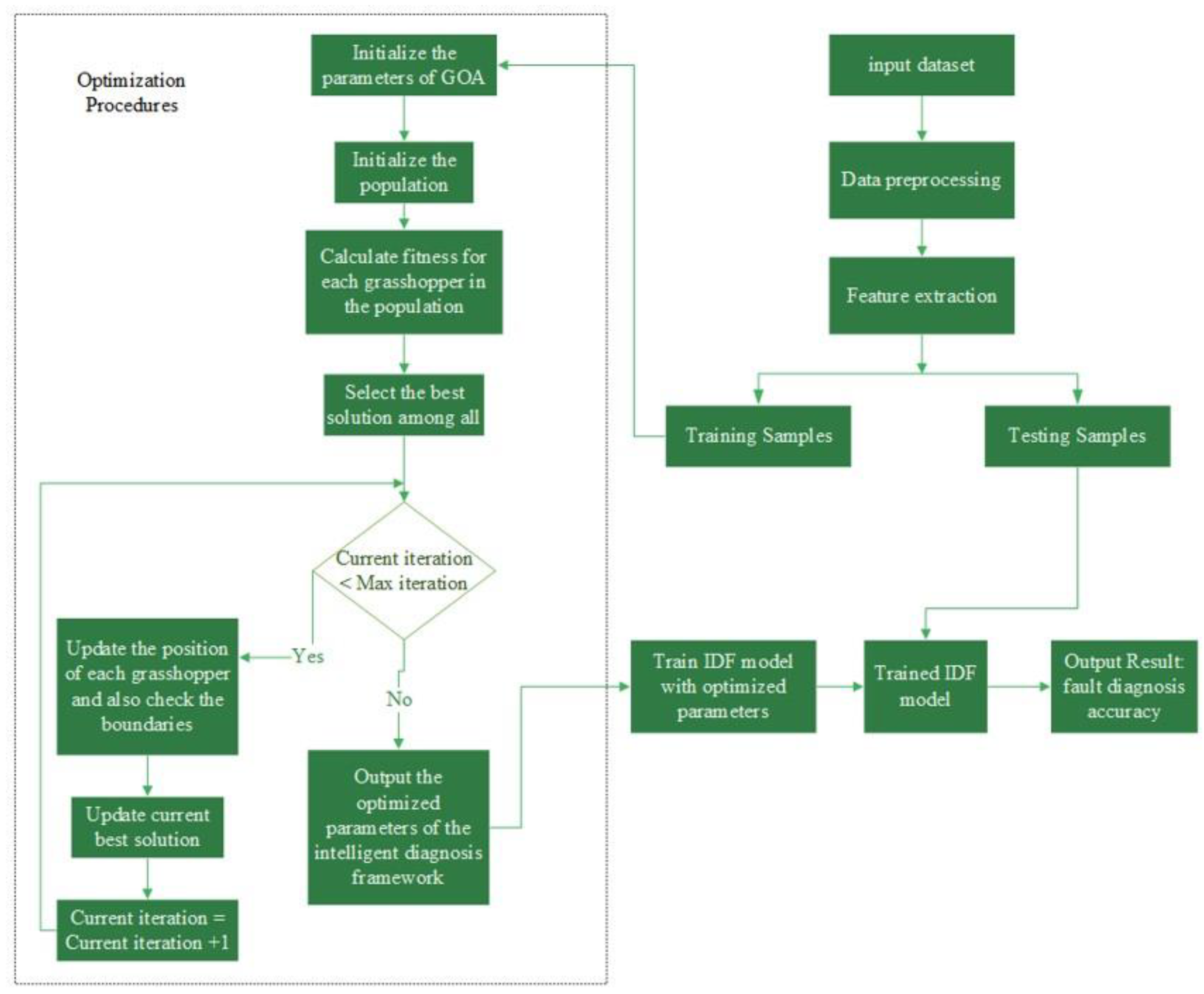
3.1. Proposed Intelligent Diagnosis Framework

The proposed Intelligent Diagnosis Framework (IDF) based on machine learning techniques is discussed here to classify the two distinctive units of observations into their relevant classes. It is a mathematical entity, a procedure for maximizing a specific mathematical characteristic about a set of data. The proposed framework is a supervised learning method that analyzes data for each classification and regression analysis. It can successfully handle high-dimensional and nonlinear records quite well. It offers a collection of instructions to forecast the necessary characteristics of unidentified checking-out data based on the structure of training statistics sets. The mechanism of the proposed framework is based on discovering the nice hyperplane that separates the records of two exceptional lessons of the category. The best hyperplane is the one that maximizes the margin or the separation between it and the closest coaching spots. The following is how the suggested framework’s structural design is supported: First, to manage the trade-off between margin maximization and a variety of misclassifications, the regularization parameter C is applied. Second, kernel characteristics for converting training data from a lower dimension’s characteristic space to a higher dimension’s characteristic space hyper-parameters refer to all kernel features, such as linear, polynomial, radial groundwork function, and sigmoid, that have certain free parameters. The kernel generally used in the research was the Gaussian or radial basis function (RBF) kernel with width σ, which is represented as

$$K(m,n)=\mathrm{e}\mathrm{x}\mathrm{p}(-||m-n||2/2\sigma 2)$$

(1)

Here, K(m,n) is termed the kernel function, which is founded on the dot product of two invariants, x and y. The suitable trade-off parameter C and the kernel parameter σ are required to educate the proposed framework classifier and are generally obtained using the capability of the K-fold cross-validation technique. The application of the proposed framework may provide two challenges: choosing the right kernel feature and modifying its parameters. Finding the optimum decision plane is a computational optimization challenge that helps kernel functions locate the appropriate space for linearly separating instructions using a nonlinear transformation.

The working process of the proposed intelligent framework of two different classes is mentioned in the following to classify them. For taking set A to train

$$A=\left\{mk , nk\right\}uk=1$$

(2)

where $m_k\mathsf{ϵ}{\mathbb{R}}^N$ and $n_k\mathsf{ϵ}\left\{-1,+1\right\}$. Now, the goal of the proposed framework is to assemble a most effective hyperplane in the following way:

$$g\left(m\right)=w^T{m}_k+b={\sum }_{p=1}^u{w}_p{m}_p+b=0$$

(3)

Here, the bias value, denoted by b, is a scalar and weight vector. The function of the isolating hyperplane is controlled by a vector $m_k\mathsf{ϵ}{\mathbb{R}}^N$ and scalar b. The signal g(m) is used to make a choice characteristic for producing a hyperplane that classifies the input records into either a superb or terrible class. Thus, the discrete distinguishing of hyperplanes has to fulfill the following requirements:

$$g\left(m_i\right)=+1 \mathrm{if}, n_i=+1$$

(4)

$$g\left(m_i\right)=-1 \mathrm{if}, n_i=-1$$

(5)

It can be stated as

$$n_{i}g\left(m_i\right)=n_i(w^T{m}_i+b)\ge 1 \mathrm{for} \mathrm{I} = 1,2,\dots , \mathrm{U}$$

(6)

By positioning and orienting a hyperplane between the two unique groups in this method, the margin can be increased while minimizing generalization error. Guide vectors are the fact points used to specify the margin that is closest to the hyperplane. A hyperplane that allows linear separation in higher dimensions can be created for this circumstance when linear separation may not be adequate to appropriately separate two classes. It is referred to as a linear aid vector machine if the data region can be split linearly (straight line or hyperplane) to distinguish the classes in the real domain. When the information domain cannot be divided linearly, nonlinear help vector machines can be used instead. These machines can be moved to a house known as the characteristic space, where the information domain can be divided linearly to separate the classes.

To distinguish data from distinct classes, the proposed framework calculates a maximum margin hyperplane. $m_i$ denotes the input vector; $n_i$ denotes the labels; L denotes the total number of samples; b denotes the dimension of the input vector:

$${\underset{\mathit{\omega },b,\xi }{\min }\frac{1}{2}‖{\omega }^{\prime }‖}^2+C {\sum }_{l=1}^L{\xi }_l$$

(7)

$$\begin{gathered} n_{l }\left[\left({\omega }^{\prime } . {m^{\prime }}_l\right)+b\right]-1+{\xi }_l \ge 0, l=1,2,\dots \dots ,L \\ {\xi }_{l }\ge \mathrm{0,1},\dots \dots ,L \end{gathered}$$

where ${\omega }^{\prime }$ is an n-dimensional vector, b denotes a scalar, C denotes a regularization parameter, and ${\xi }_l$ denotes the slack variable. For a nonlinear situation, the ideal hyperplane in the high-dimensional feature space can be formed as follows.

$${\underset{\mathit{\omega },b,\xi }{\min }\frac{1}{2}‖{\omega }^{\prime }‖}^2+C \sum _{l=1}^L{\xi }_l$$

(8)

$$\begin{gathered} { n}_{l }\left[\left({\omega }^{\prime } . {{\phi (m}^{\prime }}_l)\right)+b\right]-1+{\xi }_l \ge 0, l=1,2,\dots \dots ,L \\ { \xi }_{l }\ge \mathrm{0,1},\dots \dots ,L \end{gathered}$$

The decision function in the developed intelligent framework is specified as

$$f\left(x\left(t\right)\right)={\sum }_{i=1}^{M}K\left(x_i^{*},x\left(t\right)\right)+b^{*}$$

(9)

where $x_i^{*}$ is $i^{th}$ vector of M support vectors, $y_i$ is the class label, and x(t) is the $t^{th}$ input frame vector. The optimization bias b* and the Lagrange multiplier $\alpha$* may be derived by successfully resolving a quadratic programming problem.

The following formula is obtained when the radial basis function is used as the kernel function K(xi*, x(t)):

$$\mathrm{K}\left(\mathrm{x}\mathrm{i} \mathrm{*},\mathrm{x}\left(\mathrm{t}\right)\right)=\mathrm{e}\mathrm{x}\mathrm{p}\left(-\gamma {‖x_i^{*}-x\left(t\right)‖}^2\right)$$

(10)

where the RBF kernel parameter is denoted by γ. Algorithm 1 depicts the pseudo-code for the proposed framework.

In Algorithm 1, the variables Ni, Ns, and N_f denote the number of input vectors, support vectors, and features input and support vectors. The term sv[k] includes features for the proposed framework, and in[j] is a structure’s array containing an input vector’s feature array. Again, the variable m indicates K (xi*, x(t)) in Equation (11), and F indicates f(x(t)) in Equation (10). The outermost loop repeatedly delivers input vectors to the middle loop that is implemented in Equation (10), and the innermost loop computes the square of an input vector’s distance from a support vector.

Algorithm 1. Pseudo-code for the proposed intelligent framework.

1.  for i ← 1 to $N_i$ by 1 do 2.  F = 0 3.  for j ← 1 to $N_S$ by 1 do 4.  dist = 0 5.  for m ← 1 to $N_f$ by 1 do 6.  dist + = ${\left(\mathrm{s}\mathrm{v}\right[\mathrm{k}].\mathrm{f}\mathrm{e}\mathrm{a}\mathrm{t}\mathrm{u}\mathrm{r}\mathrm{e}[\mathrm{m}]-\mathrm{i}\mathrm{n}[\mathrm{j}].\mathrm{f}\mathrm{e}\mathrm{a}\mathrm{t}\mathrm{u}\mathrm{r}\mathrm{e}[\mathrm{m}\left]\right)}^2$ 7.  end 8.  $m=exp\left(-\gamma \times dist\right)$ 9.  F + = sv[k]. ${\alpha }^{*}\times m$ 10.  end 11.  F = F $+$ $b^{*}$ 12.  end

The proposed framework focuses on the regularization hyperparameter C, which is used to control the trade-off between increasing margins and reducing misclassification. Additionally, kernel features are used by way of nonlinear functions for mapping the datasets to greater dimensional characteristic spaces. However, this higher-dimension function house transformation wants much greater calculations. It is possible to observe a kernel method that controls this transformation, restricts the computation depth, and maintains the effects of higher-dimensional transformation.

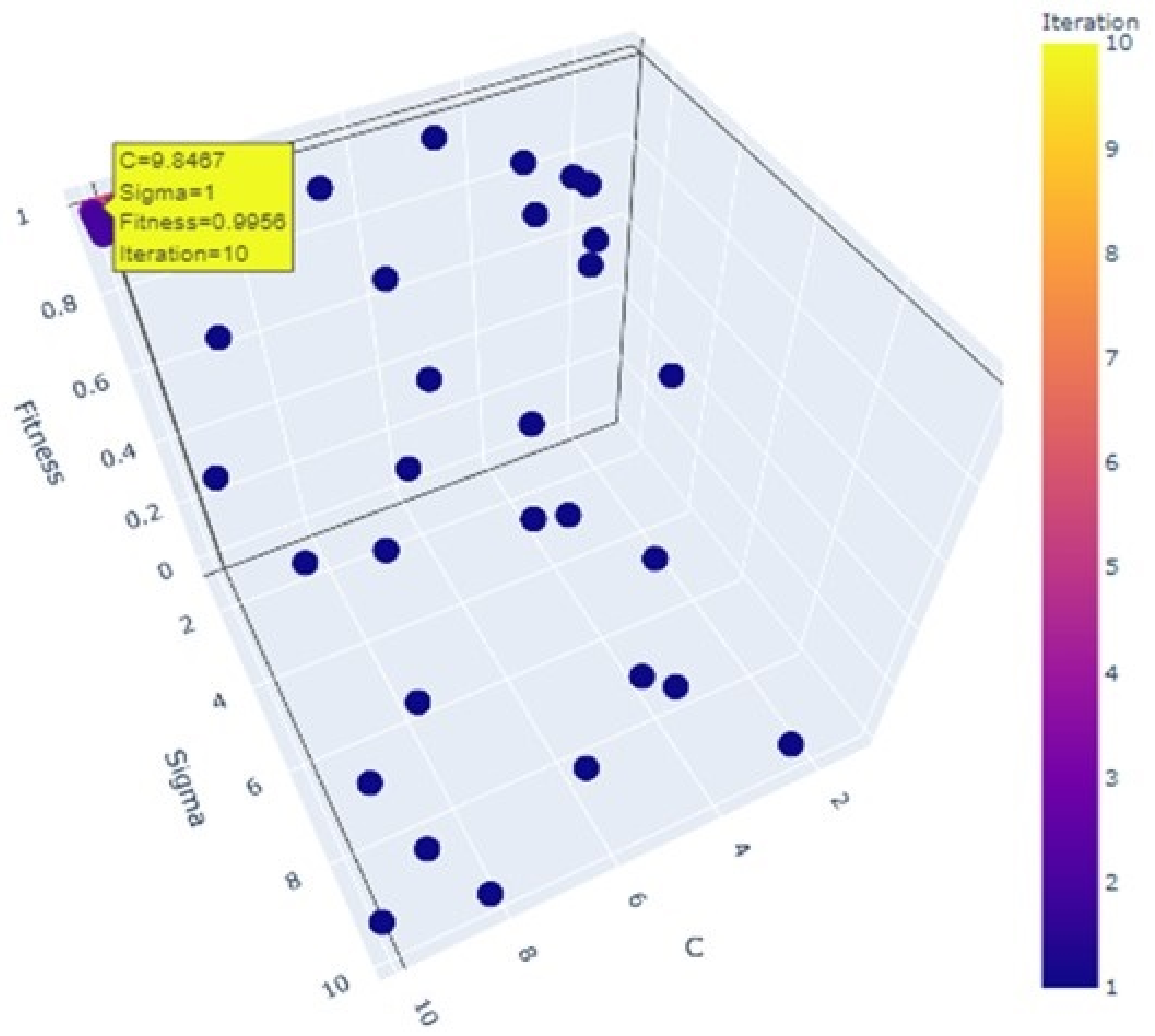
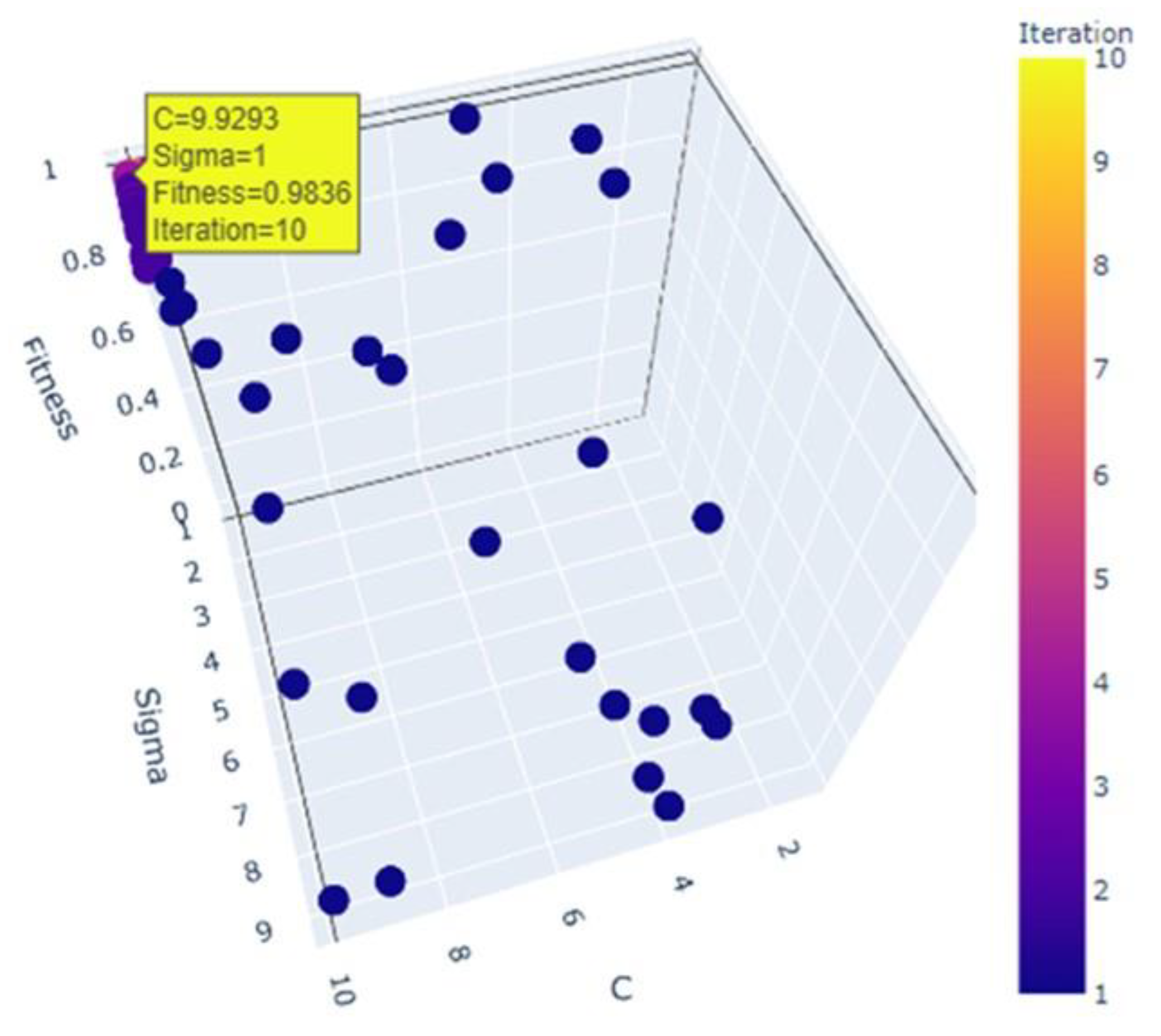
3.2. Design of Meta-Heuristic Optimization Algorithm

The Grasshopper Optimization Algorithm (GOA) stands out as an exceptional meta-heuristic optimization method, renowned for its accuracy and ease of application across a wide range of industrial scenarios. Meta-heuristic Optimization Algorithms have rapidly evolved and found applications in diverse fields, including signal detection, load balancing, feature resolution, and engineering processes. These algorithms share a common characteristic in their two primary phases: exploration and exploitation. In the exploration phase, they thoroughly investigate the search space, while the exploitation phase focuses on pinpointing optimal solutions within promising areas. For an effective meta-heuristic algorithm, striking a balance between exploration and exploitation is crucial. GOA draws inspiration from mature grasshoppers’ behavior, which involves both long-range and abrupt movements, reflecting the exploration phase, as well as nearby hops to seek better food sources, symbolizing the exploitation phase. What sets GOA apart is its ability to address shortcomings without placing significant emphasis on factors like the balance between exploration and exploitation or the relationship between population size and convergence speed during the optimization process.

A mathematical model for this conduct was introduced. The model is described as follows:

$${ x}_p=S_p+G+A$$

(11)

In this equation, x_p represents the p grasshopper’s function, S_p represents the group’s social interaction, G represents the gravitational effect acting on p, and A represents the direction of the wind. GOA analyzes only social interaction (S_p) to resolve optimization challenges.

$$S_p={\sum }_{\begin{array}{c}j=1\\ j\ne i\end{array}}^N s\left(d_{pq}\right)\widehat{d_{pq}}$$

(12)

where d_pq = |x_q − x_p| and $\widehat{{\mathrm{d}}_{\mathrm{p}\mathrm{q}}}$= $\frac{{\mathrm{x}}_{\mathrm{q}}-{\mathrm{x}}_{\mathrm{p}}}{{\mathrm{d}}_{\mathrm{p}\mathrm{q}}}$, and G component in Equation (1) is obtained as ${\mathrm{G}}_{\mathrm{p}}=-\mathrm{g}\widehat{{\mathrm{e}}_{\mathrm{g}}}$, component. Now, the term A in Equation (1) is determined as

$${\mathrm{A}}_{\mathrm{p}}=\mathrm{u}.\widehat{{\mathrm{e}}_{\mathrm{w}} }$$

(13)

Depending on where an individual grasshopper is relative to nearby grasshoppers, it may experience the three forces of attraction, repulsion, and neutrality in a grasshopper swarm. To demonstrate how grasshoppers interact in terms of comfort zone:

$$\mathrm{S}\left(\mathrm{r}\right)=\mathrm{f}{\mathrm{e}}^{-\frac{\mathrm{r}}{\mathrm{l}}}-{\mathrm{e}}^{-\mathrm{r}}$$

(14)

Here, f denotes the level of attraction, and l is the scale of attractive length. By expanding Sp, G and A in Equation (11) can be rewritten as follows:

$${\mathrm{X}}_{\mathrm{p}}={\sum }_{\mathrm{q}=1,\mathrm{j}\ne 1}^{\mathrm{N}}\mathrm{s}\left(\left|{\mathrm{x}}_{\mathrm{q}}-{\mathrm{x}}_{\mathrm{p}}\right|\right)\frac{{\mathrm{x}}_{\mathrm{q}}-{\mathrm{x}}_{\mathrm{p}}}{{\mathrm{d}}_{\mathrm{p}\mathrm{q}}} -\mathrm{g}\widehat{{\mathrm{e}}_{\mathrm{g}}}+\mathrm{u}\widehat{{\mathrm{e}}_{\mathrm{w}}}$$

(15)

To solve optimization problems effectively, a stochastic algorithm has to perform exploration and exploitation successfully, approximating the global optimum as accurately as possible. The GOA method uses the following mathematical model for grasshopper position updates:

$${\mathrm{X}}_{\mathrm{d}}^{\mathrm{p}}=\mathrm{c}({\sum }_{\mathrm{q}=1,\mathrm{j}\ne \mathrm{i}}^{\mathrm{N}}\mathrm{c}\frac{\mathrm{u}{\mathrm{b}}_{\mathrm{d}}-\mathrm{p}{\mathrm{b}}_{\mathrm{d}}}{2}\mathrm{S}\left(\left|{\mathrm{X}}_{\mathrm{q}}^{\mathrm{d}}-{\mathrm{X}}_{\mathrm{p}}^{\mathrm{d}}\right|\right)\frac{{\mathrm{x}}_{\mathrm{q}-}{\mathrm{x}}_{\mathrm{p}}}{{\mathrm{d}}_{\mathrm{p}\mathrm{q}}})+\widehat{{\mathrm{T}}_{\mathrm{d}}}$$

(16)

The coefficient c decreases the remedy area equivalent to the wide variety of generations:

$$\mathrm{c}={\mathrm{c}}_{\mathrm{m}\mathrm{a}\mathrm{x}}-\mathrm{iter} \frac{{\mathrm{c}}_{\mathrm{m}\mathrm{a}\mathrm{x}}-{\mathrm{c}}_{\mathrm{m}\mathrm{i}\mathrm{n}}}{\mathrm{M}\mathrm{a}{\mathrm{x}}_{\mathrm{i}\mathrm{t}\mathrm{e}\mathrm{r}}}$$

(17)

The optimization process is often divided into two stages, exploration and exploitation, and in each case, the teaching of nature-inspired algorithms emphasizes the importance of improving the probability up until a stop condition is reached. The Grasshopper Optimization Algorithm is a successful approach with many benefits, including simplicity in development, efficiency in searching, and ease in modifying algorithm parts.

Algorithm 2 depicts the GOA algorithm in pseudo-code form. To begin optimization, the GOA generates a list of possible solutions at random. The locations of the search agents are changed by using Equation (17).

Algorithm 2. Pseudo-codes of the Grasshopper Optimization Algorithm.

Start the swarm Xp(p = 1, 2,3, ....., n) Set up $c_{max}$, $c_{min}$, , and max no. of iterations Calculate each search agent’s fitness. L = the best search agent While (t < Limit of iterations) Adjust c with the aid of Equation (17) For each search agent    Standardize the spacing between agents [1,10]    Adjust the equation to reflect the changed location of the search agent (17)    If the search agent leaves the specified boundary, bring it back. end for Update L and position if a better solution is available. $t=t+1$  End While Return L (the target fitness and target position)

Every iteration maintains the position of the excellent target purchased in such a manner. Additionally, problem C is determined using Equation (17), and for each iteration, the separations between the grasshoppers are normalized in [1,10]. Position updates are performed repeatedly until a stop requirement is satisfied. The international optimum is eventually best approximated by the role and fitness of the first-class goal.

3.3. Meta-Heuristic Optimization Configured Intelligent Diagnosis Framework

The proposed MHOA-IDF model’s entire process is depicted schematically in Figure 1. The proposed method begins by importing the acquired data, as shown in the diagram. The preprocessing techniques, such as data preprocessing and missing value handling, are then performed. We will create a feature matrix later by utilizing the input dataset by computing time-domain features. The feature extraction divides huge quantities of raw data into smaller sections that can be processed further. The major purpose of this method is to select variables and convert them into features, therefore compressing the data that must be processed while correctly categorizing the main data set. A large amount of data is necessary to detect the fault precisely. As a result, feature extraction is important to the process’s simplification. From the time-domain data, ten features were extracted. Max, min, mean, standard deviation, skewness, kurtosis, root mean square, crest, and form factor are the time-domain characteristics obtained from the signal. Time-domain features for the feature matrix are shown in

Table 1. Comparison for bearing fault diagnosis published in previous years.

References	Accuracy	Classifier	Data Amount	Fault Type	Required Time	Efficient	Robustness (High)
[37]	97.27%	GAN	High	10	Moderate	Yes	Yes
[38]	90.28%	MPE-PSOSVM	High	6	High	Yes	Yes
[38]	96.56%	VMD-MPE-PSOSVM	Medium	6	High	Yes	Yes
[39]	89.2%	VMD and GMDE	Medium	4	High	No	Yes (Noise only)
[40]	97.09%	Triplet Network + SVM	High	9	Low	No	Yes
[1]	93.8	Quadratic SVM	High	4	High	Yes	No
[41]	99.77%	CNN + LSTM Network	High	5	High	Yes	No
[42]	98.5%	GWO-SVM	Medium	8	Low	No	No
[43]	98.24%	Hybrid CNN	High	3	High	No	No
Proposed	High	GOA-SVM	High	15	Low	Yes	Yes

.

The training and testing sections are then carried out using a cross-validation method. After that, MHOA is used to optimize proposed diagnosis framework parameters based on the training data. The MHOA algorithm is performed to obtain the optimal parameters.

To optimize the two parameters, c and σ, using the Meta-heuristic Optimization Algorithm (MHOA), the following process is employed:

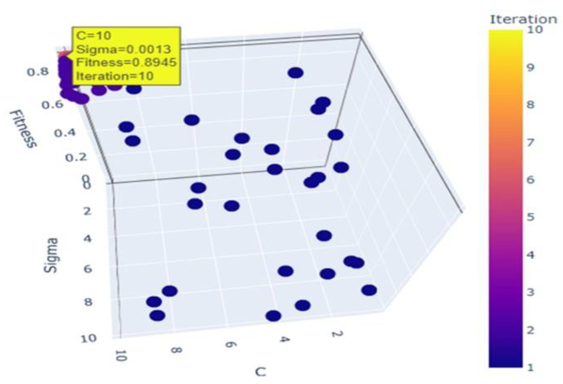
• Initialization: Set the parameters for the Grasshopper Optimization Algorithm (GOA). Here, we configure the maximum number of iterations to 10 and define a population size of n= 30 grasshoppers.
• Fitness Assessment: Evaluate the fitness of each grasshopper within the population and identify the best solution among them.
• Iteration Check: Check if the current iteration is within the defined maximum iteration limit. If it is, proceed to the next step (Step 4); if not, display the best solution found and conclude the process.
• Position Update: Update the positions of the grasshoppers while considering the distances between them. This step also involves checking if any grasshoppers have strayed beyond the defined boundaries.
• Best Solution Update: Update the current best solution and replace it with any new, superior solution that emerges during the iteration.
• Iteration Control: Increment the iteration counter and verify if the current iteration is still below the maximum iteration limit. If this condition holds true, return to Step 4 for the next iteration. If it is false, display the best solution obtained.
• Output: Finally, present the optimized parameters for the proposed Intelligent Diagnosis Framework.

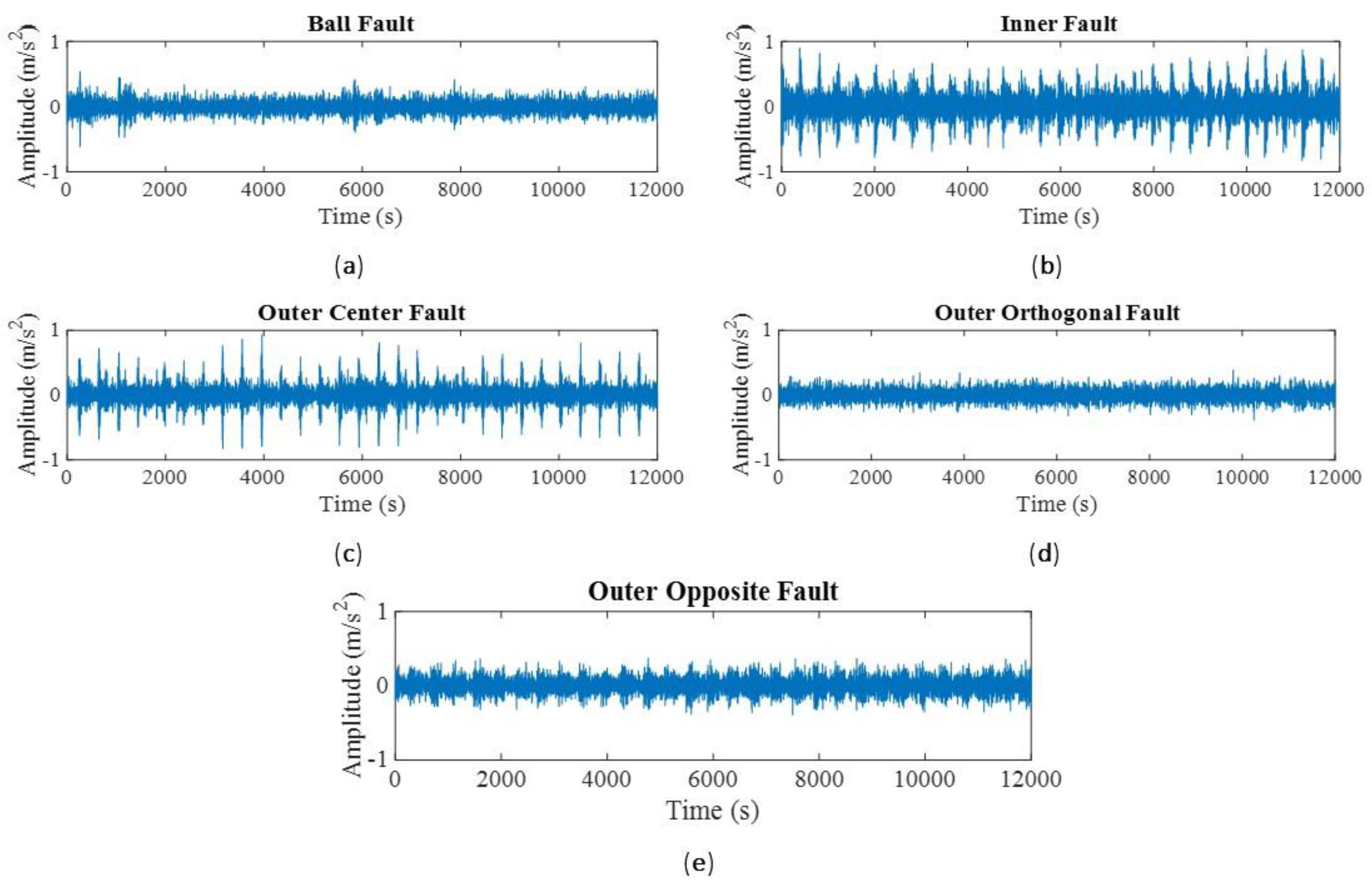
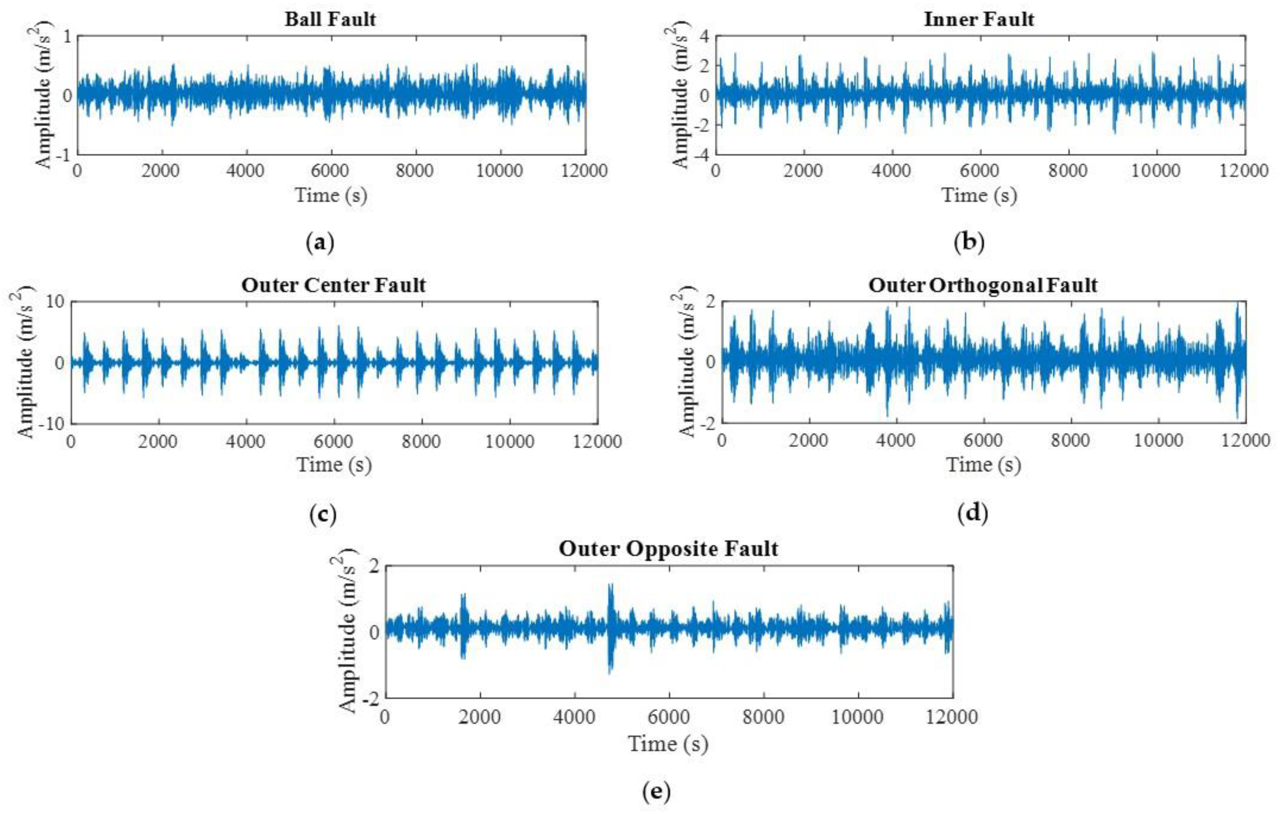
This section examines issues regarding the optimal and overall performance of the MHOA algorithm. The results are then furnished and analyzed in detail.

4. Dataset

The dataset for this experiment is collected from the Case Western Reserve University (CWRU) bearing dataset.

fault, and 12,000 fan end fault. Each category contains data sets for ball faults and inner and outer race faults. The outer race faults are split into three sections based on “centered” (a fault at 6 o’clock), “orthogonal” (3 o’clock), and “opposite” (12 o’clock). Some features and description of the dataset are as follows:

Data Type: The CWRU bearing fault dataset contains vibration data collected from accelerometers placed on a test rig that simulates a rotating machinery system. The data are collected in the form of time-domain and frequency-domain signals.

Bearing Types: The dataset includes data from two types of bearings:

• Ball Bearings;
• Roller Bearings.
• Fault Types: There are several fault conditions simulated in the dataset:
• Normal (healthy) condition;
• Inner race fault (IR);
• Outer race fault (OR);
• Ball fault (BF);
• Cage fault (CF).

Data Size: The dataset is organized into multiple files, each containing data for different combinations of bearing types and fault conditions. The dataset is relatively large, with each file containing thousands of data points. In total, the dataset contains tens of thousands of data points.

Data Characteristics: The data are collected at varying motor load conditions, which make them more representative of real-world scenarios where machinery operates under different loads. The sampling frequency for the data is typically 12 kHz, although there may be variations in different subsets of the dataset.

Data Format: Each data file is typically in a text format with columns for time and vibration measurements. These measurements are taken at different positions on the test rig, and the columns correspond to different sensor locations.

The pressure motor is put to the test, and the analog defect is detected with the help of an accelerometer attached to the motor’s driving end. The signal’s data are sampled at a rate of 12,000 per second. Figure 2 illustrates the experimental setup for rolling bearings. Acceleration data were collected from the motor bearings during testing using a 2 hp Reliance Electric motor. A two-horsepower Reliance Electric motor operates a shaft that holds a torque transducer and an encoder. To apply torque to the shaft, a dynamometer and an electronic control system are used. Bearings were contaminated with faults utilizing an electro-discharge machining (EDM) process. Inner raceway, ball, and outer raceway faults were inserted in a certain order, with fault dimensions ranging from 0.007 to 0.040 inches (0.18 to 0.71 mm). After replacing the faulty bearings in the test motor, vibration measurements were taken at loads from 0 to 3 horsepower (motor speeds of 1797 to 1720 RPM). A summary of the variation of parameters over the generation is shown in

Table 2. Diameter and load condition for various fault level generation.

Bearing Status	Diameter (in)	Motor (hp)	Label
Ball fault	0.007	0, 1, 2, 3	BF
	0.014
	0.021
	0.028
Inner race fault	0.007	0, 1, 2, 3	IF
	0.014
	0.021
	0.028
Outer fault centered load zone	0.007	0, 1, 2, 3	OFC
	0.014
	0.021
Outer fault orthogonal load zone	0.007	0, 1, 2, 3	OFO
	0.014
	0.021
Outer fault opposite load zone	0.007	0, 1, 2, 3	OFOP
	0.014
	0.021

. Acceleration was observed on the base (BA), the fan end bearing, and the drive end bearing during each test. Four distinct groups of data are distinguished by their sample rate (12 or 48 kHz) and the position of the faulty bearing: 48,000 baseline, 12,000 drive end fault, 48,000 drive end fault, and 12,000 fan end fault.

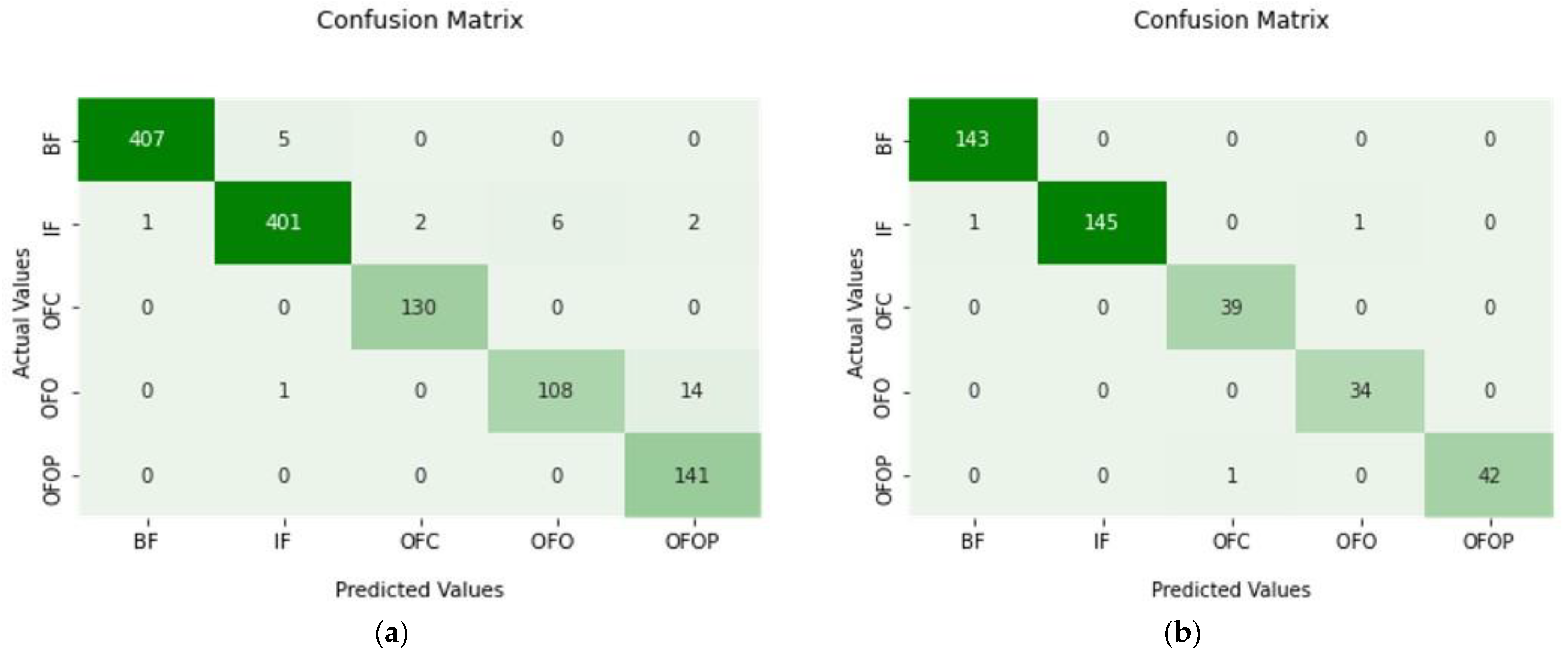
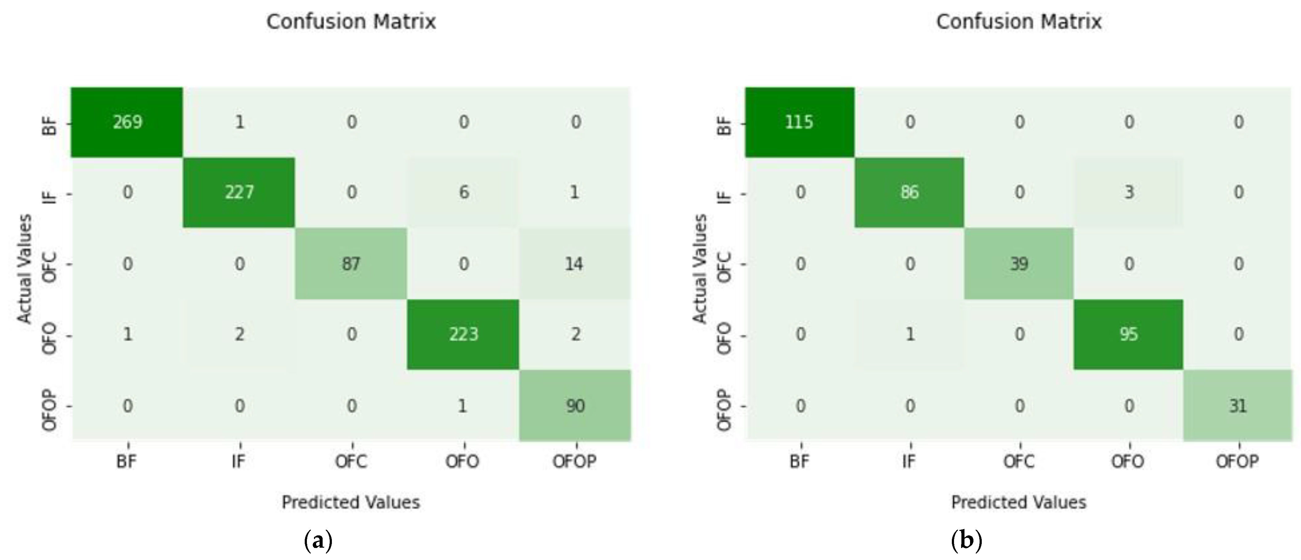
5. Experimental Results

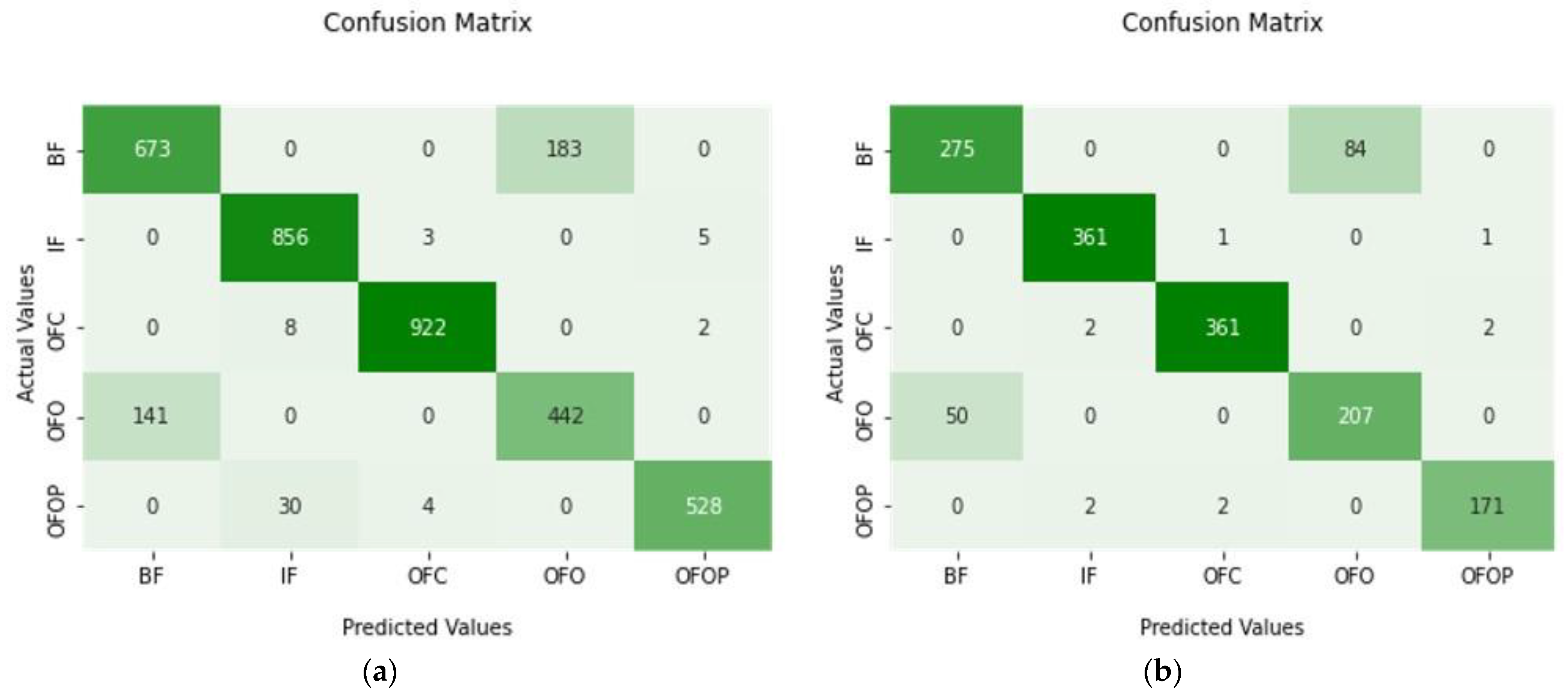
Frequency-related data are significant in the vibration study of the bearings, but feature extraction becomes extremely important in the auto fault detection system. Using Python programming, the attributes shown in

Table 3. Time-domain features for the feature matrix.

Feature	Equation	Feature	Equation
Mean:	$\mu =\frac{1}{N} {\displaystyle \sum _{i-1}^N}{x}_i$	RMS:	$X_{rms}=\sqrt{\frac{{\sum }_{i=1}^N{x_i}^2}{N}}$
Standard Deviation:	$\sigma =\sqrt{\frac{\sum _{i=1}^N{\left(x_i-\mu \right)}^2}{N-1}}$	Crest factor:	$C_f=\frac{X_{max}}{X_{rms}}$
Skewness:	$x_{skewness }$= $\frac{1}{N}\frac{\sum _{i=1}^N{\left(x_i-\mu \right)}^3}{{\sigma }^3}$	Form factor:	$F_f$ $=\frac{{Xrms}_{}}{\mu }$
Kurtosis:	$x_{kurtosis }=$ $\frac{1}{N}\frac{\sum _{i=1}^N{\left(x_i-\mu \right)}^4}{{\sigma }^4}$

were retrieved from all the signals: maximum, minimum, mean, kurtosis of the signal, standard deviation, skewness, root mean square, crest factor, and form factor value. The results of employing MHOA-IDF to identify and categorize bearing faults are shown in this section. The dataset is used to train the MHOA-IDF algorithm in this regard. The enormous amount of data and the usage of IDF are responsible for the subpar classification results. The only way to resolve this problem is to combine MHOA with IDF. We divided the dataset into segments to extract features. We used the appropriate formulae for each segment to determine the value. Three cases make up the whole dataset. Each case contains one of five fault kinds. The effectiveness of various model types, the setup of settings, and the preparation of datasets are all covered in great detail in this section. The proposed MHOA-IDF fault diagnosis method is applied in three cases to evaluate the method and confirm its suitability for locating rolling bearing defects. This research runs three tests for each of the five defects to further verify the stability of the approach, and the results of the classification are shown below.

5.1. Case 1

The CWRU bearing dataset, which is accessible on the CWRU bearing website, was used in this investigation. We utilized the 12,000 drive end fault data for the experiment in case 1. Figure 3 displays the time-domain waveform for each fault for the 12,000 drive end data of the vibration signals of the bearings in various states for each of the five types of faults that we use.

Each of them was plotted on a MATLAB simulation. Each represents different states of the time-domain waveform for case 1. The test rig’s drive-end bearing, which has a variety of defects, provided the vibration data at a sampling frequency of 12,000 Hz used in this research. In this experiment, we generated five distinct statuses, each with four distinct load scenarios, for the failed bearing signals. Ball fault, inner race fault, outer centered fault, outer orthogonal fault, and outer opposite fault are all used with motor loads between 0 and 3 horsepower.

The 12,000 drive end-bearing dataset must first be mined for vibration signals. We may compute time-domain features on the full signal or on subsets of it to obtain the feature matrix. Seven integers will result from computing seven features on the full signal. A better approach is to divide the raw data into 1410 b segments that do not overlap one another. Each time-domain feature is computed for a length of 1410 segments. The time-domain properties of each signal may be calculated using the formulae presented in Table 3. At least 80% of the bearing samples are randomly chosen for training, while the other 20% are utilized for testing. Optimize the IDF parameters using GOA using the samples that were chosen at random. The final optimization results are best: C = 9.8467, best σ = 1, and best fitness = 0.9956.

To train the IDF model and generate a trained IDF model, the optimal parameters shown in Figure 4 should be employed. Then, enter the test samples into the IDF model, train it, and use it to categorize and identify the test dataset. The diagnostic precision of the proposed method is 99.26% measured using the confusion matrix shown in Figure 5. The diagnostic precision using IDFs is 97.45%. The comparison demonstrates the importance of MHOA in maximizing IDF parameters.

5.2. Case 2

From the same CWRU bearing dataset, 12,000 fan end fault data have been used for case 2. Similarly, the test rig’s fan end bearing supplied the vibration data for this study at a sampling frequency of 12,000 Hz shown in Figure 6. The five fault types are similar to the previous case 1 for a motor load of 0–3 hp.

For case 2, time-domain waveforms for the five fault categories that we use are shown in Figure 7 for the 12,000 fan end data of the vibration signals from the bearings at various states. A MATLAB simulation graph was used to depict each. There are many different states that a waveform can be in during its passage through time.

Comparable to case 1 from before, the data preparation method was similar. To produce the feature matrix, time-domain features must be calculated for either the whole signal or a subset of it. Calculating seven characteristics throughout the whole signal yields seven digits. A more effective strategy is to divide the raw data into 1410 non-overlapping pieces of the same length. Each time-domain feature is computed for a length of 1410 segments. We randomly choose at least 80% of all bearing samples for training and utilize the remaining 20% for testing. Apply MHOA to optimize the IDF parameters using the randomly sampled data. The final optimization results are best C = 9.9293, best σ = 1, and best fitness = 0.9836. Using the best parameters, a trained IDF model was developed. The proposed technique accurately identifies and categorizes the test dataset using a MHOA-IDF model and gives 98.92% accuracy measured by using the confusion matrix shown in Figure 8.

The accuracy of IDF diagnosis is 96%. MHOA improves IDF parameters comparatively.

5.3. Robustness Measurement (Case 3)

In case 3, we used the 48,000 drive end fault data for the experiment. The vibration signals employed in this study originated from the faulty drive end bearing of the test rig as shown in Figure 9. The sampling frequency was 48,000 Hz. For a motor load of 0–3 hp, the types of faults used are the same as before: ball fault, inner race fault, outer centered fault, outer orthogonal fault, and outer opposite fault.

For the five fault categories we employ, for the 48,000 drive end data of the vibration signals from the bearings in their various states. A graphical representation of a MATLAB simulation was used to depict each. Different stages of a waveform’s evolution are possible at any given instant.

Finally, case 3 is illustrated in Figure 9, which displays the time-domain waveforms for the five fault categories we employ for the 48,000 drive end data of the vibration signals from the bearings in their various states. A graphical representation of a MATLAB simulation was used to depict each. Different stages of a waveform’s evolution are possible at any given instant.

The feature matrix is generated by computing time-domain features on all or a portion of the signal. Seven numbers are the result of calculating seven features throughout the whole signal. To obtain the most out of the data, it is best to cut it into 1410 uniformly sized parts that do not overlap. A total of 1410 segments are used in the computation of each time-domain characteristic. During training, we use at least 80% of all available bearing samples, while the remaining 20% are put to use during testing. Use MHOA to fine-tune the IDF settings based on the randomized data. One IDF model was trained using the optimal settings shown in Figure 10. Accuracy in diagnosis is 90.58% using the recommended strategy measure from Figure 11. IDFs have an accuracy of 89.9% in diagnostics. The results show that MHOA is crucial for optimizing IDF settings.

The confusion matrix shows the total signals examined and how many were correctly categorized. The confusion matrix, overall accuracy, recall, precision, and the F1-score are the performance measures in this research. The assessment parameters are established using the equations shown in

Table 4. Performance evaluation parameters.

Accuracy = $\frac{TP+TN}{TP+FP+TN+FN}$

Precision = $\frac{TP}{TP+FP}$

Recall = $\frac{TP}{TP+FN}$

F1 score = $2\times \frac{Precision\times Recall}{Precision+Recall}$

.

The output of the MHOA-IDF model based on the performance measures is shown in

Table 5. Results of the MHOA-IDF in terms of the evaluation parameters.

Data	Accuracy	Precision	Recall	F1 score
12,000 drive end	99.26%	98.79%	99.26%	99.02%
12,000 fan end	98.92%	99.15%	99.1%	99.13%
48,000 drive end	90.58%	90.53%	88.98%	88.85%

. The MHOA-IDF approach was successful in three instances. For three cases, the output has been shown. From case 1, 12,000 drive end data have the most accuracy, then comes 12,000 fan end data from case 2, and lastly, case 3, 48,000 drive end data. All these parameters are calculated explicitly.

With 12,000 drive-end data, Figure 12 shows that the fitness is marginally below 0.994 for the first iteration. For 12,000 fan end data, the minimum fitness level is 0.9804, whereas for 48,000 drive end data, it is 0.887. Iterations after that have a little greater fitness value than the minimum. The system has rather strong robustness and interference-fighting capabilities after classifying them with MHOA. The 12,000 drive end-bearing dataset produces superior results compared to the other examples. Classification accuracy for the proposed MHOA-IDF was 99.26%.

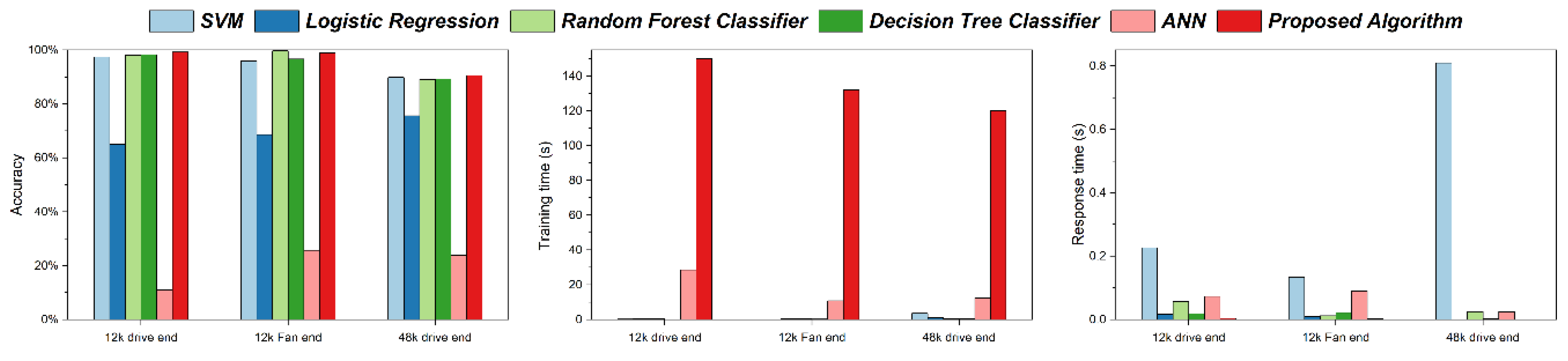
5.4. Comparative Analysis

We have provided a comparison, as shown in

Table 6. Comparison with other machine learning algorithms.

Dataset	12,000 Drive End			12,000 Fan End			48,000 Drive End
Model	Accuracy	Training Time (s)	Response Time (s)	Accuracy	Training Time (s)	Response Time (s)	Accuracy	Training Time (s)	Response Time (s)
SVM	97.45%	0.21	0.227	96%	0.16	0.133	89.9%	3.55	0.81
Logistic Regression	65.02%	0.58	0.017	68.64%	0.59	0.009	75.64%	1.14	0.0003
Random Forest Classifier	98.05%	0.61	0.057	99.72%	0.43	0.012	89.15%	0.48	0.025
Decision Tree Classifier	98.26%	0.20	0.019	96.72%	0.22	0.022	89.38%	0.62	0.003
ANN	11.06%	28.67	0.073	25.68%	10.82	0.09	23.80%	12.4	0.024
Proposed Algorithm	99.26%	150.05	0.004	98.92%	132.04	0.002	90.58%	120	0.0002

and Figure 13, between our proposed MHOA-IDF and other related machine learning algorithms. The comparison is based on our dataset, the CWRU bearing datasets, for three cases on the accuracy, training time, and average reaction time parameters. The comparison parameters are measured by using the same configuration computer, and it may change according to the computer configuration. By observing the recorded performance, it can be stated that the proposed method, developed by MHOA-IDF, outperforms competing methods in terms of having less computational complexity. Here, the computational complexity mainly indicates achieving high accuracy with a lower response time. The obtained parameters from the comparison using three different datasets are reported in Table 6 and

Table 7. Comparison with other latest works.

Study Ref	Year	Method	12,000 Drive End	12,000 Fan End	48,000 Drive End	Database	Result
[13]	2022	Wavelet packet transform and convolutional neural network	X	X	X	Case Western Reserve University	97% Accuracy
[15]	2020	Discrete wavelet transform (DWT) + Random forest (RF) and Extreme gradient boosting (XGBoost)	X	X	X	Real-time dataset of machine	99% Accuracy
[33]	2023	Fault-tolerant control (FTC)	X	X	X	Real-time dataset of machine	Complexity reduction of 23.5%
[34]	2023	Adaptive synchronous demodulation transform (ASDT)	X	X	X	Real-time dataset of machine	Mean error = 0.0237
Our work	Proposed	Grasshopper Optimization Algorithm with Improved Dimensional Filtering	✔	✔	✔	Public datasets	Accuracy = 90%

. It can be noticed that a considerable amount of training time is required for the proposed intelligent framework as it integrates a meta-heuristic optimization approach with the ML framework, which generally demands large processing power. Although the proposed framework takes a long time to train itself, it can provide improved accuracy, as well as reduce response time over the change of system parameters variation. This is possible because of its ability to reach a global optimum solution for the given optimal problem. Finally, it can be concluded that the proposed method provides low computational complexity in bearing fault diagnosis, as the efficacy of any intelligent framework relies on its response time and level of accuracy. In both cases, the proposed method confirms high effectiveness as compared to other related approaches.

High sampling frequency data often introduce additional noise, making accurate analysis a challenge, especially in real-world scenarios. The proposed GOA-IDF (Grasshopper Optimization Algorithm with Improved Dimensional Filtering) offers a solution by integrating the Improved Dimensional Filtering (IDF) technique. IDF effectively filters out noise and irrelevant data components, emphasizing critical features. The GOA component of the algorithm provides global optimization, aiding in the identification of robust patterns amidst the noise. This adaptability and noise-tolerant approach make GOA-IDF robust in real-world situations where data can be noisy and dynamic. Its ability to handle and mitigate noise while maintaining efficiency and accuracy is a significant advantage in applications such as predictive maintenance and fault diagnosis, where data quality can vary widely.

In the provided comparison using the CWRU bearing datasets, the newly proposed MHOA-IDF method is evaluated against other machine learning algorithms, considering accuracy, training time, and average reaction time parameters. The results indicate that the MHOA-IDF outperforms its competitors by achieving high accuracy with lower response times, demonstrating its computational efficiency. While it requires a relatively long training time due to its integration of meta-heuristic optimization and machine learning, it compensates with improved accuracy and reduced response times across varying system parameters. This efficiency is attributed to its ability to find global optimal solutions for complex problems. In conclusion, the MHOA-IDF method exhibits low computational complexity in bearing fault diagnosis, emphasizing the importance of response time and accuracy, and it proves highly effective compared to other related approaches in both aspects. Wang et al. [45] introduce a hybrid fault diagnosis method (WKN-BiLSTM-AM) that combines WaveletKernelNetwork and BiLSTM with an attention mechanism for improved bearing fault diagnosis accuracy, validated on multiple datasets, which is a similar approach, then our method. Accurate diagnosis of rolling bearing defects in electrical machinery presents a longstanding challenge, given their wide-ranging applications in energy and IoT manufacturing. The introduction of innovative electric motor designs often introduces new challenges, particularly in the form of rolling bearing faults. Precisely categorizing these bearing faults is essential for the efficient operation of motors in various industries. While numerous machine learning algorithms have been developed for fault characterization and condition estimation, their effectiveness is sometimes impeded by high computational costs and suboptimal hyperparameter selection. To address these challenges, this paper introduces an Intelligent Diagnosis Framework (IDF). However, the accuracy of IDF can be compromised due to limited datasets and suboptimal hyperparameters. Therefore, the paper suggests integrating the Grasshopper Optimization Algorithm (GOA), a meta-heuristic swarm intelligence optimizer, to enhance the performance of IDF. The effectiveness of the optimized GOA-IDF is evaluated using experimental data from Case Western Reserve University (CWRU), specifically the 12,000 drive end and 12,000 fan end datasets, in comparison with the non-optimized IDF. Furthermore, the paper conducts a comparative study with other machine learning algorithms to demonstrate the superior performance of the developed IoT GOA-IDF. Additionally, the paper investigates the robustness of GOA-IDF in handling high-frequency data, which may contain extraneous noise. The experiments conducted in this research underscore the competitive performance of the proposed GOA-IDF without compromising computational efficiency. Clarification: The paper’s focus is on the diagnosis of defects in rolling bearings, and it is crucial to highlight this distinction for clarity. Future studies can be based on using the latest techniques [3,46,47,48,49,50,51,52,53,54,55,56,57,58,59,60,61,62,63,64] that are based on innovative methods.

This study focuses on the importance of precise bearing fault diagnosis in rotating machinery, particularly in the context of industrial applications. Here are the summarized findings and key points:

• Importance of Bearing Fault Diagnosis: Bearing faults in rotating machinery can have significant consequences, leading to uncontrolled speed and potential damage to the entire system. The early monitoring and diagnosis of bearing conditions are crucial to prevent these issues.
• Data-Driven Techniques: The use of data-driven techniques for bearing fault diagnosis has gained popularity. These techniques are independent of system dynamics and can effectively classify and estimate faults based on recorded data.
• Support Vector Machine (SVM): SVM is highlighted as a top-of-the-line algorithm in machine learning for bearing fault diagnosis. However, incorrect parameter settings or kernel functions can lead to errors in fault detection.
• Optimization of SVM Parameters: Some studies have focused on optimizing SVM parameters for more accurate fault diagnosis. While heuristic methods can improve classification accuracy, they may be time-consuming and struggle to find the global optimal solution.
• Meta-Heuristic Optimization: To address the limitations of heuristic methods, the paper proposes a meta-heuristic configured intelligent framework for improving the accuracy of bearing fault diagnosis. It combines the Grasshopper Optimization Algorithm (GOA) and SVM.
• GOA: GOA is introduced as a bio-inspired optimization technique that balances global exploration and local exploitation in a high-dimensional search space. It is used for hyperparameter optimization in the proposed framework.

Heuristic Algorithms: The application of heuristic algorithms in combination with machine learning and deep learning approaches is discussed as a means to address optimization challenges.

The practical implications of this study are significant, particularly for industries relying on electrical machinery. The proposed Intelligent Diagnosis Framework (IDF) enhanced by the Grasshopper Optimization Algorithm (GOA) offers an efficient and accurate solution for diagnosing bearing defects, thereby ensuring the safety and reliability of electrical machinery. By addressing the challenges of high computational costs and suboptimal hyperparameter selection, this approach allows for more cost-effective and precise maintenance practices. The robustness of GOA-IDF in handling high-frequency data, even in the presence of noise, makes it a valuable tool for real-world applications, such as predictive maintenance in the energy and IoT manufacturing sectors. This study’s outcomes have practical relevance in improving the operational efficiency and safety of electrical machinery in various industries.

Future work in the field of the accurate diagnosis of bearing defects in electrical machinery could focus on the following areas:

• Enhanced Data Collection: Expand the dataset used for testing and training the diagnosis framework. Collect data from a wider range of operating conditions, motor types, and fault severities to improve the model’s generalization capabilities [46,47,48,49,50].
• Robustness to Real-World Conditions: Investigate the model’s performance in real-world industrial environments, where factors like varying loads, temperature fluctuations, and environmental noise can affect the accuracy of diagnosis. Developing techniques to make the model more robust to such conditions is essential [51,52,53,54,55].
• Online Monitoring and Predictive Maintenance: Develop methodologies for real-time monitoring and predictive maintenance. This would involve implementing the diagnosis framework on IoT devices or edge computing platforms for continuous monitoring and early fault prediction [3,56,57,58,59,60,61,62,63,64].
• Human–Machine Collaboration: Explore ways to integrate the diagnosis framework into human–machine collaboration systems. This could involve developing user-friendly interfaces that provide actionable insights to maintenance personnel, enabling them to make informed decisions [4,5,6,7,8].
• Integration with Maintenance Scheduling: Integrate the diagnosis framework with maintenance scheduling systems. This would enable the automatic scheduling of maintenance tasks based on the severity and urgency of detected faults.
• Fault Severity Estimation: Develop methods to estimate the severity of bearing faults accurately. Knowing the extent of a fault’s progression can help prioritize maintenance efforts and resources.
• Advanced Optimization Algorithms: Continue exploring and experimenting with different optimization algorithms beyond the Grasshopper Optimization Algorithm to further enhance the performance and efficiency of the diagnosis framework.
• Integration with Existing Systems: Develop strategies for integrating the diagnosis framework with existing industrial control and monitoring systems seamlessly [32,33,34,35,36,65,66,67].

6. Conclusions

In this research, we introduced a novel approach for classifying bearing defects, which combines the power of the Meta-heuristic Optimization Algorithm (MHOA) with the Intelligent Diagnosis Framework (IDF). The foundation of our approach lies in the extraction of essential features from the CWRU bearing dataset, which was meticulously prepared for fault diagnosis. We focused our attention on three distinct cases within the bearing dataset to thoroughly evaluate our methodology. Our approach can be divided into two primary stages. First, we harnessed the capabilities of the IDF machine learning algorithm to effectively categorize bearing faults. Subsequently, we addressed the critical issue of fine-tuning the IDF parameters using the optimization prowess of MHOA. This hybrid MHOA-IDF approach significantly boosts global search capabilities. In comparison to traditional methods such as IDF, Logistic Regression, Random Forest Classifier, Decision Tree Classifier, and Artificial Neural Networks (ANN), our approach stands out for its remarkable feature extraction capabilities and high accuracy. The empirical results from our experiments validate the effectiveness and robustness of our combined system, particularly when classifying faults under diverse noise conditions and varying motor load scenarios. It is worth noting that while our model demonstrates impressive performance, it does not demand excessive computational resources for data processing. However, it is essential to acknowledge that training the model without optimization can be time-consuming. As a potential avenue for future research, we encourage further investigations to enhance training efficiency by incorporating advanced mechanisms. In conclusion, our research presents a cutting-edge approach to bearing defect classification, offering an effective blend of feature extraction and parameter optimization. This method exhibits promise in real-world applications and contributes to the advancement of fault diagnosis in electrical machinery.

References

1. Parmar, U.; Pandya, D. Experimental investigation of cylindrical bearing fault diagnosis with SVM. Mater. Today Proc. 2021, 44, 1286–1290. [Google Scholar] [CrossRef]
2. Senanayaka, J.S.L.; Kandukuri, S.T.; Van Khang, H.; Robbersmyr, K.G. Early detection and classification of bearing faults using support vector machine algorithm. In Proceedings of the 2017 IEEE Workshop on Electrical Machines Design, Control and Diagnosis (WEMDCD), Nottingham, UK, 20–21 April 2017. [Google Scholar]
3. Wang, H.; Wu, X.; Zheng, X.; Yuan, X. Model Predictive Current Control of Nine-Phase Open-End Winding PMSMs With an Online Virtual Vector Synthesis Strategy. IEEE Trans. Ind. Electron. 2022, 70, 2199–2208. [Google Scholar] [CrossRef]
4. Ding, Z.; Wu, X.; Chen, C.; Yuan, X. Magnetic Field Analysis of Surface-Mounted Permanent Magnet Motors Based on an Improved Conformal Mapping Method. IEEE Trans. Ind. Appl. 2023, 59, 1689–1698. [Google Scholar] [CrossRef]
5. Liu, S.; Liu, C. Virtual-Vector-Based Robust Predictive Current Control for Dual Three-Phase PMSM. IEEE Trans. Ind. Electron. 2021, 68, 2048–2058. [Google Scholar] [CrossRef]
6. Liu, S.; Liu, C. Direct Harmonic Current Control Scheme for Dual Three-Phase PMSM Drive System. IEEE Trans. Power Electron. 2021, 36, 11647–11657. [Google Scholar] [CrossRef]
7. Liao, K.; Lu, D.; Wang, M.; Yang, J. A Low-Pass Virtual Filter for Output Power Smoothing of Wind Energy Conversion Systems. IEEE Trans. Ind. Electron. 2022, 69, 12874–12885. [Google Scholar] [CrossRef]
8. Li, J.; Deng, Y.; Sun, W.; Li, W.; Li, R.; Li, Q.; Liu, Z. Resource Orchestration of Cloud-Edge–based Smart Grid Fault Detection. ACM Trans. Sens. Netw. 2022, 18, 46. [Google Scholar] [CrossRef]
9. Aminizadeh, S.; Heidari, A.; Toumaj, S.; Darbandi, M.; Navimipour, N.J.; Rezaei, M.; Talebi, S.; Azad, P.; Unal, M. The applications of machine learning techniques in medical data processing based on distributed computing and the Internet of Things. Comput. Methods Programs Biomed. 2023, 241, 107745. [Google Scholar] [CrossRef]
10. Wang, L. (Ed.) Support Vector Machines: Theory and Applications; Springer Science & Business Media: Berlin/Heidelberg, Germany, 2005; Volume 177. [Google Scholar]
11. Saremi, S.; Mirjalili, S.; Lewis, A. Grasshopper Optimisation Algorithm: Theory and application. Adv. Eng. Softw. 2017, 105, 30–47. [Google Scholar] [CrossRef]
12. Abualigah, L.; Diabat, A. A comprehensive survey of the Grasshopper optimization algorithm: Results, variants, and applications. Neural Comput. Appl. 2020, 32, 15533–15556. [Google Scholar] [CrossRef]
13. He, F.; Ye, Q. A Bearing Fault Diagnosis Method Based on Wavelet Packet Transform and Convolutional Neural Network Optimized by Simulated Annealing Algorithm. Sensors 2022, 22, 1410. [Google Scholar] [CrossRef]
14. Zhu, J.; Hu, T.; Jiang, B.; Yang, X. Intelligent bearing fault diagnosis using PCA–DBN framework. Neural Comput. Appl. 2019, 32, 10773–10781. [Google Scholar] [CrossRef]
15. Toma, R.N.; Kim, J.-M. Bearing Fault Classification of Induction Motors Using Discrete Wavelet Transform and Ensemble Machine Learning Algorithms. Appl. Sci. 2020, 10, 5251. [Google Scholar] [CrossRef]
16. Amiri, Z.; Heidari, A.; Navimipour, N.J.; Unal, M.; Mousavi, A. Adventures in data analysis: A systematic review of Deep Learning techniques for pattern recognition in cyber-physical-social systems. Multimed. Tools Appl. 2023, 1–65. [Google Scholar] [CrossRef]
17. Guo, J.; Wan, J.-L.; Yang, Y.; Dai, L.; Tang, A.; Huang, B.; Zhang, F.; Li, H. A deep feature learning method for remaining useful life prediction of drilling pumps. Energy 2023, 282, 128442. [Google Scholar] [CrossRef]
18. Ma, J.; Li, Z.; Li, C.; Zhan, L.; Zhang, G.-Z. Rolling Bearing Fault Diagnosis Based on Refined Composite Multi-Scale Approximate Entropy and Optimized Probabilistic Neural Network. Entropy 2021, 23, 259. [Google Scholar] [CrossRef]
19. Yapici, H.; Cetinkaya, N. A new meta-heuristic optimizer: Pathfinder algorithm. Appl. Soft Comput. 2019, 78, 545–568. [Google Scholar] [CrossRef]
20. Kennedy, J.; Eberhart, R. Particle swarm optimization. In Proceedings of the ICNN’95-International Conference on Neural Networks, Perth, WA, Australia, 27 November–1 December 1995; Volume 4, pp. 1942–1948. [Google Scholar]
21. Karaboga, D.; Basturk, B. Artificial bee colony (ABC) optimization algorithm for solving constrained optimi-zation problems. In International Fuzzy Systems Association World Congress; Springer: Berlin/Heidelberg, Germany, 2007; pp. 789–798. [Google Scholar]
22. Mirjalili, S.; Mirjalili, S.M.; Lewis, A. Grey wolf optimizer. Adv. Eng. Softw. 2014, 69, 46–61. [Google Scholar] [CrossRef]
23. Mirjalili, S.; Gandomi, A.H.; Mirjalili, S.Z.; Saremi, S.; Faris, H.; Mirjalili, S.M. Salp Swarm Algorithm: A bio-inspired optimizer for engineering design problems. Adv. Eng. Softw. 2017, 114, 163–191. [Google Scholar] [CrossRef]
24. Zorarpacı, E.; Özel, S.A. A hybrid approach of differential evolution and artificial bee colony for feature selection. Expert Syst. Appl. 2016, 62, 91–103. [Google Scholar] [CrossRef]
25. Herrera, P.J.; Pajares, G.; Guijarro, M.; Ruz, J.J.; Jesús, M. Combining Support Vector Machines and simulated annealing for stereovision matching with fish eye lenses in forest environments. Expert Syst. Appl. 2011, 38, 8622–8631. [Google Scholar] [CrossRef]
26. Bazan, G.H.; Goedtel, A.; Castoldi, M.F.; Godoy, W.F.; Duque-Perez, O.; Morinigo-Sotelo, D. Mutual Information and Meta-Heuristic Classifiers Applied to Bearing Fault Diagnosis in Three-Phase Induction Motors. Appl. Sci. 2020, 11, 314. [Google Scholar] [CrossRef]
27. Bhatti, U.A.; Huang, M.; Neira-Molina, H.; Marjan, S.; Baryalai, M.; Tang, H.; Wu, G.; Bazai, S.U. MFFCG—Multi feature fusion for hyperspectral image classification using graph attention network. Expert Syst. Appl. 2023, 229, 120496. [Google Scholar] [CrossRef]
28. Zhao, K.; Jia, Z.; Jia, F.; Shao, H. Multi-scale integrated deep self-attention network for predicting remaining useful life of aero-engine. Eng. Appl. Artif. Intell. 2023, 120, 105860. [Google Scholar] [CrossRef]
29. Xu, S.; Huang, W.; Huang, D.; Chen, H.; Chai, Y.; Ma, M.; Zheng, W.X. A Reduced-Order Observer-Based Method for Simultaneous Diagnosis of Open-Switch and Current Sensor Faults of a Grid-Tied NPC Inverter. IEEE Trans. Power Electron. 2023, 38, 9019–9032. [Google Scholar] [CrossRef]
30. Bhatti, U.A.; Tang, H.; Wu, G.; Marjan, S.; Hussain, A. Deep Learning with Graph Convolutional Networks: An Overview and Latest Applications in Computational Intelligence. Int. J. Intell. Syst. 2023, 2023, 8342104. [Google Scholar] [CrossRef]
31. A novel droop control method to achieve maximum power output of photovoltaic for parallel inverter system. CSEE J. Power Energy Syst. 2021, 8, 1636–1645. [CrossRef]
32. Bhatti, U.A.; Marjan, S.; Wahid, A.; Syam, M.S.; Huang, M.; Tang, H.; Hasnain, A. The effects of socioeconomic factors on particulate matter concentration in China’s: New evidence from spatial econometric model. J. Clean. Prod. 2023, 417, 137969. [Google Scholar] [CrossRef]
33. Yang, X.; Wang, X.; Wang, S.; Puig, V. Switching-based adaptive fault-tolerant control for uncertain nonlinear systems against actuator and sensor faults. J. Frankl. Inst. 2023, 360, 11462–11488. [Google Scholar] [CrossRef]
34. Miaofen, L.; Youmin, L.; Tianyang, W.; Fulei, C.; Zhike, P. Adaptive synchronous demodulation transform with application to analyzing multicomponent signals for machinery fault diagnostics. Mech. Syst. Signal Process. 2023, 191, 110208. [Google Scholar] [CrossRef]
35. Hu, W.; Wang, T.; Chu, F. Novel Ramanujan Digital Twin for Motor Periodic Fault Monitoring and Detection. IEEE Trans. Ind. Inform. 2023, 19, 11564–11572. [Google Scholar] [CrossRef]
36. Cheng, B.; Zhu, D.; Zhao, S.; Chen, J. Situation-Aware IoT Service Coordination Using the Event-Driven SOA Paradigm. IEEE Trans. Netw. Serv. Manag. 2016, 13, 349–361. [Google Scholar] [CrossRef]
37. Liu, S.; Jiang, H.; Wu, Z.; Li, X. Rolling bearing fault diagnosis using variational autoencoding generative adversarial networks with deep regret analysis. Measurement 2020, 168, 108371. [Google Scholar] [CrossRef]
38. Ye, M.; Yan, X.; Jia, M. Rolling Bearing Fault Diagnosis Based on VMD-MPE and PSO-SVM. Entropy 2021, 23, 762. [Google Scholar] [CrossRef] [PubMed]
39. Song, M.; Wang, J.; Zhao, H.; Li, Y. Bearing failure of reciprocating compressor sub-health recognition based on CAGOA-VMD and GRCMDE. Adv. Mech. Eng. 2022, 14, 16878132221082975. [Google Scholar] [CrossRef]
40. Yang, K.; Zhao, L.; Wang, C. A new intelligent bearing fault diagnosis model based on triplet network and SVM. Sci. Rep. 2022, 12, 5234. [Google Scholar] [CrossRef] [PubMed]
41. Khorram, A.; Khalooei, M.; Rezghi, M. End-to-end CNN + LSTM deep learning approach for bearing fault diagnosis. Appl. Intell. 2020, 51, 736–751. [Google Scholar] [CrossRef]
42. Mao, M.; Zhou, C.; Yang, J.; Fang, B.; Liu, F.; Liu, X. Research on Fault Diagnosis Method of Rolling Bearing Based on Feature Optimization and Self-Adaptive SVM. Math. Probl. Eng. 2022, 2022, 6711019. [Google Scholar] [CrossRef]
43. Xu, Y.; Li, Z.; Wang, S.; Li, W.; Sarkodie-Gyan, T.; Feng, S. A Hybrid Deep-Learning Model for Fault Diagnosis of Rolling Bearings. Measurement 2021, 169, 108502. [Google Scholar] [CrossRef]
44. Li, X.; Jiang, H.; Wang, R.; Niu, M. Rolling bearing fault diagnosis using optimal ensemble deep transfer network. Knowl. Based Syst. 2021, 213, 106695. [Google Scholar] [CrossRef]
45. Wang, J.; Guo, J.; Wang, L.; Yang, Y.; Wang, Z.; Wang, R. A hybrid intelligent rolling bearing fault diagnosis method combining WKN-BiLSTM and attention mechanism. Meas. Sci. Technol. 2023, 34, 85106. [Google Scholar] [CrossRef]
46. Tian, H.; Liu, J.; Wang, Z.; Xie, F.; Cao, Z. Characteristic Analysis and Circuit Implementation of a Novel Fractional-Order Memristor-Based Clamping Voltage Drift. Fractal Fract. 2022, 7, 2. [Google Scholar] [CrossRef]
47. Han, Y.; Chen, S.; Gong, C.; Zhao, X.; Zhang, F.; Li, Y. Accurate SM Disturbance Observer-Based Demagnetization Fault Diagnosis With Parameter Mismatch Impacts Eliminated for IPM Motors. IEEE Trans. Power Electron. 2023, 38, 5706–5710. [Google Scholar] [CrossRef]
48. Mo, J.; Yang, H. Sampled Value Attack Detection for Busbar Differential Protection Based on a Negative Selection Immune System. J. Mod. Power Syst. Clean Energy 2023, 11, 421–433. [Google Scholar] [CrossRef]
49. Xia, Y.; Ding, L.; Tang, Z. Interaction effects of multiple input parameters on the integrity of safety instrumented systems with the k-out-of-n redundancy arrangement under uncertainties. Qual. Reliab. Eng. Int. 2023, 39, 2515–2536. [Google Scholar] [CrossRef]
50. Wu, Z.; Lin, B.; Fan, J.; Zhao, J.; Zhang, Q.; Li, L. Effect of Dielectric Relaxation of Epoxy Resin on Dielectric Loss of Medium-Frequency Transformer. IEEE Trans. Dielectr. Electr. Insul. 2022, 29, 1651–1658. [Google Scholar] [CrossRef]
51. Lu, C.; Zhou, H.; Li, L.; Yang, A.; Xu, C.; Ou, Z.; Wang, J.; Wang, X.; Tian, F. Split-core magnetoelectric current sensor and wireless current measurement application. Meas. J. Int. Meas. Confed. 2022, 188, 110527. [Google Scholar] [CrossRef]
52. Huang, S.; Huang, M.; Lyu, Y. Seismic performance analysis of a wind turbine with a monopile foundation affected by sea ice based on a simple numerical method. Eng. Appl. Comput. Fluid Mech. 2021, 15, 1113–1133. [Google Scholar] [CrossRef]
53. Shi, J.; Zhao, B.; He, T.; Tu, L.; Lu, X.; Xu, H. Tribology and dynamic characteristics of textured journal-thrust coupled bearing considering thermal and pressure coupled effects. Tribol. Int. 2023, 180, 108292. [Google Scholar] [CrossRef]
54. Ma, X.; Liao, Z.; Wang, Y.; Zhao, J. Fast Dynamic Phasor Estimation Algorithm Considering DC Offset for PMU Applications. IEEE Trans. Power Deliv. 2023, 38, 3582–3593. [Google Scholar] [CrossRef]
55. Liang, X.; Huang, Z.; Yang, S.; Qiu, L. Device-Free Motion & Trajectory Detection via RFID. ACM Trans. Embed. Comput. Syst. 2018, 17, 78. [Google Scholar] [CrossRef]
56. Deng, Y.; Lv, J.; Huang, D.; Du, S. Combining the theoretical bound and deep adversarial network for machinery open-set diagnosis transfer. Neurocomputing 2023, 548, 108292. [Google Scholar] [CrossRef]
57. Wang, Y.; He, H.-S.; Xiao, X.-Y.; Li, S.-Y.; Chen, Y.-Z.; Ma, H.-X. Multi-Stage Voltage Sag State Estimation Using Event-Deduction Model Corresponding to EF, EG, and EP. IEEE Trans. Power Deliv. 2023, 38, 797–811. [Google Scholar] [CrossRef]
58. Xie, X.; Sun, Y. A piecewise probabilistic harmonic power flow approach in unbalanced residential distribution systems. Int. J. Electr. Power Energy Syst. 2022, 141, 108114. [Google Scholar] [CrossRef]
59. Zhang, X.; Pan, W.; Scattolini, R.; Yu, S.; Xu, X. Robust tube-based model predictive control with Koopman operators. Automatica 2022, 137, 110114. [Google Scholar] [CrossRef]
60. Li, Q.-K.; Lin, H.; Tan, X.; Du, S. H Consensus for Multiagent-Based Supply Chain Systems Under Switching Topology and Uncertain Demands. IEEE Trans. Syst. Man Cybern. Syst. 2018, 50, 4905–4918. [Google Scholar] [CrossRef]
61. Wang, B.; Zhang, Y.; Zhang, W. A Composite Adaptive Fault-Tolerant Attitude Control for a Quadrotor UAV with Multiple Uncertainties. J. Syst. Sci. Complex. 2022, 35, 81–104. [Google Scholar] [CrossRef]
62. Bai, X.; Zhang, Z.; Shi, H.; Luo, Z.; Li, T. Identification of Subsurface Mesoscale Crack in Full Ceramic Ball Bearings Based on Strain Energy Theory. Appl. Sci. 2023, 13, 7783. [Google Scholar] [CrossRef]
63. Shi, H.; Song, Z.; Bai, X.; Hu, Y.; Li, T.; Zhang, K. A novel digital twin model for dynamical updating and real-time mapping of local defect extension in rolling bearings. Mech. Syst. Signal Process. 2023, 193, 110255. [Google Scholar] [CrossRef]
64. Bai, X.; Shi, H.; Zhang, K.; Zhang, X.; Wu, Y. Effect of the fit clearance between ceramic outer ring and steel pedestal on the sound radiation of full ceramic ball bearing system. J. Sound Vib. 2022, 529, 116967. [Google Scholar] [CrossRef]
65. Lu, S.; Yin, Z.; Liao, S.; Yang, B.; Liu, S.; Liu, M.; Yin, L.; Zheng, W. An asymmetric encoder–decoder model for Zn-ion battery lifetime prediction. Energy Rep. 2022, 8, 33–50. [Google Scholar] [CrossRef]
66. Liu, M.; Gu, Q.; Yang, B.; Yin, Z.; Liu, S.; Yin, L.; Zheng, W. Kinematics Model Optimization Algorithm for Six Degrees of Freedom Parallel Platform. Appl. Sci. 2023, 13, 3082. [Google Scholar] [CrossRef]
67. Liu, X.; Li, Z.; Fu, X.; Yin, Z.; Liu, M.; Yin, L.; Zheng, W. Monitoring House Vacancy Dynamics in The Pearl River Delta Region: A Method Based on NPP-VIIRS Night-Time Light Remote Sensing Images. Land 2023, 12, 831. [Google Scholar] [CrossRef]
Figure 1. A flowchart for meta-heuristic optimization configured Intelligent Diagnosis Framework.
Sustainability 15 16722 g001
Figure 2. Bearing experimental test rig [44].
Sustainability 15 16722 g002
Figure 3. Time-domain waveform for each fault of 12,000 drive end data: (a) Ball fault, (b) Inner fault, (c) Outer centered fault, (d) Outer orthogonal fault, (e) Outer opposite fault.
Sustainability 15 16722 g003
Figure 4. Optimization result of the IDF parameters using MHOA in case 1.
Sustainability 15 16722 g004
Figure 5. (a) Confusion matrix of proposed IDF for case 1. (b) Confusion matrix of proposed optimized GOA-IDF for case 1.
Sustainability 15 16722 g005
Figure 6. Time-domain waveform for each fault of 12,000 fan end data: (a) Ball fault, (b) Inner fault, (c) Outer centered fault, (d) Outer orthogonal fault, (e) Outer opposite fault.
Sustainability 15 16722 g006
Figure 7. Optimization result of the IDF parameters using MHOA in case 2.
Sustainability 15 16722 g007
Figure 8. (a) Confusion matrix of proposed IDF for case 2. (b) Confusion matrix of proposed optimized GOA-IDF for case 2.
Sustainability 15 16722 g008
Figure 9. Time-domain waveform for each fault of 48,000drive end data: (a) Ball fault, (b) Inner fault, (c) Outer centered fault, (d) Outer orthogonal fault, (e) Outer opposite fault.
Sustainability 15 16722 g009
Figure 10. Optimization result of the IDF parameters using GOA in case of high sampling frequency.
Sustainability 15 16722 g010
Figure 11. (a) Confusion matrix of proposed IDF for case 3. (b) Confusion matrix of proposed optimized GOA-IDF for case 3.
Sustainability 15 16722 g011
Figure 12. Fitness curve for three different cases (case 1, case 2, and case 3).
Sustainability 15 16722 g012
Figure 13. Visual comparison of performance of the proposed method and other methods.
Sustainability 15 16722 g013